Article

Optimal View Estimation Algorithm and Evaluation with Deviation Angle Analysis

College of Science, Beijing Forestry University, Beijing 100083, China
*
Author to whom correspondence should be addressed.
Algorithms 2025, 18(4), 224; https://doi.org/10.3390/a18040224
Submission received: 12 March 2025 / Revised: 8 April 2025 / Accepted: 10 April 2025 / Published: 12 April 2025
(This article belongs to the Special Issue Machine Learning Algorithms for Image Understanding and Analysis)

Abstract

:
Image-based viewpoint estimation is one of the tasks in image analysis, and another is the inverse problem of selecting the best viewpoint for displaying a three-dimensional object. Currently, two issues need further exploration in image-based viewpoint estimation research: insufficient labeled data and a limited number of evaluation methods for estimation results. To address the first issue, this paper proposes a spherical viewpoint sampling method based on a combination of analytical methods and motion adjustment, and designs a viewpoint-based projection image acquisition algorithm. Considering the difference between viewpoint inference and image classification, we propose an accuracy evaluation method with deviation angle tolerance for viewpoint estimation. Based on constructing a new dataset with viewpoint labels, the new accuracy evaluation method has been validated through experiments. The experimental results show that its estimation accuracy can reach 89% according to the new estimation evaluation indicators. Additionally, we applied our method to estimate the viewpoints of images from a furniture website and analyzed the viewpoint preferences in its furniture displays.

1. Introduction

Viewpoint estimation and analysis have been popular and important subjects in computer vision, three-dimensional (3D) scene understanding [1,2], object detection and image analysis [3], and so on. According to different application data and research purposes, viewpoint estimation problems can be roughly divided into two categories: 3D model-based viewpoint estimation and image-based viewpoint estimation.
The 3D model-based viewpoint estimation method aims to find the best view of a 3D model which serves as the input data. The best view can be defined based on requirements from geometric shape features to aesthetic needs. In 2012, Kucerova et al. [4] presented three best view selection approaches: (1) based on geometry and using the maximum amount of visible vertices, (2) employing the visual attention model, and (3) calculating the amount of information in a scene after projecting the 3D model to the 2D image using entropy. In 2004, Sweet et al. [5] found that textures constructed from planes more nearly orthogonal to the line of sight tend to be better at revealing surface shape, and that viewing surfaces from an oblique view is significantly more effective for revealing surface shape than viewing them from directly above. For bas-relief generation and synthesis, Li et al. [6] divided this problem into two parts: selecting the best view and arranging the relief layout. In 2020, Zhou et al. [7] projected a 3D shape onto its best-view images to develop a 3D shape retrieval system.
From another perspective, the problem of selecting the best view is mainly considered a task of capturing the most information about the 3D shape, which is highly intuitive and closely related to human perception. In 2011, Liu et al. [8] proposed an approach to automatically select the best view for a 3D shape by internet image voting (IIV), assuming that in a network of similar object images, the viewpoint with the highest number of images from the same viewpoint reflects the aesthetic preferences of the public. In addition, in 2021, Collander et al. [9] introduced a reinforcement learning approach utilizing a novel topology-based information gain metric to determine the next best view of a noisy 3D sensor.
The image-based viewpoint estimation method aims to find the viewpoint at which the camera captures the input image. In 2016, Ghezelghieh et al. [10] estimated a 3D human pose from a single RGB image. For the problem of selecting the optimal viewpoint for taking good photographs for architecture, He et al. [11] addressed this by learning from professional photographs of world-famous landmarks available on the internet. In addition, viewpoint estimation can be used to construct a depth map of an image [12]. In 2020, Sun et al. [13] used a specially designed GAN model to map a given natural image to a geometry image, from which the corresponding 3D mesh can be reconstructed with accurate viewpoint information. Given that viewpoint estimation from 2D-rendered images helps understand how users select viewpoints for 3D model (point cloud, mesh, or voxel) visualization and guides users to select better viewpoints based on previous visualizations [14], this paper focuses on this topic, i.e., image-based viewpoint estimation.
To evaluate the accuracy of the image-based viewpoint estimation method, it is generally necessary to have images with known viewpoints. This type of data is paired data of images and corresponding viewpoint labels, which can be generated using the 3D model-based method by projecting to a plane specified by the viewpoint. As is well known, training deep neural networks to estimate the viewpoint of objects requires large labeled training datasets [15]. Therefore, building such a dataset is a valuable task. Traditionally, based on such a dataset, the accuracy of viewpoint estimation can be calculated by the deviation and cosine distance to measure the error. For machine learning methods, classification accuracy can be defined by considering the viewpoint position as a category, and using classification accuracy to define the accuracy of viewpoint estimation [10]. Viewpoint estimation is not entirely equivalent to classification [16]; for example, in Figure 1, Figure 1a,b belongs to the same class in the view of image classification. However, if inferred based on the viewpoint of the image, the viewpoints of Figure 1a,c are the same and differ greatly from the viewpoint of Figure 1b.
In addition, in engineering applications, such as taking photos or installing surveillance cameras, even if there is a slight angular deviation between the actual viewpoint and the optimal viewpoint it is often acceptable, because adjacent viewpoints still contain some accuracy information when characterized by cosine distance. Another example is three-dimensional reconstruction, where 15-degree angle perturbations to the estimated viewpoint of the input image are acceptable [17].
Considering the differences between image-based viewpoint estimation and image classification, it is necessary to establish a publicly available image dataset with viewpoint direction annotation for viewpoint estimation problems and new accuracy evaluation metrics. In this paper, we contribute to addressing these two issues. The highlights of this paper are as follows:
(1)
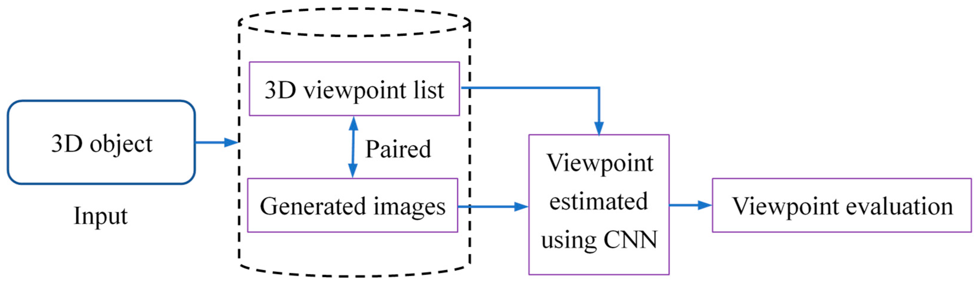
We propose an image-based viewpoint estimation method that demonstrates the complete process from creating a dataset to evaluating the results.
(2)
In the viewpoint position selection module, we integrate the initial viewpoint moving strategy into the spherical viewpoint uniform sampling based on analytical methods to enhance the effectiveness of spherical uniform random sampling.
(3)
A new dataset has been established and made available on the GitHub website. Based on the new dataset learning, we implemented image-based viewpoint estimation using a simple CNN. The viewpoint estimation results are evaluated based on the new accuracy calculation formula.
(4)
We use the viewpoint estimation method to analyze the chair display angles on a furniture website, illustrating the display angle preferences of merchants displaying items.
The remainder of the paper is organized as follows. Section 2 reviews related work. Section 3 describes the methods. Section 4 introduces the dataset and the implementation details. Section 5 concludes the paper by summarizing our study and future works.

2. Related Work

The existing literature on image-based viewpoint estimation can roughly be classified into three aspects: rule-based methods, machine learning-based methods, and evaluation.

2.1. Rule-Based Methods

The main idea of the rule-based methods for estimating viewpoints from object images is to analyze image features, such as statistical features and geometric features, and establish a mapping between these statistical features and the corresponding viewpoints. For example, in 1997, Takamatsu et al. [18] proposed a viewpoint estimation method based on moment features representing non-local image properties, including gravity center and breadth. This method demonstrated a lower computational cost and notable robustness to noise. It was found to be a connection between the 3D shape contour and the viewpoint [19]. To improve the viewpoint estimation accuracy, in 2018, Busto Pau et al. [2] proposed a domain adaptation approach that aligns the domain of the synthesized images with the domain of the actual images. In 2000, Sanchiz et al. [20] presented a method for estimating the viewpoint by identifying the minimum distance point to the set of step rays. In 2024, Sandro et al. used a Gaussian viewpoint estimator and an extended Kalman filter to predict the three-dimensional (3D) object’s position [21].
In summary, some typical features are listed in Table 1 as examples of these rule-based methods. Rule-based viewpoint estimation methods often perform feature analysis based on image content, so these methods are generally class-dependent. We did not adopt this viewpoint estimation method based on image feature analysis to make the construction method more versatile.

2.2. Machine Learning-Based Methods

In recent years, due to the widespread availability of online images and the establishment of labeled databases, machine learning-based methods have been widely explored. For example, in 2020, Mariotti et al. [22] proposed a semi-supervised viewpoint estimation method that can learn to infer viewpoint information from unlabeled image pairs, where two images differ by viewpoint change. Divon et al. [23] presented five key insights that should be taken into consideration when designing a CNN that solves the problem. Based on these insights, the paper proposes a network in which (i) the architecture jointly solves detection, classification, and viewpoint estimation; (ii) new types of data are added and trained on; And (iii) a novel loss function, which takes into account both the geometry of the problem and the new types of data, is proposed. In 2019, Shi et al. [14] proposed a viewpoint estimation method based on Convolutional Neural Networks (CNNs) for volume visualization. In 2021, Dutta et al. [24] proposed a self-supervised viewpoint estimation method that infers viewpoints from live camera images. This approach relies on a 3D model of the object and does not require manual data annotation or real images as input. In 2020, Joung et al. [25] developed a cylindrical convolutional network to estimate viewpoint.
A commendable viewpoint is that 3D models have the potential to generate a large number of images of high variation, which can be well exploited by deep CNNs with a high learning capacity [26]. Some work builds an image database with viewpoint labels before performing image-based viewpoint estimation on a given object. In 2015, Su H et al. [26] proposed a scalable and overfit-resistant image synthesis pipeline, together with a novel CNN specifically tailored for the viewpoint estimation task. In 2016, Wang Y et al. [27] built a CNN model to estimate object viewpoint from a single RGB image after generating a synthetic RGB image dataset with viewpoint annotations and extracting powerful features for the estimation. Several representative CNN models are listed in Table 2 as examples of these machine learning-based methods. Table 2 shows that these methods have established datasets, but unfortunately, these data have not been made public.
We have established a new dataset and made it public in this paper. In addition, unlike these references, we also provide a viewpoint sampling method to facilitate readers in establishing new datasets.

2.3. Evaluation

The quality evaluation of estimated viewpoints depends on labeled images and is primarily conducted through visual observation or quantitative indicator measurement. Regarding the accuracy of quantitative evaluation estimation, the method based on minimizing the empirical loss proposed in [22] is representative. Minimizing empirical loss means minimizing the total error between the estimated viewpoint direction and the actual viewpoint direction. In 2018, Meng M et al. [28] proposed a novel method of viewpoint quality evaluation (VQE), which utilizes texture distortion as an evaluation metric. The texture stretch and object fragment are taken as the main distortion factors. In 2010, Helin Dutagaci et al. [29] established a benchmark for the evaluation of best view selection algorithms. The benchmark consists of the preferred views of 68 3D models provided by 26 human subjects. In 2019, Zhang F et al. [30] presented a novel viewpoint evaluation method combining geometric and visual perception information. In 2022, Stewart E et al. [31] predicted the viewpoint similarity for rotated novel objects based on the projected position shifts of surface points as the object rotates.
Considering the outstanding performance of deep learning methods in image classification problems and their early exploration in viewpoint estimation problems, we adopt a new evaluation method combining a CNN and viewpoint estimation to achieve image-based viewpoint estimation.

3. Methods

Although our goal is to develop an image-based viewpoint estimation method, this issue also involves obtaining an image dataset with accurate viewpoint information and establishing a reasonable evaluation metric. Therefore, the proposed method consists of four modules: obtaining viewpoints, generating an image dataset with viewpoint annotations, estimating a viewpoint using a CNN, and evaluating the accuracy of the estimated viewpoint. The flow chart of the proposed method is shown in Figure 2.
In our flowchart, the first two modules, the obtaining viewpoints and the generating the image dataset with viewpoint annotations modules, are the same steps as the existing CNN-based methods listed in Table 2. The difference is that our method analyzes the selection of viewpoints, but these listed methods overlooked this point. The third module is the estimating viewpoint using a CNN without a rule-based module, given that the effectiveness of rule-based methods is trained in a class-dependent manner [26], with a comparison in Table 2. In the last module, viewpoint evaluation, an accuracy evaluation method with deviation angle tolerance is proposed.

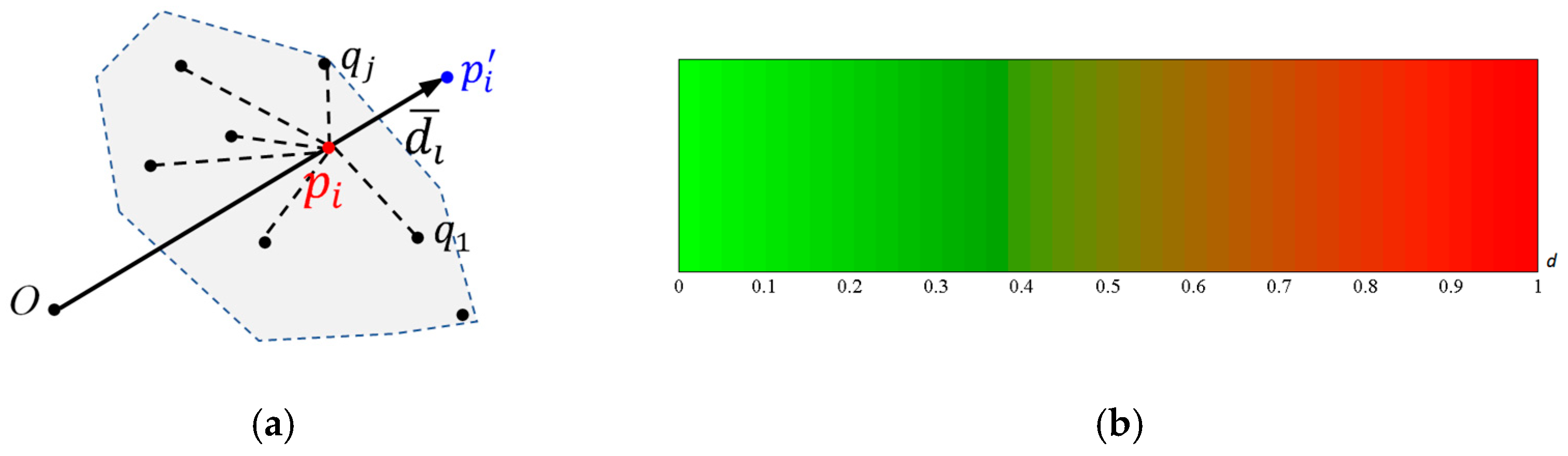
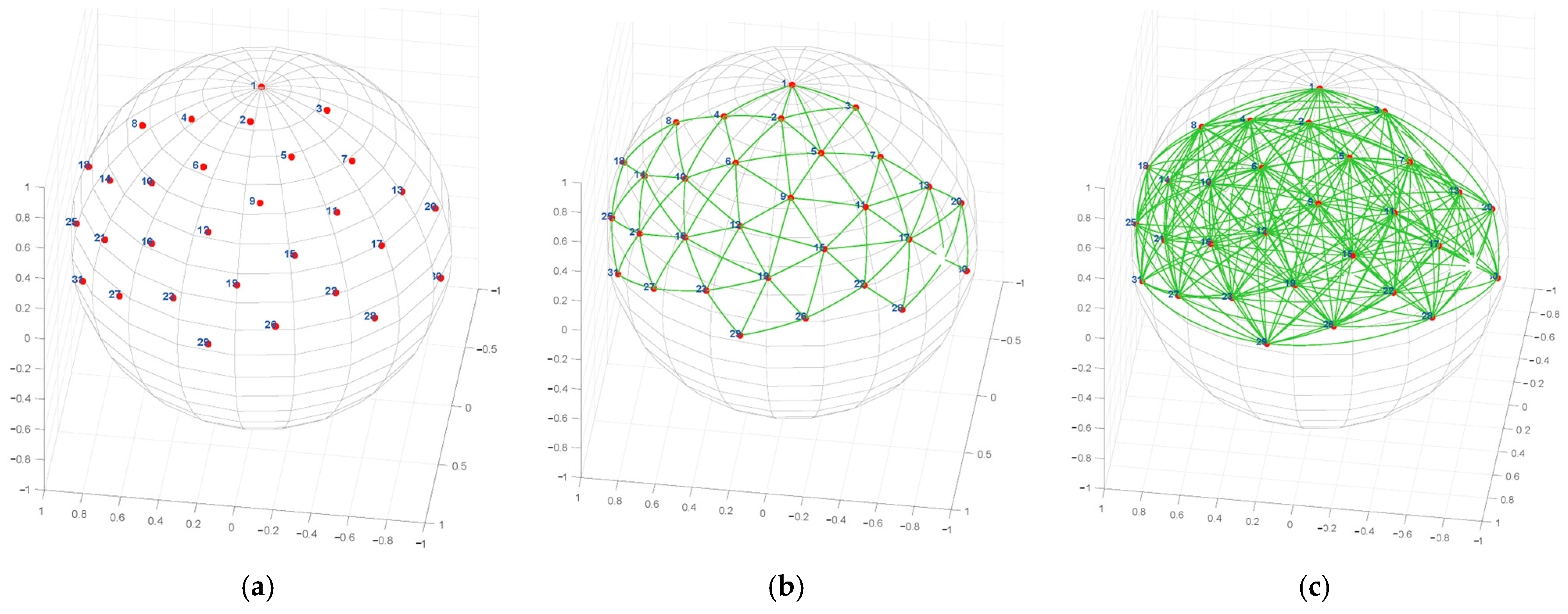
3.1. Uniform Sampling on a Unit Sphere

Similar to [16,32], a viewpoint for observing an object in three-dimensional (3D) space represents a viewpoint direction, which can be labeled as a point on the sphere surrounding the observed object. Therefore, generating random viewpoints on the sphere corresponds to the statistical problem of sampling on the sphere. The sphere is a curved space and the uniform sampling in this space is not an easy task. Traditionally, the implementation of uniform sampling on a sphere can be based on analytical formulas [33] or particle motion simulation. To improve the effect of sampling, we propose a new algorithm called the Fibonacci spherical uniform sampling algorithm based on repulsion and random optimization (FSUS-RR), combining the particle motion simulation with analytical formulas. The new sampling algorithm consists of two stages: generating sampling points through analytical methods, and moving sample points as particles. Through random experiments and verification, we chose the analytical method, the canonical Fibonacci lattice sampling method (CFLS) [33], to generate uniform sampling points on the unit sphere. Then, the initial sampling points are optimized by particle moving using two strategies: repulsion moving and random moving.
Letting d i n e i be the distance from viewpoint p i to its closest neighbor, the moving step m s t e p is directly proportional to the difference ( d m a x n e i d m i n n e i ), that is
m s t e p = τ ( d m a x n e i d m i n n e i ) / 2 ,
where
d m a x n e i = max j { d j n e i } ,   d m i n n e i = min j { d j n e i } .
Letting v j n e i be the unit vector from the closest neighbor of viewpoint p j to p j , the moving direction v s t e p is staggered, that is, the direction of repulsive force v i n e i and a random direction are alternately selected. The detail of our FSUS-RR is shown in Algorithm 1. This algorithm combines the sampling of analytical methods with a random movement strategy, achieving a balance between sampling efficiency and the uniform distribution effect; reasoning from this, the analytical method sampling has high efficiency in generating viewpoints, but the uniformity of sampling points is insufficient. The random movement method can improve the uniform distribution effect, but the sampling efficiency is low.
Algorithm 1: FSUS-RR
Input: N, //The number of sampling points,
    I i t e //The number of iterations
Output: V = { p i ( x i , y i , z i ) } //the coordinates of N points on the unit sphere
1: η = ( 1 + 5 ) / 2   //for steps 1 through 6, use the CFLS method [33]
2: for i   f r o m   0   t o   N 1
3:    ϑ = 2 π i / η
4:    φ = cos 1 ( 1 2 ( i + 0.5 ) / N )
5:    p i = ( x i , y i , z i ) = ( cos θ sin φ ,   sin θ sin φ ,   cos φ )
6: end
7: flag = 1;
8: for i   f r o m   1   t o   I i t e
9:    Build k d t r e e using all sampling points { p i ( x i , y i , z i ) }
10:   Calculating m s t e p using Equation (1)
11:  for j from 1 to N
12:    if flag == 1, then
13:     v s t e p = v j n e i
14:    else
15:     v s t e p is a random unit vector
16:    end
17:    p j = p j + m s t e p × v s t e p //Update the position of p j
18:    flag = 1-flag
19:    p j = p j / p j  //In terms of vector units
20:   end
21: end
22: Output the sampling points V = { p i ( x i , y i , z i ) }
To verify the effectiveness of our method, we conducted comparative experiments. Several representative methods include the CFLS [33], Continuous Stochastic Dynamics (CSDyn) [34], Inverse Transform sampling (https://github.com/benroberts999/inverseTransformSample, access date: 10 March 2025) (InveT), analytically exact spiral scheme (Spiral) [35], sampling of concentric spherical shells in k-space with the new strategy (Kspace) [36], the traditional Spherical Coordinate Sampling using Azimuthal rotation and the Polar rotation (SCS-AP), and ours. The spherical sampling results of these methods are shown in the first row of Figure 3.
The differences between these results are easily noticeable when the number of points is small. When the number of points is relatively large, the difference is not obvious. We design a method to visualize the uniform distribution effect here. For any sampling point p m , the average distance of p m to its k nearest neighbors q j ( j = 1 , 2 , , k ) can be calculated (Figure 4a) as
d ¯ m = 1 k j = 1 k p m q j 2 .
where p m q j 2 is the 2-norm distance between point p m and its neighbor point q j .
Then, we let p m move to a new position p i using the bellow formula.
p m = p m + d ¯ m × O p m o .
where O p m o is the unit vector parallel to O p m . In addition, to enhance the visualization effect, we also design a coloring scheme (Figure 4b) for the moved sampling points. The sampling results are visualized in Figure 5. If the uniform sampling of the sphere is uniform, then the colored sphere is a perfectly spherical shape and the coloring is also evenly distributed. The best result is that the colors are the same within the sphere. Based on these two visual indicators, our method demonstrates the best performance among these seven methods.
In addition to comparing visual effects, we also quantitatively analyze and compare the spherical sampling results of various methods. Quantitative analysis is mainly conducted on the average distance between neighbors, calculated by Formula (3). An assumption is that, in an ideal uniform sampling, the average distance d ¯ m ( m = 1 , 2 , , N ) between the neighbors of each point should be the same. Therefore, we calculate the minimum (minAveD), maximum (maxAveD), and standard deviation (stdAveD) of the average distance { d ¯ m , m = 1 , 2 , , N } between the nearest neighbors of all points, and perform a Kolmogorov–Smirnov (KS) test for uniform distribution and normal distribution. N is the number of sampling points, and we test three sampling densities, namely N = 25, 250, and 900, corresponding to the cases of a few, a medium number, and many points, respectively. The quantitative index calculation results of the sampling points obtained by seven methods are shown in Table 3, Table 4 and Table 5.
According to these quantitative index calculation results of the sampling points, our method generally demonstrates the best performance according to the four evaluation metrics: maxAveD, Range, stdAveD, and NrmHks. The proposed method is similar to other methods for the remaining five indicators. For example, our minimum distance is relatively large, ranking second among all methods, which is also quite good. Because we use analytical methods to calculate the initial viewpoint position and then use random movement to improve uniformity, the calculation time among these five indicators is more prolonged than using analytical methods alone, but it is more efficient than using the random movement method alone.

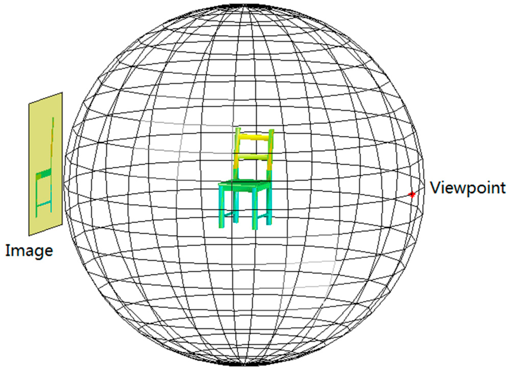
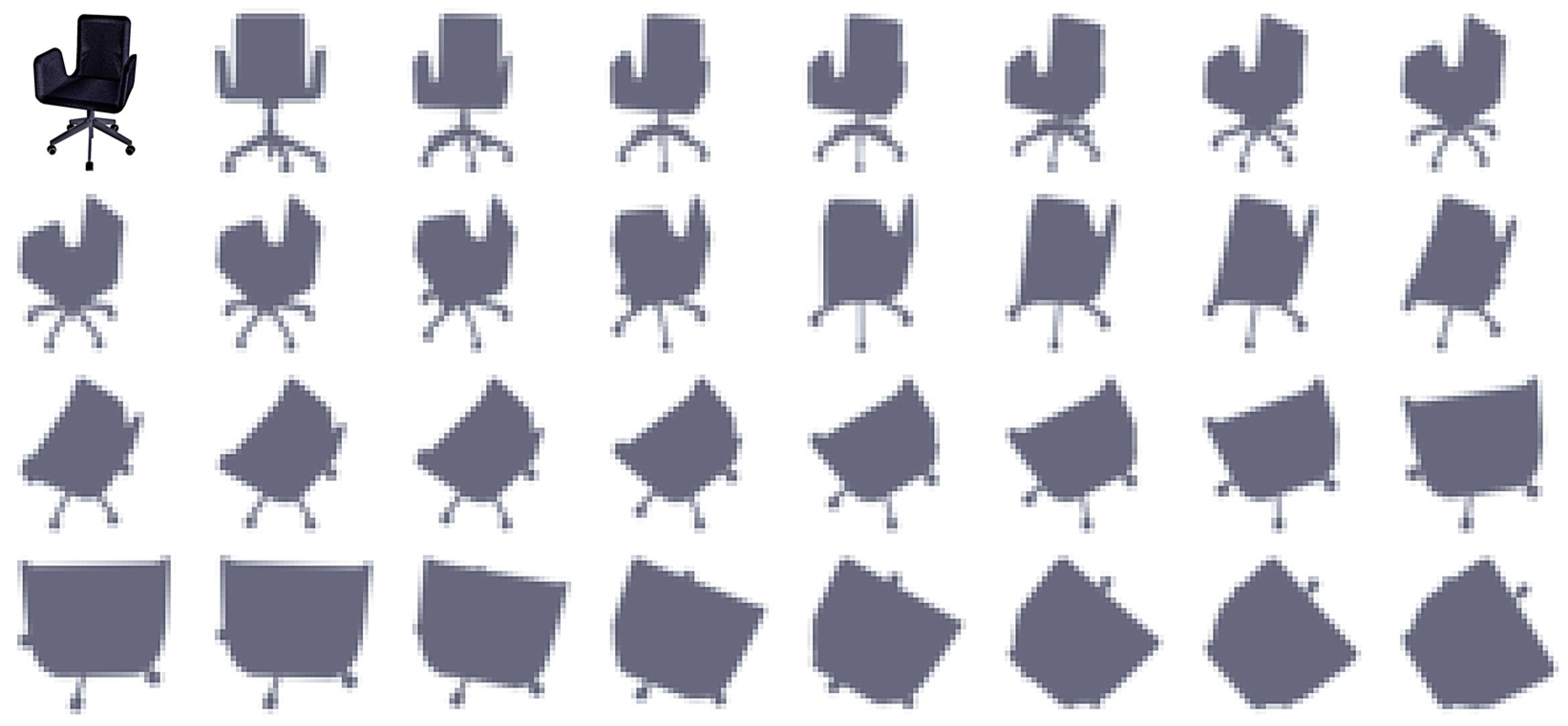
3.2. Image Generated According to Viewpoints

After selecting viewpoints using Algorithm 1, the dataset for image viewpoint estimation can be constructed. We utilize 3D models to perform parallel projection based on the specified viewpoint directions, thereby generating 2D projection images. This process is illustrated in Figure 6.
Due to the different sizes of the models, it is necessary to standardize them into a fixed size. Let N v be the number of vertices of the 3D object model, and V i x i , y i , z i ( i = 1 , 2 , , N v ) the ith vertex of the model. Then, this model can be standardized using the following formula:
Q i n e w = γ o R o ( V i O c n t ) ,   i = 1 , 2 , , N v .
where γ o is a scale factor, and we use γ o = 0.45 as the default value; R o is the diameter of the object; and O c n t is the geometric center of the object. That is,
O c n t = 1 N v i = 1 N v V i
After standardizing the model using Equation (5), it can be completely enclosed within the unit sphere.
With the standardized model and the viewpoints obtained according to Section 3.1, projection images with viewpoint labels can be obtained through parallel projection based on the viewpoint direction. The mathematical formulas for parallel projection based on the direction of the viewpoint p v i e w ( p v i e w = 1 ) can be formulated as
Q n = Q o ( p v i e w · O Q o ) p v i e w .
where Q o is any vertex of the 3D object of which the center has been translated to the origin, and Q n is the projection point of Q o on the projected image. The algorithm for generating images according to specified viewpoints (Algorithm 2) is described as follows. In the process of generating this image with a viewpoint label, Algorithm 1 is the first step in Algorithm 2.
Algorithm 2: Generating images according to specified viewpoints
Input: ϑ L , ϑ U , //rang ϑ L ϑ ϑ U ,
    φ L , φ U , //rang φ L φ φ U ,
    d v p , //The minimum distance between neighboring viewpoints
    I r , I c .//The size of the output image
Output: Ω = { I i , ϑ i , φ i } //images with labeled viewpoints
1: Generate viewpoints using Algorithm 1;
2: Remove viewpoints that are not within the specified ranges;
3: Remove neighboring viewpoints with distances less than d v p ;
4: Generate a projection image for each viewpoint using Equation (7);
5: Construct the AABB (Axially Aligned Bounding Box) of the object projection image, and cut off the external redundant margins which are out of the AABB;
6: Enlarge or reduce the image to the specified size (e.g., 32 × 32 );
7: Output the   images   Ω = { I i , ϑ i , φ i } to a folder.
In the labeled image dataset, the viewpoints we have chosen are in front of the upper hemisphere, considering that the viewpoint is often higher than the horizontal line of sight in most applications, such as autonomous driving or furniture exhibitions.

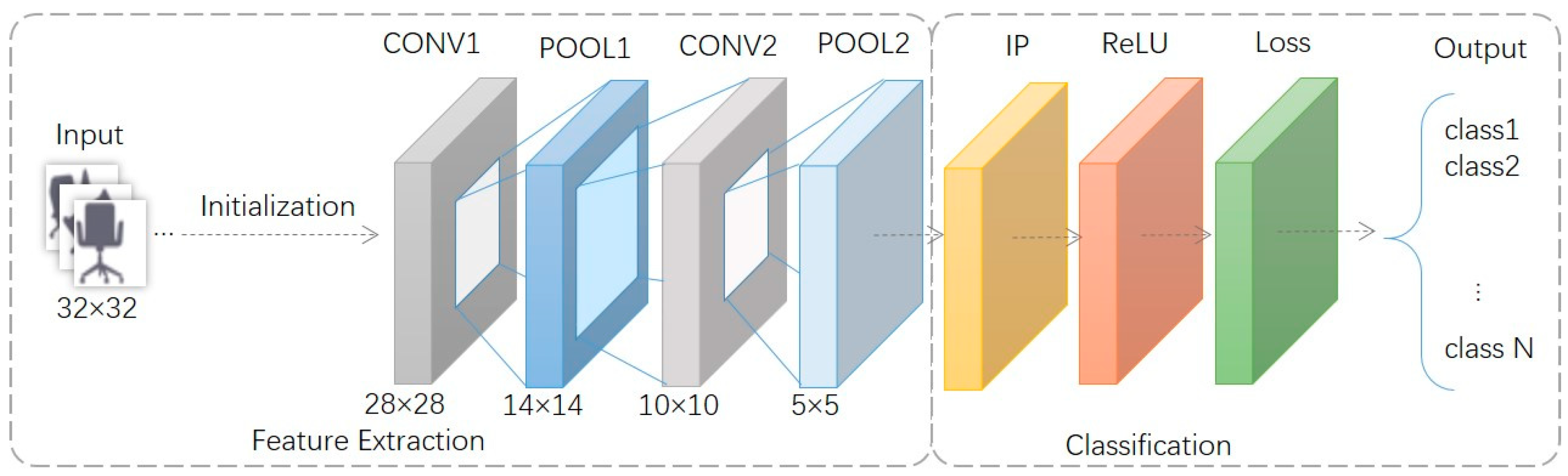
3.3. Viewpoint Estimated Using CNN

Deep learning-based image classification has achieved remarkable success since 2006. Because of the difference between viewpoint estimation and image classification, we utilize a deep learning model for image classification with viewpoint labels after developing a new soft accuracy function. The accuracy function allows for the perspective estimation bias, which is defined as follows.
A c c = 1 N m = 1 N δ m ,
where N is the number of images, and
δ m = O P m e s t · O P m g t , i f   O P m e s t · O P m g t c o s ( δ 0 ) 0 , o t h e r w i s e .
In Equation (9), m is the m t h image, and δ 0 the threshold which is the maximum tolerable viewpoint deviation angle. Since our study utilizes a unit vector to represent a viewpoint direction, the inner product O P m e s t · O P m g t of the vectors O P m e s t and O P m g t directly corresponds to the cosine value of the angle between these two vectors.
According to the algorithm in Section 3.2, we have constructed an image dataset with viewpoint position labels. These images are classified according to the viewpoint positions. Using Equation (9), the loss function can be rewritten. After completing the dataset construction and loss function design, a simple CNN framework [37] is established to achieve image-based viewpoint estimation. This CNN framework consists of seven layers, and its architecture and parameters are illustrated in Figure 7.

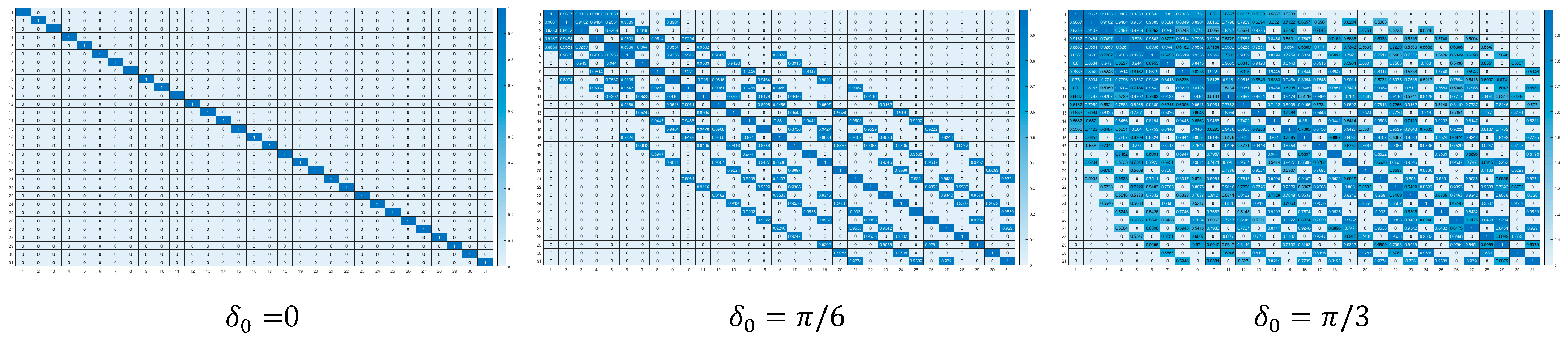
3.4. Accuracy Evaluation of Estimated Viewpoint

During the model testing phase, or when comparing image-based viewpoint estimation methods, the accuracy of image-based viewpoint estimation is also evaluated using Equations (8) and (9). The value of the parameter δ 0 can be specified by the user based on the number of viewpoints and error tolerance. For example, δ 0 = π / 6 .

4. Experiment

The experiment aims to evaluate the proposed method (Figure 2) and assess its effectiveness through three aspects: viewpoint image dataset construction, parameter sensitivity analysis, and image-based viewpoint estimation performance evaluation. Our algorithms are implemented in MATLAB (2018). Each run is executed on a single thread on a personal desktop computer, and the computer configuration is Intel (R) Core (TM) i9-9700 CPU @ 3.00 GHz processor and 16 GB RAM per run. The runtime for each parameter setting is measured as the average execution time (in seconds) of five repeated experiments.

4.1. Dataset

Considering furniture sale cases, furniture is displayed to customers through images captured from optimal viewpoints. Our experiment aims to estimate the viewpoint based on these furniture images, primarily featuring chairs, stools, and sofas.
First, we downloaded an open dataset [38]. This dataset consists of over a hundred 3D furniture models. Among them, 29 objects, including chairs, stools, and sofas, were selected for our viewpoint screenshot experiment.
Then, we applied Algorithm 1 to generate viewpoints on the unit sphere. In this experiment, we selected only 31 viewpoints in front of the object in the upper hemisphere, as illustrated in Figure 8a.
Finally, we utilized Algorithm 2 to generate images based on these specified viewpoints. The dataset used in our experiments consists of 31 viewpoint classes, each with 29 images. Therefore, the generated dataset consists of 899 images divided into 31 categories, with 29 images per category. Figure 9 presents 31 images of the same object projected from 31 different viewpoints.

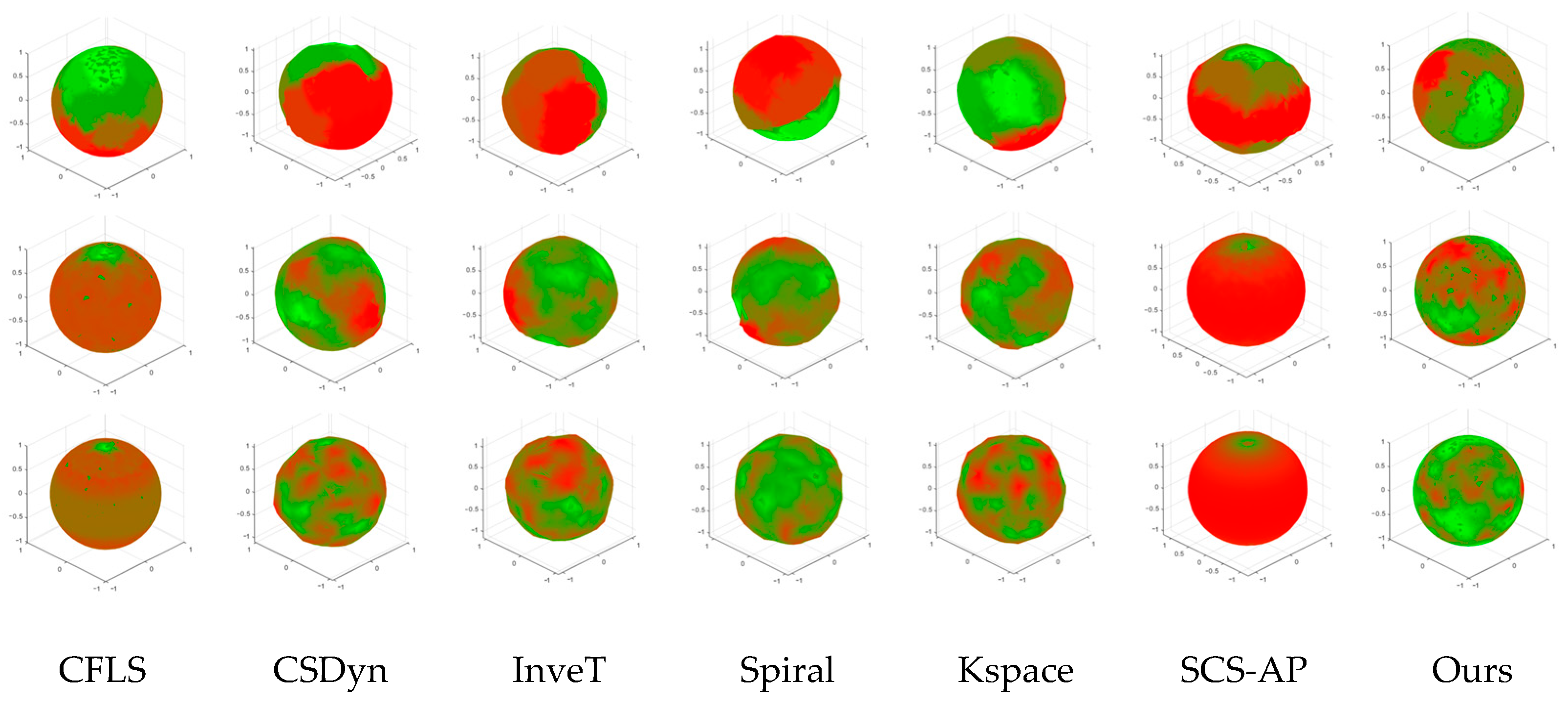
4.2. Parameter Analysis and Comparisons

In Algorithm 1, the parameters are defined based on a random distance and do not require user specification. Parameter I i t e , the number of iterations, according to our experiment, has a minor impact on the distribution when the number of points is relatively small, e.g., less than 30. If N > 30 , we set I i t e = 2500 times as the default value.
In Section 3.3 and Section 3.4, parameter δ 0 , the maximum tolerable viewpoint deviation angle, significantly affects the accuracy value. If δ 0 = 0 , an estimated viewpoint is considered correct only if it perfectly coincides with the ground truth viewpoint; otherwise, it is considered incorrect. In this case, the formula for calculating the classification accuracy follows the standard accuracy formula used in image classification. The accuracy calculation method for viewpoint estimation proposed in this study is an extension of the traditional accuracy calculation method for image classification. The smaller the value, the stricter the accuracy criterion, allowing for less error tolerance.
We experimented to demonstrate the effectiveness of using our method for viewpoint estimation. Using δ 0 = 0 , π / 6 , π / 3 , the nearest neighbor relationships of the 31 viewpoints are represented by a distance matrix, as shown in Figure 10.

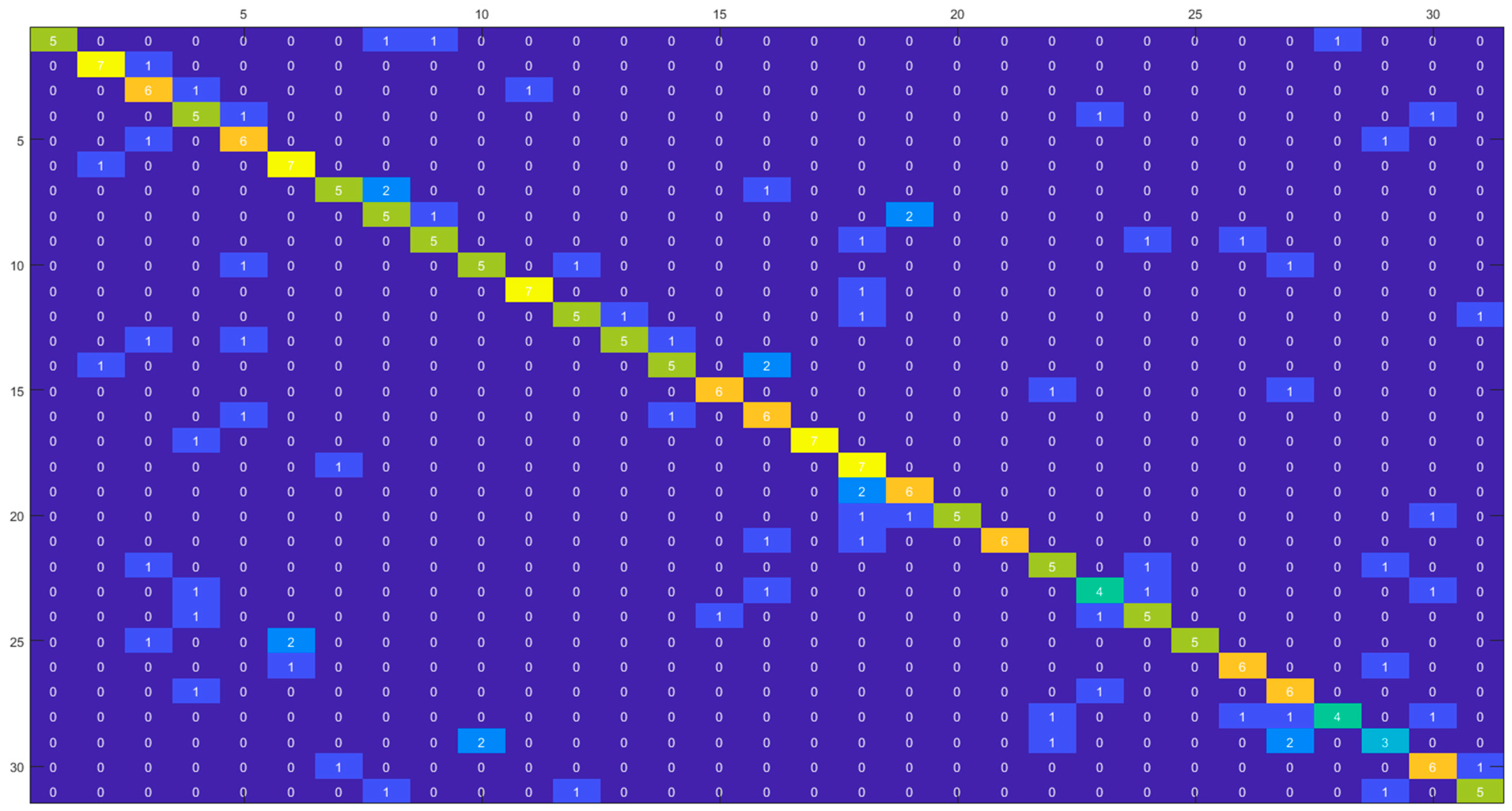
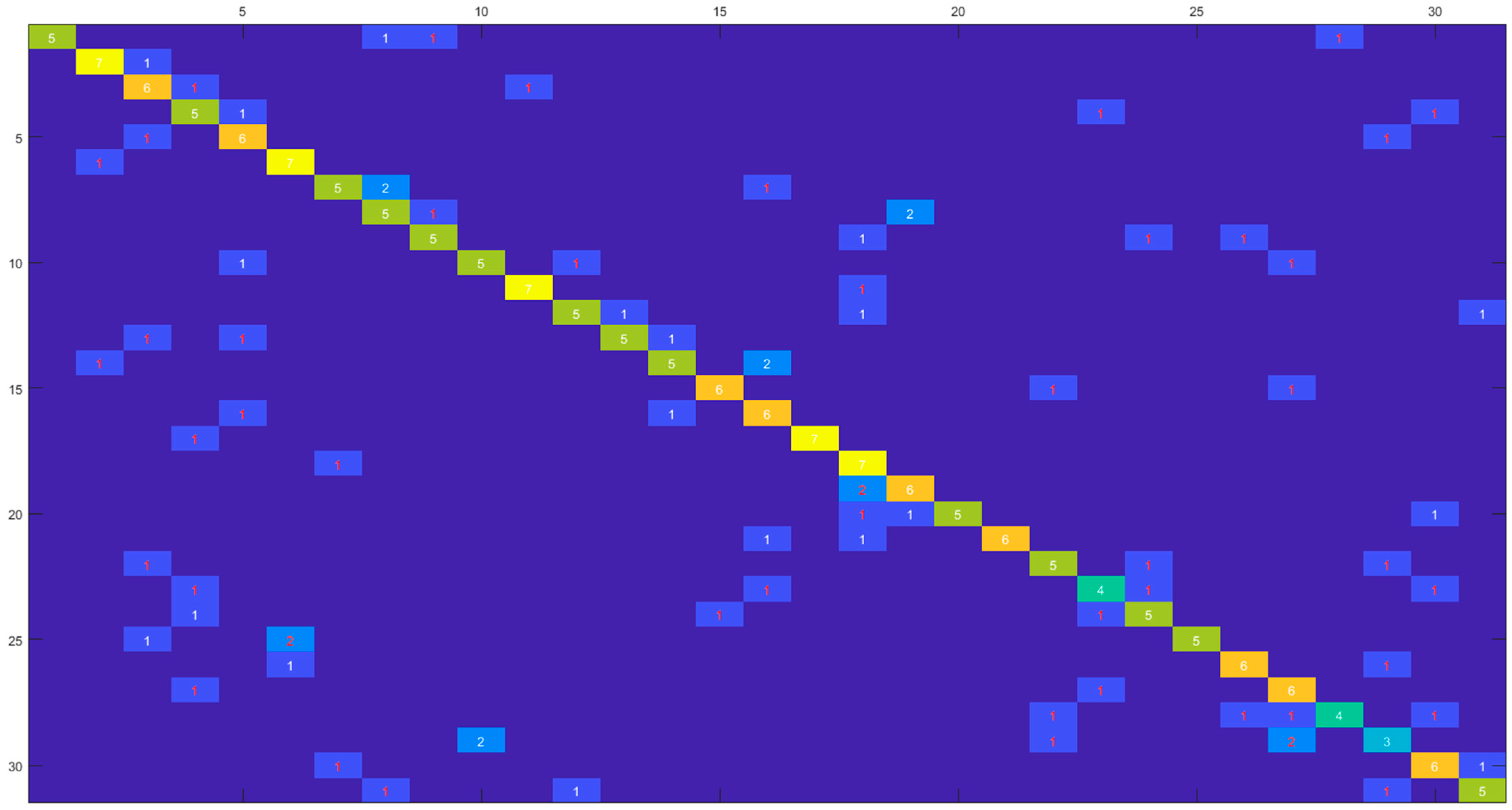
4.3. Viewpoint Estimation Results

From the generated dataset, we randomly select 75 % × N images for training, where x rounds number x to the lower integer. Since each class consists of 29 images, there are 21 images in each class in the training set, and the remaining eight images are used for testing. The maximum number of iterations is set to 20,000, with other parameters set to their default values. The training process takes 10,719.46 s, and the training accuracy is 100% due to the small training set. The confusion matrix of the test set is shown as a heat map in Figure 11. By summing the diagonal elements and taking the total number of images, the classification accuracy can be calculated to be 0.6855, corresponding to δ 0 = 0 .
If the viewpoint evaluation method with the angle deviation metric proposed in this article is adopted, with a tolerance angle of 30 degrees ( δ 0 = π / 6 ), as shown in Figure 8b, the accuracy of the viewpoint estimation is 0.8105. The number of images with deviation angles within π / 6 is marked as a red number in the confusion matrix in Figure 12.
Similarly, if we increase the deviation angle to 60 degrees ( δ 0 = π / 3 ), as shown in Figure 8c, the accuracy of the viewpoint estimation increases to 0.8911, improved by approximately 9.94% compared to δ 0 = π / 6 . The number of images with deviation angles within π / 3 is also marked as a red number in the confusion matrix in Figure 13.

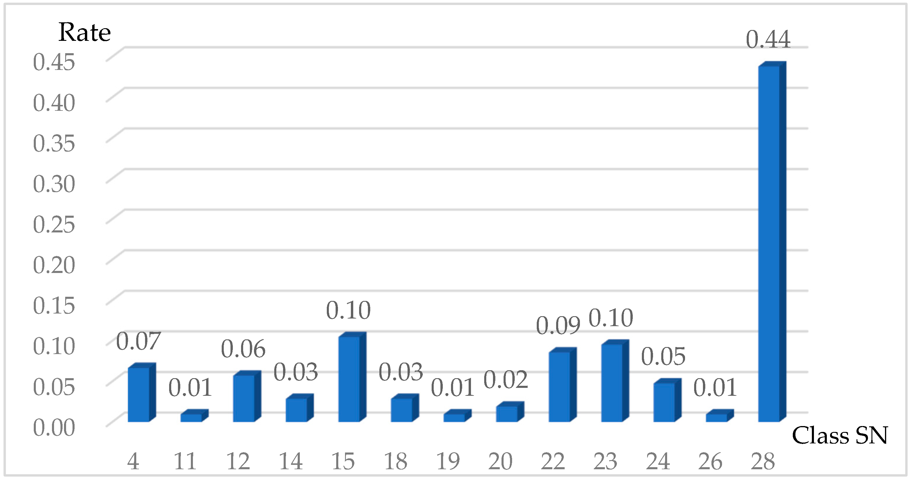
4.4. Application to Display Image Analysis

One application of viewpoint estimation is the analysis of the display angle of objects. Among various object displays, the chair display is the most closely related to our training set. Therefore, we use it as an example to illustrate the application of our method. We downloaded chair images from the Nitori company website (https://www.nitori-net.jp/ec/cat/Chair/, access date: 12 February 2025). We randomly chose chair products across different categories and used the first image of the product profile page. A total of 105 chair images were analyzed using viewpoint estimation with our method. The estimated viewpoints were then visualized using a frequency distribution histogram, as shown in Figure 14. From the figure, we observe that only 13 viewpoints are adopted by the company, and 44% of the images were captured from the same viewpoint, the 28th viewpoint. This perspective corresponds to a right-side, slightly upward-angled shot of the chair. This application illustrates that we can infer the preference of the website display angles for items using our proposed viewpoint estimation method.

5. Conclusions

In this paper, we propose an image-based method for viewpoint estimation; verify that using a sampling point movement strategy to improve the uniform distribution of initial spherical viewpoints generated by analytical methods reduces the average distance of the maximum nearest neighbors; generate a small image dataset with viewpoint markers; and develop a calculation method for the accuracy of viewpoint estimation that integrates deviation angles. The viewpoint estimation experiments show that the accuracy of CNN-based estimation can be improved from 68.55% to 81.05% when the viewpoint angle deviation is π / 6 ; the proposed viewpoint estimation method can be used for analyzing the display angle of chairs on furniture websites.
The main limitations of our method are that the CNN model in the algorithm framework is simple and lacks a comprehensive selection of various viewpoint estimation models, and the newly established dataset is too small. Although comprehensive selection is not the focus of this paper, it is a worthwhile direction for future research. If a comprehensive model selection is conducted and a more suitable machine learning model is found, the accuracy of viewpoint estimation can be improved. The scale of image datasets with viewpoint annotations provided in existing papers, including this paper, is still too small, so it is worth looking forward to generating large datasets and providing them to the public for use.

Author Contributions

Conceptualization, M.Y. and H.L.; methodology, M.Y. and H.L.; software, H.L.; validation, M.Y. and H.L.; formal analysis, H.L.; investigation, M.Y. and H.L.; resources, M.Y. and H.L.; data curation, M.Y. and H.L.; writing—original draft preparation, M.Y. and H.L.; writing—review and editing, M.Y. and H.L.; visualization, M.Y.; supervision, H.L.; project administration, H.L. All authors have read and agreed to the published version of the manuscript.

Funding

This research received no external funding.

Data Availability Statement

The newly created data and code are available at https://github.com/Hongjun2025/ImageViewpoint, access date: 12 March 2025.

Acknowledgments

The author thanks the anonymous referees for their valuable suggestions.

Conflicts of Interest

The authors declare no conflicts of interest. The funders had no role in the design of the study; in the collection, analyses, or interpretation of data; in the writing of the manuscript; or in the decision to publish the results.

References

  1. Zhang, Y.; Fei, G.; Yang, G. 3D Viewpoint Estimation Based on Aesthetics. IEEE Access 2020, 8, 108602–108621. [Google Scholar] [CrossRef]
  2. Busto, P.P.; Gall, J. Viewpoint Refinement and Estimation with Adapted Synthetic Data. Comput. Vis. Image Underst. 2018, 169, 75–89. [Google Scholar] [CrossRef]
  3. Xiao, Y.; Lepetit, V.; Marlet, R. Few-shot Object Detection and Viewpoint Estimation for Objects in the Wild. IEEE Trans. Pattern Anal. Mach. Intell. 2022, 45, 3090–3106. [Google Scholar] [CrossRef] [PubMed]
  4. Kucerova, J.; Varhanikova, I.; Cernekova, Z. Best View Methods Suitability for Different Types of Objects. In Proceedings of the Spring Conference on Computer Graphics, Smolenice, Slovakia, 2–4 May 2012; pp. 55–61. [Google Scholar] [CrossRef]
  5. Sweet, G.; Ware, C. View Direction, Surface Orientation and Texture Orientation for Perception of Surface Shape. In Proceedings of the Graphics Interface Conference, London, ON, Canada, 17–19 May 2004; DBLP: London, ON, Canada, 2004. [Google Scholar] [CrossRef]
  6. Li, T.; Yang, L.; Wang, M.; Fan, Y.; Zhang, F.; Guo, S.; Chang, J.; Zhang, J.J. Visual Saliency-Based Bas-Relief Generation with Symmetry Composition Rule. Comput. Animat. Virtual Worlds 2018, 29, e1815. [Google Scholar] [CrossRef]
  7. Zhou, W.; Jia, J. Training Deep Convolutional Neural Networks to Acquire the Best View of a 3D Shape. Multimedia Tools Appl. 2020, 79, 581–601. [Google Scholar] [CrossRef]
  8. Liu, H.; Zhang, L.; Huang, H. Web-image driven best views of 3D shapes. Vis. Comput. 2012, 28, 279–287. [Google Scholar] [CrossRef]
  9. Collander, C.; Beksi, W.J.; Huber, M. Learning the Next Best View for 3D Point Clouds via Topological Features. arXiv 2021. [Google Scholar] [CrossRef]
  10. Ghezelghieh, M.F.; Kasturi, R.; Sarkar, S. Learning Camera Viewpoint Using CNN to Improve 3D Body Pose Estimation. In Proceedings of the 2016 Fourth International Conference on 3D Vision (3DV), Stanford, CA, USA, 25–28 October 2016; IEEE: Stanford, CA, USA, 2016. [Google Scholar] [CrossRef]
  11. He, J.; Zhou, W.; Wang, L.; Zhang, H.; Guo, Y. Viewpoint Selection for Taking a Good Photograph of Architecture. Eurographics Assoc. 2016, 39–44. [Google Scholar] [CrossRef]
  12. Abdulwahab, S.; Rashwan, H.A.; García, M.Á.; Jabreel, M.; Chambon, S.; Puig, D. Adversarial Learning for Depth and Viewpoint Estimation from a Single Image. IEEE Trans. Circuits Syst. Video Technol. 2020, 30, 2947–2958. [Google Scholar] [CrossRef]
  13. Sun, X.; Lian, Z. EasyMesh: An Efficient Method to Reconstruct 3D Mesh from a Single Image. Comput. Aided Geom. Des. 2020, 80, 101862. [Google Scholar] [CrossRef]
  14. Shi, N.; Tao, Y. CNNs-Based Viewpoint Estimation for Volume Visualization. ACM Trans. Intell. Syst. Technol. 2019, 10, 27. [Google Scholar] [CrossRef]
  15. Mustikovela, S.K.; Jampani, V.; Mello, S.D.; Liu, S.; Iqbal, U.; Rother, C.; Kautz, J. Self-Supervised Viewpoint Learning from Image Collections. In Proceedings of the Computer Vision and Pattern Recognition, Seattle, WA, USA, 16–18 June 2020; IEEE: Seattle, WA, USA, 2020. [Google Scholar] [CrossRef]
  16. Gu, C.; Lu, C.; Gu, C.; Guan, X. Viewpoint Estimation Using Triplet Loss with a Novel Viewpoint-Based Input Selection Strategy. J. Phys. Conf. Ser. 2019, 1207, 012009. [Google Scholar] [CrossRef]
  17. Kim, Y.; Hyunwoo, H.; Kim, Y.; Surh, J.; Ha, H.; Oh, T.H. MeTTA: Single-View to 3D Textured Mesh Reconstruction with Test-Time Adaptation. In Proceedings of the 35th British Machine Vision Conference 2024, {BMVC} 2024, Glasgow, UK, 25–28 November 2024; poster. Available online: https://bmva-archive.org.uk/bmvc/2024/papers/Paper_18/paper.pdf (accessed on 12 February 2025).
  18. Takamatsu, R.; Takada, Y.; Sato, M. Viewpoint Estimation Based on Moment Feature. J. Inst. Image Inf. Telev. Eng. 1997, 51, 1262–1269. [Google Scholar] [CrossRef]
  19. Zhao, L.; Liang, S.; Jia, J.; Wei, Y. Learning Best Views of 3D Shapes from Sketch Contour. Vis. Comput. 2015, 31, 765–774. [Google Scholar] [CrossRef]
  20. Sanchiz, J.M.; Fisher, R.B. Viewpoint Estimation in Three-Dimensional Images Taken with Perspective Range Sensors. IEEE Trans. Pattern Anal. Mach. Intell. 2000, 22, 1324–1329. [Google Scholar] [CrossRef]
  21. Sandro, C.; António, P.; Filipe, N.; Jorge, D. BVE + EKF: A Viewpoint Estimator for the Estimation of the Object’s Position in the 3D Task Space using Extended Kalman Filters. In Proceedings of the 21st International Conference on Informatics in Control, Automation and Robotics—Volume 2: ICINCO, Porto, Portugal, 18–20 November 2024; SciTePress: Porto, Portugal, 2024; pp. 157–165. [Google Scholar] [CrossRef]
  22. Mariotti, O.; Bilen, H. Semi-Supervised Viewpoint Estimation with Geometry-Aware Conditional Generation. In Computer Vision—ECCV 2020 Workshops; Lecture Notes in Computer Science; Springer: Cham, Switzerland, 2020; Volume 12536. [Google Scholar] [CrossRef]
  23. Divon, G.; Tal, A. Viewpoint Estimation—Insights and Model. In Computer Vision—ECCV 2018. ECCV 2018; Lecture Notes in Computer Science; Ferrari, V., Hebert, M., Sminchisescu, C., Weiss, Y., Eds.; Springer: Cham, Switzerland, 2018; Volume 11218, pp. 265–281. [Google Scholar] [CrossRef]
  24. Dutta, S.; Rauhut, M.; Hagen, H.; Gospodnetić, P. Automatic Viewpoint Estimation for Inspection Planning Purposes. In Proceedings of the 2021 International Conference on Image Processing and Computer Vision, Anchorage, AK, USA, 19–22 September 2021; Springer: Cham, Switzerland, 2021. [Google Scholar] [CrossRef]
  25. Joung, S.; Kim, S.; Kim, H.; Kim, M.; Kim, I.-J.; Cho, J.; Sohn, K. Cylindrical Convolutional Networks for Joint Object Detection and Viewpoint Estimation. In Proceedings of the IEEE/CVF Conference on Computer Vision and Pattern Recognition (CVPR), Seattle, WA, USA, 16–18 June 2020. [Google Scholar] [CrossRef]
  26. Su, H.; Qi, C.R.; Li, Y.; Guibas, L.J. Render for CNN: Viewpoint Estimation in Images Using CNNs Trained with Rendered 3D Model Views. In Proceedings of the 2015 IEEE International Conference on Computer Vision (ICCV), Santiago, Chile, 7–13 December 2015; IEEE: Santiago, Chile, 2015. [Google Scholar] [CrossRef]
  27. Wang, Y.; Li, S.; Jia, M.; Liang, W. Viewpoint Estimation for Objects with Convolutional Neural Network Trained on Synthetic Images. In Proceedings of the 2016 International Conference on Artificial Intelligence and Pattern Recognition, Lodz, Poland, 19–21 September 2016; Springer: Cham, Switzerland, 2016. [Google Scholar] [CrossRef]
  28. Meng, M.; Zhou, Y.; Tan, C.; Zhou, Z. Viewpoint Quality Evaluation for Augmented Virtual Environment. In Proceedings of the Pacific-Rim Conference on Multimedia, Hefei, China, 21–22 September 2018. [Google Scholar]
  29. Dutagaci, H.; Cheung, C.P.; Godil, A. A Benchmark for Best View Selection of 3D Objects. In Proceedings of the 3DOR’10 Conference, Firenze, Italy, 25 October 2010. [Google Scholar]
  30. Zhang, F.; Li, M.; Wang, X.; Wang, M.; Tang, Q. 3D Scene Viewpoint Selection Based on Chaos-Particle Swarm Optimization. In Proceedings of the Chinese CHI 2019 Conference, Xiamen, China, 27–30 June 2019. [Google Scholar] [CrossRef]
  31. Stewart, E.E.M.; Hartmann, F.; Fleming, R. Viewpoint Similarity of 3D Objects Predicted by Image-Plane Position Shifts. J. Vis. 2022, 22, 3886. [Google Scholar] [CrossRef]
  32. Zhang, L.-J.; Gu, C.-C.; Wu, K.-J.; Huang, Y.; Guan, X.-P. Model-Based Active Viewpoint Transfer for Purposive Perception. In Proceedings of the 2017 13th IEEE Conference on Automation Science and Engineering (CASE), Xi’an, China, 20–23 August 2017; pp. 1085–1089. [Google Scholar] [CrossRef]
  33. Roberts, M. How to Evenly Distribute Points on a Sphere More Effectively than the Canonical Fibonacci Lattice. Extreme Learning Blog. 29 January 2024. Available online: https://extremelearning.com.au/how-to-evenly-distribute-points-on-a-sphere-more-effectively-than-the-canonical-fibonacci-lattice/ (accessed on 24 May 2024).
  34. Leimkuhler, B.; Stoltz, G. Sampling Techniques for Computational Statistical Physics. In Encyclopedia of Applied and Computational Mathematics; Springer: Berlin/Heidelberg, Germany, 2015; pp. 1287–1292. [Google Scholar] [CrossRef]
  35. Koay, C.G. Analytically Exact Spiral Scheme for Generating Uniformly Distributed Points on the Unit Sphere. J. Comput. Sci. 2011, 2, 88–91. [Google Scholar] [CrossRef] [PubMed]
  36. Wong, S.T.S.; Roos, M.S. A Strategy for Sampling on a Sphere Applied to 3D Selective RF Pulse Design. Magn. Reson. Med. 1994, 32, 778–784. [Google Scholar] [CrossRef] [PubMed]
  37. LeCun, Y.; Bottou, L. Gradient-Based Learning Applied to Document Recognition. Proc. IEEE 1998, 86, 2278–2324. [Google Scholar] [CrossRef]
  38. Lim, J.J.; Pirsiavash, H.; Torralba, A. Parsing IKEA Objects: Fine Pose Estimation. In Proceedings of the 2013 IEEE International Conference on Computer Vision (ICCV), Sydney, Australia, 1–8 December 2014; IEEE: Sydney, Australia, 2014. [Google Scholar] [CrossRef]
Figure 1. Three chairs displayed from different viewpoints. (a) A chair displayed from the upper right viewpoint; (b) The chair displayed from the upper left viewpoint; (c) Another chair displayed from the upper right viewpoint.
Algorithms 18 00224 g001
Figure 2. The flowchart of the proposed method.
Algorithms 18 00224 g002
Figure 3. The spherical uniform sampling results of seven methods. From top to bottom, the number of sampling points are 25, 250, and 900. (Please zoom in for a clear view.)
Algorithms 18 00224 g003
Figure 4. Schematic diagram of visualization scheme of the nearest neighbor average distance. (a) Moving direction; and (b) color scheme.
Algorithms 18 00224 g004
Figure 5. The visualization of the average distance of k nearest neighbors of each sampling point, generated using seven methods. The color represents the nearest neighbor average distance using the color scheme of Figure 4b.
Algorithms 18 00224 g005
Figure 6. A schematic diagram of generating a projection image through parallel projection according to the specified viewpoint position.
Algorithms 18 00224 g006
Figure 7. CNN model architecture for image-based viewpoint estimation.
Algorithms 18 00224 g007
Figure 8. Thirty-one viewpoints in front of the object in the upper hemisphere are used to construct viewpoint-related projection images, and a neighbor topology link graph with three neighbor angles. The colors of lines and fonts are only used for differentiation and have no other meaning. The number next to the vertex is the sequence number of the sampling viewpoint. (a) The neighbor ship is built according to δ 0 = 0 ; (b) The neighbor ship is built according to δ 0 = π / 6 ; (c) The neighbor ship is built according to δ 0 = π / 3 .
Algorithms 18 00224 g008
Figure 9. Thirty-one images are projected from the same chair along 31 different viewpoints. The top-left sub-image is a 3D model, while the remaining images are 31 projection images from different viewpoints.
Algorithms 18 00224 g009
Figure 10. The nearest neighbor relationships of 31 viewpoints when δ 0 = 0 , π / 6 , π / 3 .
Algorithms 18 00224 g010
Figure 11. Using the traditional method to calculate the confusion matrix of the classification results of the test set. The colors are only used for differentiation and have no other meaning.
Algorithms 18 00224 g011
Figure 12. The confusion matrix of the classification results of the test set when δ 0 = π / 6 .
Algorithms 18 00224 g012
Figure 13. The confusion matrix of the classification results of the test set when δ 0 = π / 3 .
Algorithms 18 00224 g013
Figure 14. The distribution of chair image viewpoints estimated using our method.
Algorithms 18 00224 g014
Table 1. The examples of statistical features and geometric features used in references.
ReferenceStatistical FeatureGeometric Feature
[2]HOG, CNN feature vector--
[18]MomentsGravity center and breadth
[19]Histogram of featuresContour
[20]Step ray; unbiased distance estimatorCentral-projection analysis
[21]A statistical optimizationRotation matrix
HOG is the Histogram of Oriented Gradient.
Table 2. The examples of CNN models used in references.
ReferenceMethodGen. DataModel
[14]19-layer VGGNet, based on AlexNetYFish, head, tree, etc.
[22]Semi-supervised, simple CNNYAirplane, car, and chair
[24]Self-supervised, Rectification NetworkYDuck, cat, iron, etc.
[26]A CNN with shared lower layersYBus, car, chair, etc.
[27]R-CNN modelYAirplane, boat, and car
Gen. Data means that new image data are generated.
Table 3. Calculation results of the sampling points (N = 25). Bold numbers indicate the best results; The underlined number is the second-best result.
MethodsminAveDmaxAveDRangestdAveDUniHksUniPNrmHksNrmPTime
CFLS1.04411.13110.08690.026100.777300.85570.0010
CSDyn0.82861.25140.42280.123500.068300.36850.0159
InveT0.87201.27640.40430.101900.236700.83640.0008
Spiral0.85171.27520.42360.131900.258900.37150.0014
Kspace0.91181.22970.31780.092210.033400.79590.0152
SCS-AP0.77841.32150.54310.188310.000400.09810.0009
Ours1.01491.04390.02900.007300.468600.93750.0693
UniHks represents the KS test result of uniform distribution: 0 means passing the test, and 1 rejecting the hypothesis. NrmHks represents the KS test result of normal distribution: 0 means passing the test, and 1, rejecting the hypothesis. UniP and NrmP are the p-values corresponding to the KS test results of a uniform distribution and normal distribution, respectively. The number marked in bold is the best value, and the number marked with an underline is the second best value.
Table 4. Calculation results of the sampling points (N = 250). Bold numbers indicate the best results; The underlined number is the second-best result.
MethodminAveDmaxAveDRangestdAveDUniHksUniPNrmHksNrmPTime
CFLS0.32970.35850.02870.002910.000010.00000.0010
CSDyn0.24800.48770.23970.046410.000000.24440.8326
InveT0.19330.53130.33800.056210.000000.25070.0008
Spiral0.20390.47570.27190.052210.000000.96070.0044
Kspace0.23230.47020.23790.041910.000000.60810.0003
SCS-AP0.00000.44350.44350.139210.000010.00000.0009
Ours0.32070.33810.01740.003310.000000.99532.1910
Table 5. Calculation results of the sampling points (N = 900). Bold numbers indicate the best results; The underlined number is the second-best result.
MethodminAveDmaxAveDRangestdAveDUniHksUniPNrmHksNrmPTime
CFLS0.17380.18910.01540.001110.000010.00000.0014
CSDyn0.12200.24490.12290.021010.000000.863310.3144
InveT0.07990.28520.20530.030110.000000.24120.0010
Spiral0.09840.29660.19830.029610.000010.00270.0015
Kspace0.10240.25890.15650.027210.000000.80090.0013
SCS-AP0.00000.23290.23290.064310.000010.00000.0011
Ours0.16800.18400.01600.002710.000000.38793.7868
Disclaimer/Publisher’s Note: The statements, opinions and data contained in all publications are solely those of the individual author(s) and contributor(s) and not of MDPI and/or the editor(s). MDPI and/or the editor(s) disclaim responsibility for any injury to people or property resulting from any ideas, methods, instructions or products referred to in the content.

