Gaslike Social Motility: Optimization Algorithm with Application in Image Thresholding Segmentation

Abstract

This work introduces a novel and practical metaheuristic algorithm, the Gaslike Social Motility (GSM) algorithm, designed for optimization and image thresholding segmentation. Inspired by a deterministic model that replicates social behaviors using gaslike particles, GSM is characterized by its simplicity, minimal parameter requirements, and emergent social dynamics. These dynamics include: (1) attraction between similar particles, (2) formation of stable particle clusters, (3) division of groups upon reaching a critical size, (4) inter-group interactions that influence particle distribution during the search process, and (5) internal state changes in particles driven by local interactions. The model’s versatility, including cross-group monitoring and adaptability to environmental interactions, makes it a powerful tool for exploring diverse scenarios. GSM is rigorously evaluated against established and recent metaheuristic algorithms, including Particle Swarm Optimization (PSO), Differential Evolution (DE), Bat Algorithm (BA), Artificial Bee Colony (ABC), Artificial Hummingbird Algorithm (AHA), AHA with Aquila Optimization (AHA-AO), Colliding Bodies Optimization (CBO), Enhanced CBO (ECBO), and Social Network Search (SNS). Performance is assessed using 22 benchmark functions, demonstrating GSM’s competitiveness. Additionally, GSM’s efficiency in image thresholding segmentation is highlighted, as it achieves high-quality results with fewer iterations and particles compared to other methods.

1. Introduction

The “No Free Lunch” theorem asserts that no single algorithm can universally outperform all others across every possible problem [1]. Consequently, a diverse range of metaheuristic algorithms (MAs) has been developed, including Evolutionary Algorithms (EAs) and Swarm Intelligence Algorithms (SAs) [2]. Among the most prominent MAs are Differential Evolution (DE) [3], Artificial Bee Colony (ABC) [4], Particle Swarm Optimization (PSO) [5], Genetic Algorithm (GA) [6], and Ant Colony Optimization (ACO) [7].

Recent advancements have introduced innovative particle-based algorithms with notable performance. These include the Artificial Hummingbird Algorithm (AHA), which emulates the foraging and flight behaviors of hummingbirds [8]; Colliding Bodies Optimization (CBO), which models solutions as physical bodies undergoing one-dimensional collisions [9]; and Enhanced Colliding Bodies Optimization (ECBO), an improved variant of CBO that incorporates mass and velocity to refine collision dynamics [10]. Additionally, hybrid approaches like the Artificial Hummingbird Algorithm with Aquila Optimization (AHA-AO) [11] and Social Network Search (SNS) have gained traction. SNS simulates social media interactions, where users influence one another through mood-driven behaviors such as Imitation, Conversation, Disputation, and Innovation, mirroring real-world opinion dynamics [12].

Metaheuristic algorithms (MAs) generate solutions by efficiently exploring the search space while progressively narrowing the search area. Their performance hinges on the ability to balance exploration, i.e., searching globally for diverse solutions, and exploitation, i.e., refining solutions within promising regions. Initially, when no prior information about the search space is available, MAs prioritize exploration to identify a wide range of potential solutions. As the algorithm progresses and converges toward potential optima, the focus shifts to exploitation, enhancing solution precision and accuracy [13].

Modern real-life optimization problems are often highly complex, making them difficult to solve using traditional exact methods. This complexity stems from factors such as high dimensionality, intricate parameter interactions, and multimodality [13]. Metaheuristic algorithms (MAs) have emerged as a robust alternative, offering effective solutions to these challenging problems [14].

Parametric identification is a crucial application in automatic control, but it presents significant challenges due to the complexity of the models involved. These models often include numerous parameters and multiple ordinary differential equations, making traditional identification methods inadequate. While parametric estimation techniques for linear systems are well-established [15], they often fail to address the complexities of non-linear systems. 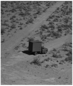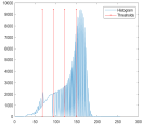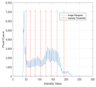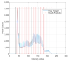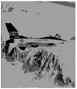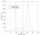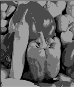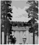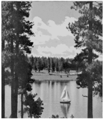Conventional approaches are limited by their reliance on assumptions, such as unimodality, continuity, and differentiability of the objective function, which rarely apply to non-linear systems [16]. Another important application is in image analysis, where image segmentation remains a critical and extensively researched task [17].

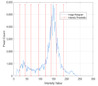
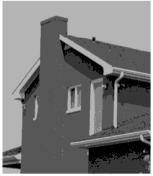
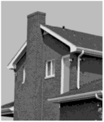
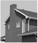
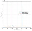
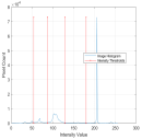
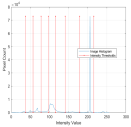
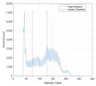
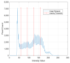
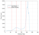
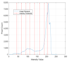
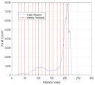
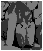
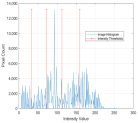
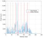
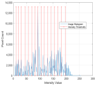
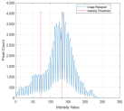
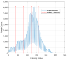
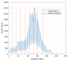
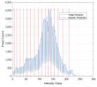
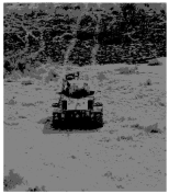
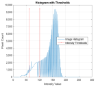
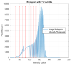
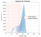
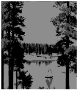
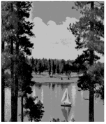
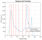
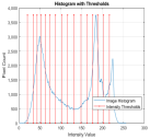
This process is a critical preliminary step in image analysis, aiming to divide an image into meaningful and homogeneous regions based on characteristics such as gray values, edge information, and texture. Framing this as an optimization problem involves minimizing the cross-entropy between the object and the background. However, this approach often encounters multiple local minima, complicating the computational process. Furthermore, the computational time grows exponentially with the number of thresholds, making it a challenging and resource-intensive task.

To address key limitations, particularly the high computational cost of threshold searches, numerous algorithms have been developed. In scenarios where traditional methods fall short, metaheuristic algorithms (MAs) offer a promising alternative. Unlike conventional approaches, MAs do not depend on simplifying assumptions such as unimodality, continuity, or differentiability, making them highly effective for complex nonlinear systems with multiple parameters and time-varying dynamics. Their success has been demonstrated in various real-world applications [16], including the identification of unknown parameters in biological models [18].

In this study, we propose a novel population-based algorithm, the Gaslike Social Motility Algorithm (GSM), for solving optimization problems. Inspired by the movement patterns of gas motility [19], GSM dynamically adapts its search process to efficiently explore the solution space. This model is characterized by its deterministic nature, minimal parameter requirements, and ability to replicate social behaviors, such as: (1) attraction between similar particles, (2) formation of stable groups, (3) division of groups into smaller units upon reaching a critical size, (4) modification of particle distributions through inter-group interactions during the search process, and (5) changes in particles’ internal states through local interactions. The proposed algorithm was evaluated using 22 benchmark optimization functions and compared against the performance of the PSO, DE, BA, ABC, AHA, AHA-AO, CBO, ECBO, and SNS algorithms. The GSM algorithm demonstrated superior performance, achieving optimal results for all benchmark functions with significantly fewer computational iterations than its counterparts.

The key contributions of this paper are: (1) the introduction of a novel swarm-based optimization algorithm, (2) a comprehensive comparison of various metaheuristic algorithms, and (3) the application of the proposed algorithm to image thresholding segmentation. These contributions underscore the significance of this work in advancing the field of metaheuristic algorithms (MAs).

The paper is structured as follows: first, the GSM algorithm is described in detail; next, a comparative analysis is conducted between GSM and state-of-the-art algorithms, including PSO, DE, BA, ABC, AHA, AHA-AO, CBO, ECBO, and SNS; then, the application of GSM to image thresholding segmentation is presented; and finally, the conclusions are discussed.

2. The Proposed Gaslike Social Motility (GSM) Algorithm

We propose a novel swarm-based algorithm for global optimization, inspired by the principles of gaslike social motility as described in [19].

This algorithm is based on the concept of collective movement, commonly observed in systems such as bird flocks, bee swarms, and animal herds. Each particle is characterized by an internal state that evolves through interactions with neighboring particles, where the interaction strength depends on the internal states of the neighbors. Specifically, a particle i responds to particle j by either approaching or retreating, requiring an evaluation of the local environment to determine the appropriate action.

The behavior of gas particles is described below, along with its adaptation to develop a global optimization strategy inspired by their dynamics.

2.1. Gaslike Social Motility Behavior: Inspiration and Application

In [19], each particle i interacts within a bounded, time-varying neighborhood defined by the proximity and affinity between the gas particle i and its surrounding particles. These interactions determine whether a particle i forms groups with its neighbors or moves away from them. The behavior of each particle is governed by the following dynamic rules:

$$x_{t+1}^i=(1-ϵ)f\left(x_t^i\right)+{\displaystyle \frac{ϵ}{|{\eta }_t^i|}}\sum _{j\in {\eta }_t^i}f\left(x_t^j\right),$$

(1)

$$r_{t+1}^i=r_t^i+\gamma \left(\sum _{j\in {\eta }_t^i}{\displaystyle \frac{r_t^j-r_t^i}{|r_t^j-r_t^i|}}\right)\left(x_{t+1}^i\sum _{j\in {\eta }_t^i}{x}_{t+1}^j\right).$$

(2)

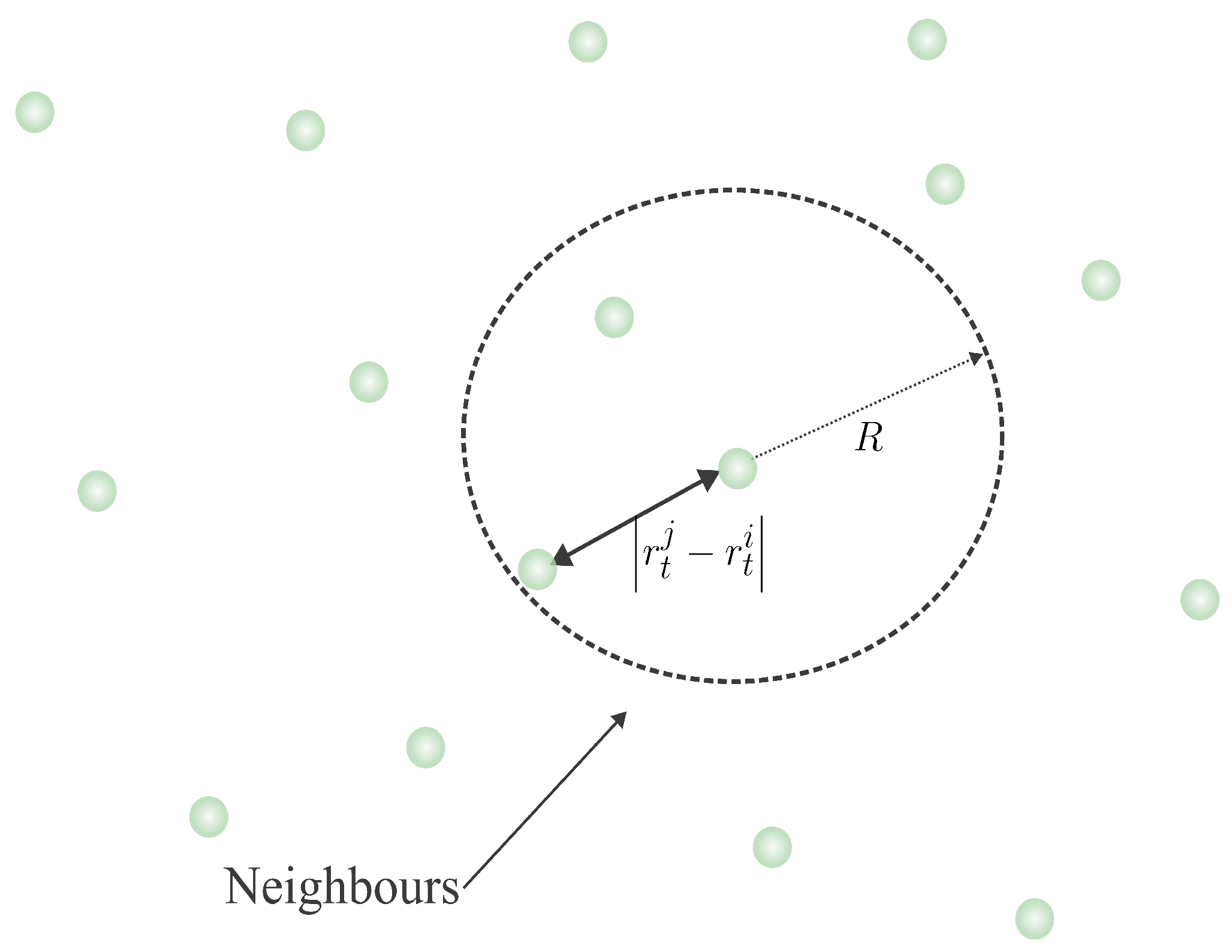
Here, $x_t^i$ denotes the feature (state or mood) of the i-th particle at the time step t, where i ranges from 1 to N, the total number of particles. The position vector ${\mathbf{r}}_t^i$ lies in a d-dimensional space, and the neighborhood of each particle is defined as ${\eta }_t^i=\{j:|{\mathbf{r}}_t^j-{\mathbf{r}}_t^i|\le R\}$, with $|{\eta }_t^i|$ representing its cardinality. The parameter $\gamma$ controls the coupling strength, determining how quickly a particle ${\mathbf{r}}_t^i$ adjusts its position to approach or retreat from others. The constant R defines the interaction radius for each particle, while $ϵ$ represents the bounded coupling strength within the range $0\le ϵ\le 1$.

The state of the particle $x_t^i$ is influenced not only by its own mood but also by the moods of its neighboring particles. The parameter $ϵ$ determines the extent of this influence: a higher value of $ϵ$ increases the contribution from neighbors, while a lower value diminishes it. This dynamic models a highly relevant social interaction mechanism, making it particularly suitable for application in metaheuristic algorithms.

In Equation (1), the function $f\left(x\right)$ governs the internal behavior of each particle and is applied across the entire network. The dynamics are coupled through a weighted sum of the influences exerted by the neighboring particles of the particle i. In this work, a network is defined as the set of relationships or connections that particles establish with their neighbors within their environment.

From Equation (2), it is clear that the particle i evaluates its environment globally before deciding whether to stay close to or move away from its neighbors. This decision is primarily determined by the two factors on the right-hand side of (2). The movement, which can be either inward or outward, is driven by the term $x_{t+1}^i{\sum }_{j\in {\eta }_t^i}{x}_{t+1}^j$. Here, particles exchange information about their “affinity” with their neighboring group, reflecting the similarity of their characteristics at time $t+1$. The direction of movement is influenced by the first factor in the equation, which assesses the angular distribution of neighbors relative to the particle i. Greater asymmetry in the angular distribution of neighbors results in a larger displacement magnitude for i.

2.2. Gaslike Social Motility Algorithm

The emergent behavior described by Equations (1) and (2) is well-suited for use as an optimization algorithm. To adapt this behavior for optimization, we introduced modifications while retaining the core principles of the original model. As a result, (1) and (2) are reformulated as follows:

$$x_{t+1}^i=(1-ϵ)f\left(r_t^i\right)+{\displaystyle \frac{ϵ}{|{\eta }_t^i|}}\sum _{j\in {\eta }_t^i}f\left(r_t^j\right),$$

(3)

$$r_{t+1}^i=r_{\mathcal{N}}+\gamma \left(\sum _{j\in {\eta }_t^j}{\displaystyle \frac{r_B^j-r_t^i}{|r_B^j-r_t^i|}}\right)\left(x_{t+1}^i\sum _{j\in {\eta }_t^j}{x}_{t+1}^j\right).$$

(4)

Here, we consider a population of N motile particles, each with a continuous position ${\mathbf{r}}_t^i\in {\mathbb{R}}^D$. Each particle i navigates the D-dimensional search space, where $x_t^i\in \mathbb{R}$ represents the state (or “mood”) of the i-th gas particle, reflecting its perception of the environment. The evolution of the particle’s state depends on its interactions with its neighborhood. In particular, when $r_B^j=r_t^i$, the best position achieved by the neighboring particle $r_B^j$ coincides with the position of particle $r_t^i$. In this case, the neighbor does not provide any meaningful contribution and is therefore ignored. Figure 1 illustrates an example of neighbor selection for the particle $r_t^i$ within the search space.

The primary objective is to optimize the function $f(·)$ by adjusting the position $\mathbf{r}$ of the gas particles. The optimization process depends entirely on the position $\mathbf{r}$ at the time step t, which is influenced by the particle’s mood $x_{t+1}^i$. The factor $x_{t+1}^i{\sum }_{j\in {\eta }_t^i}{x}_{t+1}^j$ is computed to determine the direction of motion for the particle.

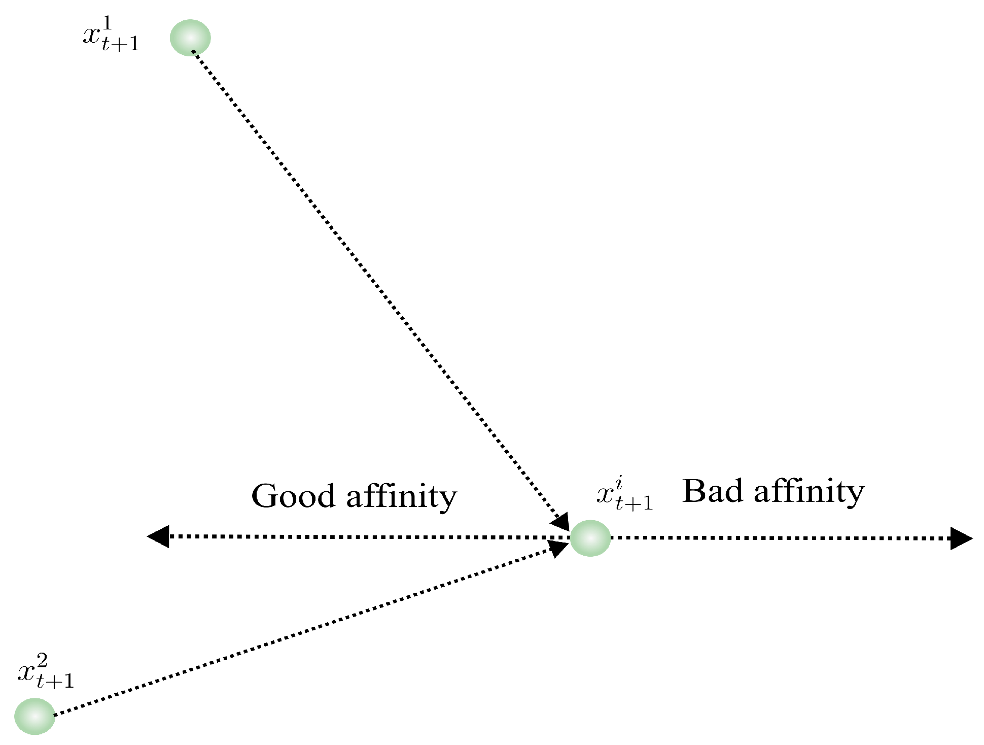
This equation quantifies the affinity of the particle i with its neighborhood. If the affinity is “good”, the particle i moves toward the dense region of the normal distribution corresponding to the best global position of the particles. If the affinity is “bad”, it moves in the opposite direction. Figure 2 illustrates whether the displacement is positive or negative based on the contributions of neighboring particles.

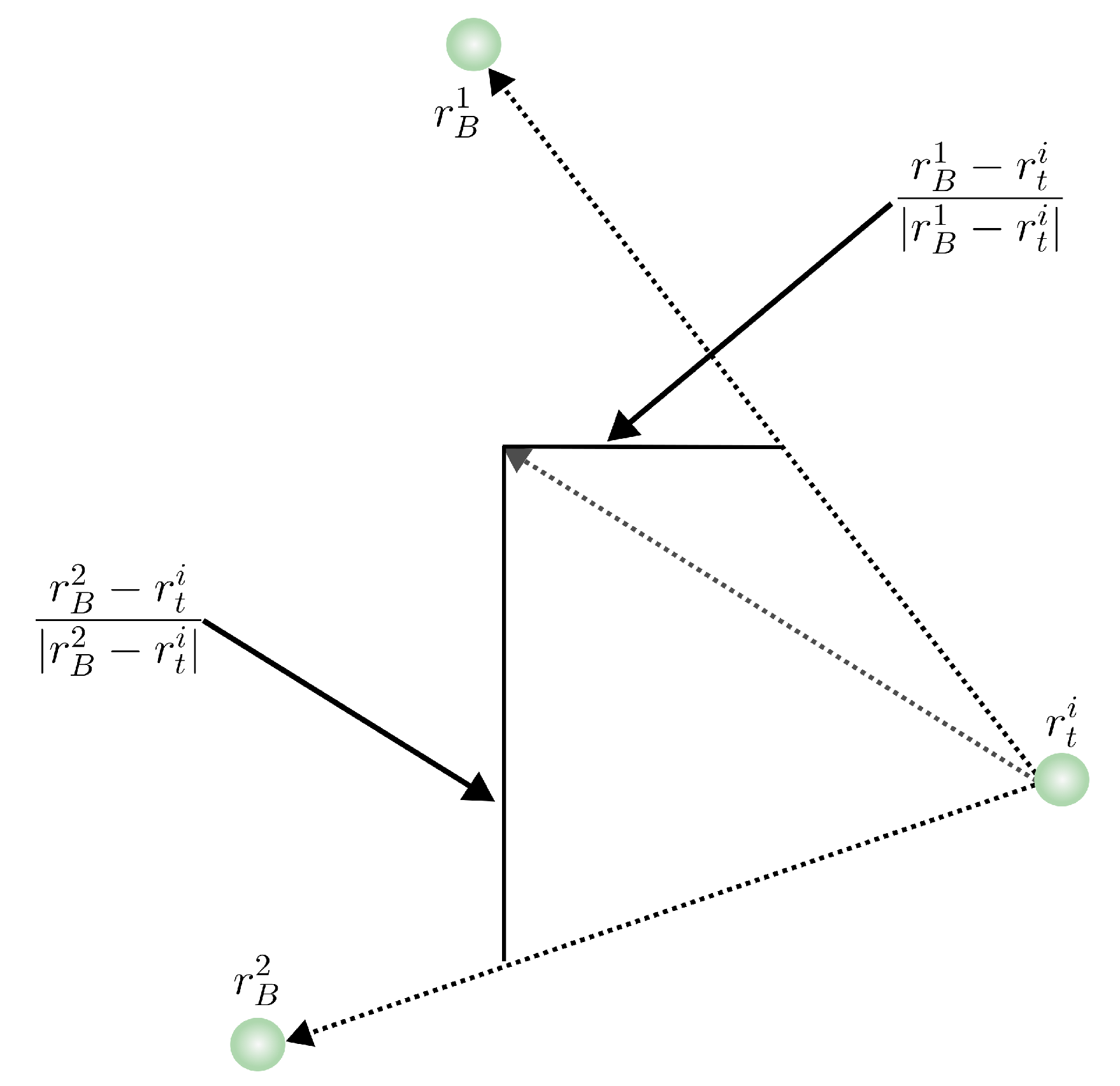
Moreover, in Equation (4), the direction of movement for particle i depends on the distribution of the best-visited positions ${\mathbf{r}}_B^j$ of all particles in the set ${\eta }_t^i$, relative to the position of i, as illustrated in Figure 3.

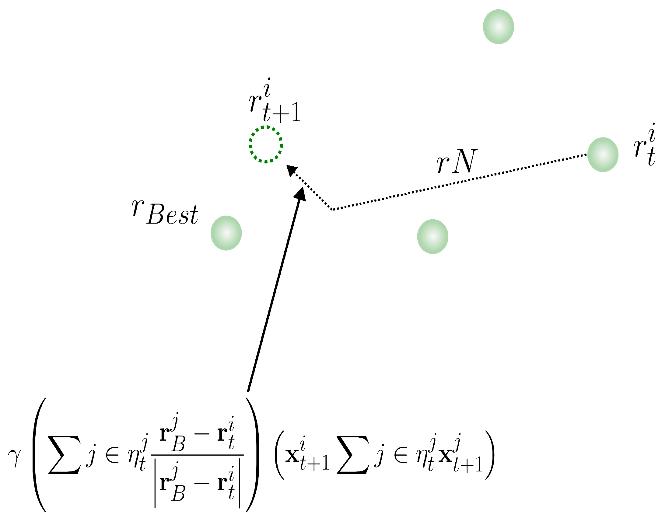
Finally, the term $r_{\mathcal{N}}$ is a vector generated as $r_{\mathcal{N}}\sim \mathcal{N}\left(r_{Best},{\sigma }_{bs}\right)$, where $r_{\mathcal{N}}=(r_1,r_2,\cdots ,r_D)\in {\mathbb{R}}^D$. This introduces a randomness factor that models the uncertainty and variability inherent in social systems, where particles may act unpredictably in response to external influences. In the context of the model, this term can produce effects contrary to expectations, generating deviations in particle displacement and reflecting behavioral diversity within the network. This reinforces the analogy to real social systems, where interactions between agents are not always deterministic. Here, $\mathcal{N}(·)$ is a normal distribution centered on the best global position ${\mathbf{r}}_{Best}$, and ${\sigma }_{bs}$ is the standard deviation of the best positions of $bs$ particles, where $bs<N$. This term represents the leadership of the best-performing particle, guiding collective movement toward feasible regions with optimal solutions. However, particles may choose to move closer or farther depending on interactions with nearby particles, as illustrated in Figure 4.

In summary, the displacement of the particles depends on how the position ${\mathbf{r}}^i$ relates to the best positions found by the set ${\eta }_t^i$ and how similar the next state ${\mathbf{x}}_{t+1}$ is to the corresponding i-th component. Specifically, if a particle is far from the best positions, it will move more significantly than if it is near them. The particle is attracted to remain in the vicinity of the best positions only if its state is comparable to those of its neighbors. If a particle has no neighbors (${\eta }_t^j\in \{\varnothing \}$), its position is determined solely by the random variable from $\mathcal{N}(·)$, and its internal state is defined by the objective function at ${\mathbf{r}}_t^i$. To avoid this scenario, an appropriate choice of R is crucial to ensure particles maintain interactions within the network, tailored to the properties of the objective function.

The selection of the parameters $ϵ$, $\gamma$, and R should be guided by the following considerations: $ϵ$ regulates the coupling between a particle’s internal state and that of its neighbors. Larger values ($0<ϵ<1$) increase the tendency to resemble neighboring particles, while $ϵ=0$ causes the particle to evolve independently of its neighborhood. $\gamma$ should be small enough to allow cluster formation, as $\gamma =0$ results in no motion. R depends on the size of the search space. If the space is large and R is small, particles may become too dispersed, preventing cluster formation. Conversely, if the space is small and R is large, particles will have nearly all others as neighbors. The interaction radius R defines the neighborhood size, and dynamically adjusting R allows the algorithm to balance local exploitation (small R) and global exploration (large R). When a particle has no useful neighbors (i.e., $r_B^j=r_t^i$), it acts independently, enabling it to escape local optima.

In this way, we preserve the original property, where individuals evaluate their internal state to determine how much they want to resemble their neighborhood and, in terms of position, how they are located relative to the best position of their neighbors and how similar they are to their surroundings.

Table 1. Summary of the parameters and variables in the Gaslike Social Motility (GSM) algorithm.

Symbol/Parameter	Meaning
N	Number of particles in the population
D	Dimensionality of the search space
G	Maximum number of generations
t	Iteration number
i	Index of a particle in the population ($i=1,2,\dots ,N$)
j	Index of a neighboring particle
$x_t^i$	State (mood) of particle i at time t
${\mathbf{r}}_t^i$	Position of particle i in a d-dimensional space
${\eta }_t^i$	Neighborhood of particle i at time t
$|{\eta }_t^i|$	Cardinality (size) of the neighborhood ${\eta }_t^i$
R	Interaction radius (defines the neighborhood size)
$ϵ$	Coupling strength
$\gamma$	Coupling factor
${\mathbf{r}}_B^j$	Best-known position of particle j
$r_{\mathcal{N}}$	Random displacement vector generated with a normal distribution
${\sigma }_{bs}$	Standard deviation of the best positions of $bs$ particles
$f(·)$	Objective function being optimized
$\mathcal{N}(·)$	Normal distribution function used for randomness
$x_{t+1}^i{\sum }_{j\in {\eta }_t^i}{x}_{t+1}^j$	Affinity factor determining the direction of movement

shows the list of GSM algorithm terms. The complete GSM algorithm is found in Algoritm 1.

Algorithm 1 GSM algorithm to solve minimization problems. f is the Objective Function, N the total number of particles and D the dimension of the problem.

1: R, $ϵ$, $\gamma$, $bs$← define parameters 2: $x^i$← initialize i ∈ N state of the particles randomly 3: $r^i$← initialize $i\in \{1,N\}$ random position such that $r^i\in {\mathbb{R}}^D$ 4: $r_B^i$←$r_t^i$, initialization of best particle positions 5: ${\eta }^i$ initialize $i\in \{N,N\}$ neighbors at zero such that ${\eta }^i\in {\mathbb{R}}^N$ 6: do 7:     for $i=1\to N$ do 8:         if $f\left(r_t^i\right)<f\left(r_B^i\right)$ then 9:            $r_B^i\leftarrow r_t^i$ 10:     Choose particle with best swarm position $r_{Best}$ 11:     Selection of the best particles bs from rt 12:     for $i=1\to N$ do 13:          $n\leftarrow 0$ 14:          for $j=1\to N$ do 15:              if $|{\mathbf{r}}_t^j-{\mathbf{r}}_t^i|\le R\&\&i\ne j$ then 16:                 ${\eta }_t^{i,n}\leftarrow j$ 17:                  $n\leftarrow n+1$ 18:     for $i=1\to N$ do 19:         ${\mathbf{x}}_{t+1}^i\leftarrow (1-ϵ)f\left({\mathbf{r}}_t^i\right)+{\displaystyle \frac{ϵ}{|{\eta }_t^i|}}{\sum }_{j\in {\eta }_t^i}f\left({\mathbf{r}}_t^j\right)$ 20: ${\mathbf{r}}_{t+1}^i\leftarrow r_{\mathcal{N}}+\gamma \left({\sum }_{j\in {\eta }_t^j}{\displaystyle \frac{{\mathbf{r}}_B^j-{\mathbf{r}}_t^i}{|{\mathbf{r}}_B^j-{\mathbf{r}}_t^i|}}\right)\left({\mathbf{x}}_{t+1}^i{\sum }_{j\in {\eta }_t^j}{\mathbf{x}}_{t+1}^j\right)$          $t=t+1$ 21: while Total number of iterations G is fulfilled

3. GSM Algorithm Performance Results

To evaluate the efficiency of the GSM algorithm, it was implemented and tested on a set of benchmark functions. The GSM algorithm was compared on equal terms with several well-known optimization algorithms, including PSO, DE, BA, ABC, AHA, AHA-AO, CBO, ECBO, and SNS. The benchmark functions were selected to represent a diverse range of problem types, such as unimodal, multimodal, regular, irregular, separable, non-separable, and multidimensional functions. The parameters used for each algorithm in this study are provided in Table 2.

A unimodal function has a single global optimum with no or only one local optimum, while a multimodal function features multiple local optima. Optimization algorithms are often tested on multimodal functions to assess their ability to avoid local optima. Algorithms with poor exploration capabilities may struggle to search the space thoroughly and may converge to suboptimal solutions. Additionally, flat search spaces pose challenges as they lack gradient information to guide the algorithm toward the global optimum [20]. Both separable and non-separable functions were included in the tests to further evaluate algorithm performance [20].

High-dimensional search spaces present another significant challenge for optimization algorithms. As the dimensionality of a problem increases, the search space volume grows exponentially, making it harder to locate the global optimum. Algorithms that perform well in low-dimensional spaces may struggle in high-dimensional environments. Therefore, global optimization algorithms are rigorously tested in high-dimensional search spaces to ensure robustness [21].

Scaling problems also pose difficulties for optimization algorithms. These problems involve significant variations in magnitude between the domain and the frequency of the hypersurface, complicating the search process [22]. For instance, Langerman functions are nonsymmetrical with randomly distributed local optima, making them particularly challenging to optimize. The quartic function introduces random noise (Gaussian or uniform), requiring algorithms to handle noisy data effectively. Algorithms that fail to perform well on noisy functions are likely to struggle in real-world applications where noise is prevalent. The benchmark functions used in this study are summarized in Table 3 and Table 4, categorized by unimodal and multimodal functions, respectively. These functions are further classified based on characteristics such as continuity, separability, scalability, and differentiability.

The GSM algorithm was compared against PSO, DE, BA, ABC, AHA, AHA-AO, CBO, ECBO, and SNS using the 22 benchmark functions listed in Table 3 and Table 4. Each algorithm was executed 100 times, and the mean, standard deviation, and optimal values were recorded. The number of iterations and population size for each algorithm are detailed in Table 3 and Table 4. All algorithms were implemented in MATLAB 24.2.0.2871072 (R2024b) Update 5 (The MathWorks, Inc., Natick, MA, USA), and the results are presented in Table 5 and Table 6. The findings indicate that the GSM algorithm converges to optimal values with high precision, requiring fewer iterations and smaller population sizes compared to other algorithms.

In Table 7, a ‘‘+’’ denotes cases where the GSM algorithm outperformed the other algorithms in terms of mean values, while a ‘‘−’’ indicates inferior performance. Overall, the GSM algorithm demonstrated superior performance on most benchmark functions compared to PSO, DE, BA, ABC, AHA, AHA-AO, CBO, ECBO, and SNS.

Table 2. Parameters of the algorithms.

Algorithm	Parameters	Reference
GSM	$R=0.1$, $\epsilon =0.0001$ $\gamma =0.001$$bs=5$
PSO	$c_1=2.0$, $c_2=2.0$, and $\omega =0.9-0.2$	[23]
DE	$F=0.9$ and $cr=0.2$	[24]
BA	$f_{min}=0$,$f_{max}=1$, $A_0=1$, $r_0=0.1$, $\alpha =0.9$,$\gamma =0.9$	[25]
ABC	Food sources = 10	[20]
AHA	$Mi{g}_{trigger}=20$, Flight Step size $F_{sz}=[-1,1]$ and $r\in [0,1]$	[8]
CBO	no parameters	[9]
ECBO	$Pro=0.5$	[10]
AHA-AO	$\alpha =0.1$,$\delta =0.1$, $\omega =0.005$ and $r\in [0,1]$	[11]
SNS	no parameters	[12]

Table 2. Parameters of the algorithms.

Algorithm	Parameters	Reference
GSM	$R=0.1$, $\epsilon =0.0001$ $\gamma =0.001$$bs=5$
PSO	$c_1=2.0$, $c_2=2.0$, and $\omega =0.9-0.2$	[23]
DE	$F=0.9$ and $cr=0.2$	[24]
BA	$f_{min}=0$,$f_{max}=1$, $A_0=1$, $r_0=0.1$, $\alpha =0.9$,$\gamma =0.9$	[25]
ABC	Food sources = 10	[20]
AHA	$Mi{g}_{trigger}=20$, Flight Step size $F_{sz}=[-1,1]$ and $r\in [0,1]$	[8]
CBO	no parameters	[9]
ECBO	$Pro=0.5$	[10]
AHA-AO	$\alpha =0.1$,$\delta =0.1$, $\omega =0.005$ and $r\in [0,1]$	[11]
SNS	no parameters	[12]

Table 3. Unimodal benchmark functions used in experiments F, the number of iterations I, population P, and dimension D.

No	Function (F)	Type	D	Range	Formulation	P	I
$F_1$	BOOTH	U, C, Di, NS, NSc	2	[−10, 10]	$f\left(x\right)={(x_1+2x_2-7)}^2+{(2x_1+x_2-5)}^2$	50	100
$F_2$	SPHERE	U, S	2	[−5.12, 5.12]	$f\left(x\right)={\sum }_{i=1}^d{x}_i^2$	50	50
$F_3$	SPHERE	U, S	10	[−5.12, 5.12]	$f\left(x\right)={\sum }_{i=1}^d{x}_i^2$	150	100
$F_4$	SPHERE	U, S	20	[−5.12, 5.12]	$f\left(x\right)={\sum }_{i=1}^d{x}_i^2$	150	150
$F_5$	BEALE	U, C, Di, NS, NSc, S	2	[−4.5, 4.5]	$\begin{array}{c}f\left(x\right)=\\ {(1.5-x_1+x_1{x}_2)}^2+\\ {(2.25-x_1+x_1{x}_2^2)}^2+\\ {(2.625-x_1+x_2^3)}^2\end{array}$	50	100
$F_6$	ROTATED HYPER-ELLIPSOID	U, C, Di, NS, NSc	2	[−65.536, 65.536]	$f\left(x\right)={\sum }_{i=1}^d{\sum }_{j=1}^i{x}_j^2$	50	250
$F_7$	SUM SQUARES	U, C, Di, S, Sc	20	[−5.12, 5.12]	$f\left(x\right)={\sum }_{i=1}^{d}i{x}_i^2$	200	500
$F_8$	QUARTIC	U, C, Di, S, Sc	2	[−1.28, 1.28]	$\begin{array}{c}f\left(x\right)=f(x_1,\dots .,x_n)=\\ {\sum }_{i=1}^{n}i{x}_i^4+\\ random[0,1)\end{array}$	50	100

Table 3. Unimodal benchmark functions used in experiments F, the number of iterations I, population P, and dimension D.

No	Function (F)	Type	D	Range	Formulation	P	I
$F_1$	BOOTH	U, C, Di, NS, NSc	2	[−10, 10]	$f\left(x\right)={(x_1+2x_2-7)}^2+{(2x_1+x_2-5)}^2$	50	100
$F_2$	SPHERE	U, S	2	[−5.12, 5.12]	$f\left(x\right)={\sum }_{i=1}^d{x}_i^2$	50	50
$F_3$	SPHERE	U, S	10	[−5.12, 5.12]	$f\left(x\right)={\sum }_{i=1}^d{x}_i^2$	150	100
$F_4$	SPHERE	U, S	20	[−5.12, 5.12]	$f\left(x\right)={\sum }_{i=1}^d{x}_i^2$	150	150
$F_5$	BEALE	U, C, Di, NS, NSc, S	2	[−4.5, 4.5]	$\begin{array}{c}f\left(x\right)=\\ {(1.5-x_1+x_1{x}_2)}^2+\\ {(2.25-x_1+x_1{x}_2^2)}^2+\\ {(2.625-x_1+x_2^3)}^2\end{array}$	50	100
$F_6$	ROTATED HYPER-ELLIPSOID	U, C, Di, NS, NSc	2	[−65.536, 65.536]	$f\left(x\right)={\sum }_{i=1}^d{\sum }_{j=1}^i{x}_j^2$	50	250
$F_7$	SUM SQUARES	U, C, Di, S, Sc	20	[−5.12, 5.12]	$f\left(x\right)={\sum }_{i=1}^{d}i{x}_i^2$	200	500
$F_8$	QUARTIC	U, C, Di, S, Sc	2	[−1.28, 1.28]	$\begin{array}{c}f\left(x\right)=f(x_1,\dots .,x_n)=\\ {\sum }_{i=1}^{n}i{x}_i^4+\\ random[0,1)\end{array}$	50	100

The GSM algorithm demonstrates superior performance on unimodal, continuous, differentiable, nonseparable, and nonscalable functions $F_1$, $F_5$, and $F_6$, outperforming the compared algorithms, including the most recent ones in the literature. Notably, for $F_1$, the GSM algorithm consistently finds the global optimum with few iterations. For unimodal and separable functions such as $F_2$, $F_3$, and $F_4$, algorithms like AHA, AHA-AO, and SNS exhibit better performance in high-dimensional spaces, indicating their ability to converge quickly on smooth functions. However, in low-dimensional settings, the GSM algorithm shows a slight improvement over these algorithms. Functions $F_7$ and $F_8$ are unimodal, continuous, differentiable, separable, and scalable. For $F_7$, the AHA, AHA-AO, and SNS algorithms achieve the best results. In the case of $F_8$, the GSM, AHA, AHA-AO, and SNS algorithms perform similarly, making it difficult to determine which algorithm is superior for this function.

Table 4. Multimodal benchmark functions used in experiments F, the number of iterations I, population P, and dimension D.

No	Function (F)	Type	D	Range	Formulation	P	I
$F_9$	SIX-HUMP CAMEL	M, C, Di, NS, NSc	2	[−3, 3], [−2, 2]	$f\left(x\right)=\left(4-2.1x_1^2+{\displaystyle \frac{x_1^4}{3}}\right)x_1^2+x_1{x}_2+(-4+4x_2^2)x_2^2$	15	20
$F_{10}$	ACKLEY	M, C, Di, NS, Sc	2	[−32.768, 32.768]	$f\left(x\right)=-aexp\left(-b\sqrt{{\displaystyle \frac{1}{d}}{\sum }_{i=1}^d{x}_i^2}\right)-exp\left({\displaystyle \frac{1}{d}}{\sum }_{i=1}^{d}cos\left(c{x}_i\right)\right)+a+exp\left(1\right)$	50	100
$F_{11}$	MICHALEWICZ	M, S	2	[0, $\pi$]	$f\left(x\right)=-{\sum }_{i=1}^{d}sin\left(x_i\right)si{n}^{2m}\left({\displaystyle \frac{i{x}_i^2}{\pi }}\right)$	50	15
$F_{12}$	MICHALEWICZ	M, S	5	[0, $\pi$]	$f\left(x\right)=-{\sum }_{i=1}^{d}sin\left(x_i\right)si{n}^{2m}\left({\displaystyle \frac{i{x}_i^2}{\pi }}\right)$	200	100
$F_{13}$	MICHALEWICZ	M, S	10	[0, $\pi$]	$f\left(x\right)=-{\sum }_{i=1}^{d}sin\left(x_i\right)si{n}^{2m}\left({\displaystyle \frac{i{x}_i^2}{\pi }}\right)$	150	40
$F_{14}$	GRIEWANK	M, C, Di, NS, Sc	2	[−600, 600]	$f\left(x\right)={\sum }_{i=1}^d{\displaystyle \frac{x_i^2}{4000}}-{\prod }_{i=1}^{d}cos\left({\displaystyle \frac{x_i}{\sqrt{i}}}\right)+1$	150	100
$F_{15}$	CROSS-IN-TRAY	M, C, NS, NSc	2	[-10, 10]	$f\left(x\right)=-0.0001{\left(\left|sin\left(x_1\right)sin\left(x_2\right)exp\left(|100-{\displaystyle \frac{\sqrt{x_1^2+x_2^2}}{\pi }}|\right)\right|+1\right)}^{0.1}$	50	15
$F_{16}$	LEVY	M, NS	5	[−10, 10]	$f\left(x\right)=si{n}^2\left(\pi w_1\right)+{\sum }_{i=1}^{d-1}{(w_i-1)}^2[1+10si{n}^2(\pi w_i+1)]+{(w_d-1)}^2[1+si{n}^2\left(2\pi w_d\right)],$	50	100
					where $w_i=1+{\displaystyle \frac{x_i-1}{4}},$for all $i=1,...,d$
$F_{17}$	EASOM	M, C, Di, S, NSc	2	[-$100,100]$	$f\left(x\right)=-cos\left(x_1\right)cos\left(x_2\right)exp\left(-{(x_1-\pi )}^2-{(x_2-\pi )}^2\right)$	50	25
$F_{18}$	BRANIN	M, C, Di, NS, NSc	2	[−5, 10], [0, 15]	$f\left(x\right)=a{(x_2-b{x}_1^2+c{x}_1-r)}^2+s(1-t)cos\left(x_1\right)+s$	50	15
$F_{19}$	BOHACHEVSKY	M, C, Di, S, NSc	2	[−100, 100]	$f_1\left(x\right)=x_1^2+2x_2^2-0.3cos\left(3\pi x_1\right)-0.4cos\left(4\pi x_2\right)+0.7$	50	50
$F_{20}$	SCHWEFEL	M, C, Di, S, Sc	2	[−500, 500]	$f\left(X\right)=418.9829d-{\sum }_{i=1}^d{x}_{i}sin\left(\sqrt{|x_i|}\right)$	50	100
$F_{21}$	SHUBERT	M, C, Di, S, NSc	2	[−10, 10]	$f\left(x\right)=\left({\sum }_{i=1}^{5}icos((i+1)x_1+i)\right)\left({\sum }_{i=1}^{5}icos((i+1)x_2+i)\right)$	50	50
$F_{22}$	LANGERMANN	M, NS	2	[0, 10]	$f\left(x\right)={\sum }_{i=1}^m{c}_{i}exp\left(-{\displaystyle \frac{1}{\pi }}{\sum }_{j=1}^d{(x_j-A_{ij})}^2\right)cos\left(\pi {\sum }_{j=1}^d{(x_j-A_{ij})}^2\right)$	50	100

Table 4. Multimodal benchmark functions used in experiments F, the number of iterations I, population P, and dimension D.

No	Function (F)	Type	D	Range	Formulation	P	I
$F_9$	SIX-HUMP CAMEL	M, C, Di, NS, NSc	2	[−3, 3], [−2, 2]	$f\left(x\right)=\left(4-2.1x_1^2+{\displaystyle \frac{x_1^4}{3}}\right)x_1^2+x_1{x}_2+(-4+4x_2^2)x_2^2$	15	20
$F_{10}$	ACKLEY	M, C, Di, NS, Sc	2	[−32.768, 32.768]	$f\left(x\right)=-aexp\left(-b\sqrt{{\displaystyle \frac{1}{d}}{\sum }_{i=1}^d{x}_i^2}\right)-exp\left({\displaystyle \frac{1}{d}}{\sum }_{i=1}^{d}cos\left(c{x}_i\right)\right)+a+exp\left(1\right)$	50	100
$F_{11}$	MICHALEWICZ	M, S	2	[0, $\pi$]	$f\left(x\right)=-{\sum }_{i=1}^{d}sin\left(x_i\right)si{n}^{2m}\left({\displaystyle \frac{i{x}_i^2}{\pi }}\right)$	50	15
$F_{12}$	MICHALEWICZ	M, S	5	[0, $\pi$]	$f\left(x\right)=-{\sum }_{i=1}^{d}sin\left(x_i\right)si{n}^{2m}\left({\displaystyle \frac{i{x}_i^2}{\pi }}\right)$	200	100
$F_{13}$	MICHALEWICZ	M, S	10	[0, $\pi$]	$f\left(x\right)=-{\sum }_{i=1}^{d}sin\left(x_i\right)si{n}^{2m}\left({\displaystyle \frac{i{x}_i^2}{\pi }}\right)$	150	40
$F_{14}$	GRIEWANK	M, C, Di, NS, Sc	2	[−600, 600]	$f\left(x\right)={\sum }_{i=1}^d{\displaystyle \frac{x_i^2}{4000}}-{\prod }_{i=1}^{d}cos\left({\displaystyle \frac{x_i}{\sqrt{i}}}\right)+1$	150	100
$F_{15}$	CROSS-IN-TRAY	M, C, NS, NSc	2	[-10, 10]	$f\left(x\right)=-0.0001{\left(\left|sin\left(x_1\right)sin\left(x_2\right)exp\left(|100-{\displaystyle \frac{\sqrt{x_1^2+x_2^2}}{\pi }}|\right)\right|+1\right)}^{0.1}$	50	15
$F_{16}$	LEVY	M, NS	5	[−10, 10]	$f\left(x\right)=si{n}^2\left(\pi w_1\right)+{\sum }_{i=1}^{d-1}{(w_i-1)}^2[1+10si{n}^2(\pi w_i+1)]+{(w_d-1)}^2[1+si{n}^2\left(2\pi w_d\right)],$	50	100
					where $w_i=1+{\displaystyle \frac{x_i-1}{4}},$for all $i=1,...,d$
$F_{17}$	EASOM	M, C, Di, S, NSc	2	[-$100,100]$	$f\left(x\right)=-cos\left(x_1\right)cos\left(x_2\right)exp\left(-{(x_1-\pi )}^2-{(x_2-\pi )}^2\right)$	50	25
$F_{18}$	BRANIN	M, C, Di, NS, NSc	2	[−5, 10], [0, 15]	$f\left(x\right)=a{(x_2-b{x}_1^2+c{x}_1-r)}^2+s(1-t)cos\left(x_1\right)+s$	50	15
$F_{19}$	BOHACHEVSKY	M, C, Di, S, NSc	2	[−100, 100]	$f_1\left(x\right)=x_1^2+2x_2^2-0.3cos\left(3\pi x_1\right)-0.4cos\left(4\pi x_2\right)+0.7$	50	50
$F_{20}$	SCHWEFEL	M, C, Di, S, Sc	2	[−500, 500]	$f\left(X\right)=418.9829d-{\sum }_{i=1}^d{x}_{i}sin\left(\sqrt{|x_i|}\right)$	50	100
$F_{21}$	SHUBERT	M, C, Di, S, NSc	2	[−10, 10]	$f\left(x\right)=\left({\sum }_{i=1}^{5}icos((i+1)x_1+i)\right)\left({\sum }_{i=1}^{5}icos((i+1)x_2+i)\right)$	50	50
$F_{22}$	LANGERMANN	M, NS	2	[0, 10]	$f\left(x\right)={\sum }_{i=1}^m{c}_{i}exp\left(-{\displaystyle \frac{1}{\pi }}{\sum }_{j=1}^d{(x_j-A_{ij})}^2\right)cos\left(\pi {\sum }_{j=1}^d{(x_j-A_{ij})}^2\right)$	50	100

On the other hand, functions $F_9$ and $F_{18}$ are multimodal, continuous, differentiable, non-separable, and non-scalable, featuring multiple local minima. For these functions, the GSM algorithm achieves the best results with a low standard deviation, indicating high precision. Functions $F_{10}$ and $F_{14}$ are multimodal, continuous, differentiable, non-separable, and scalable. For $F_{10}$, the GSM algorithm performs slightly better than the other algorithms. However, for $F_{14}$, the AHA and AHA-AO algorithms demonstrate superior performance. Functions $F_{11}$, $F_{12}$, and $F_{13}$ are multimodal and separable, posing challenges for all algorithms in locating the global optimum. For $F_{11}$ and $F_{13}$, the GSM algorithm produces results closest to the optimum, while for $F_{12}$, the DE algorithm outperforms the others. For the non-scalable function $F_{15}$, the GSM algorithm surpasses all competing algorithms. Similarly, for $F_{16}$, a multimodal and non-separable function, the GSM algorithm proves to be the best. In the case of $F_{17}$, a continuous, differentiable, non-scalable, and multimodal function, both the GSM and ABC algorithms deliver strong results, with GSM performing slightly better. Functions $F_{19}$ and $F_{21}$ are multimodal, continuous, separable, non-scalable, and differentiable. While most algorithms perform well on these functions, the GSM algorithm stands out as the best. In contrast, $F_{20}$ is a scalable function where all algorithms struggle to find the optimum, with the best results achieved by SNS, AHA, AHA-AO, and GSM. Finally, for $F_{22}$, a multimodal and non-separable function, most algorithms fail to optimize effectively. However, the closest results to the optimum are obtained by CBO, ECBO, and GSM.

Table 5. Results of all proposed algorithms for unimodal functions.

No	$\mathbf{Min}$		GSM	PSO	DE	BA	ABC	AHA	CBO	ECBO	AHA-AO	SNS
$F_1$	0	Best	0	4.7161 $\times {10}^{-4}$	1.5620 $\times {10}^{-15}$	1.9285 $\times {10}^{-23}$	5.4342 $\times {10}^{-17}$	2.2249 $\times {10}^{-9}$	2.1592 $\times {10}^{-20}$	1.4831 $\times {10}^{-5}$	1.0684 $\times {10}^{-8}$	7.2601 $\times {10}^{-21}$
		Mean	0	3.3472 $\times {10}^{-8}$	6.2692 $\times {10}^{-12}$	8.4600 $\times {10}^{-20}$	5.8342 $\times {10}^{-13}$	1.5434 $\times {10}^{-9}$	2.1668 $\times {10}^{-18}$	8.3649 $\times {10}^{-5}$	3.9487$\times {10}^{-9}$	8.1263 $\times {10}^{-19}$
		StdDev	0	1.0584 $\times {10}^{-7}$	1.7007 $\times {10}^{-11}$	9.9731 $\times {10}^{-20}$	1.7111 $\times {10}^{-12}$	2.5825 $\times {10}^{-9}$	4.6605 $\times {10}^{-18}$	1.0683 $\times {10}^{-4}$	3.4400 $\times {10}^{-9}$	1.2731 $\times {10}^{-18}$
$F_2$	0	Best	7.0223 $\times {10}^{-47}$	5.211 $\times {10}^{-4}$	6.6253 $\times {10}^{-18}$	2.3480 $\times {10}^{-15}$	8.1189 $\times {10}^{-11}$	4.0049 $\times {10}^{-19}$	1.8585 $\times {10}^{-13}$	1.0575 $\times {10}^{-6}$	2.9348 $\times {10}^{-13}$	1.8608 $\times {10}^{-18}$
		Mean	4.8067 $\times {10}^{-37}$	1.0242 $\times {10}^{-8}$	1.6800 $\times {10}^{-16}$	3.6863 $\times {10}^{-14}$	3.1458 $\times {10}^{-8}$	3.3871 $\times {10}^{-18}$	1.4750 $\times {10}^{-13}$	1.2829 $\times {10}^{-5}$	5.8306 $\times {10}^{-11}$	4.2709 $\times {10}^{-17}$
		StdDev	1.5200 $\times {10}^{-36}$	3.2126 $\times {10}^{-8}$	1.4829 $\times {10}^{-16}$	3.9603 $\times {10}^{-14}$	5.4034 $\times {10}^{-8}$	4.6770 $\times {10}^{-18}$	2.3268 $\times {10}^{-13}$	1.3716 $\times {10}^{-5}$	1.5306 $\times {10}^{-10}$	8.0683 $\times {10}^{-17}$
$F_3$	0	Best	1.8983 $\times {10}^{-23}$	1.2195 $\times {10}^{-10}$	3.2206 $\times {10}^{-6}$	2.6370 $\times {10}^{-12}$	0.0143	2.2838 $\times {10}^{-28}$	2.6720 $\times {10}^{-5}$	0.0144	1.5281 $\times {10}^{-25}$	4.3313 $\times {10}^{-19}$
		Mean	5.5377 $\times {10}^{-23}$	3.0311 $\times {10}^{-7}$	5.6897 $\times {10}^{-6}$	3.7566 $\times {10}^{-11}$	0.0303	2.9439 $\times {10}^{-28}$	2.6527 $\times {10}^{-5}$	0.0170	4.3047 $\times {10}^{-20}$	3.5935 $\times {10}^{-19}$
		StdDev	6.4917 $\times {10}^{-23}$	6.1127 $\times {10}^{-7}$	1.8035 $\times {10}^{-6}$	3.7826 $\times {10}^{-11}$	0.0189	6.7651 $\times {10}^{-28}$	1.1917 $\times {10}^{-5}$	0.0060	8.1642 $\times {10}^{-20}$	2.3942 $\times {10}^{-19}$
$F_4$	0	Best	5.4565 $\times {10}^{-19}$	9.0912 $\times {10}^{-10}$	1.0301 $\times {10}^{-4}$	7.9196 $\times {10}^{-9}$	0.1569	1.0626 $\times {10}^{-50}$	0.0039	0.1433	1.0605 $\times {10}^{-36}$	2.3915 $\times {10}^{-25}$
		Mean	4.4192 $\times {10}^{-8}$	2.4432 $\times {10}^{-5}$	1.8558 $\times {10}^{-4}$	2.6131 $\times {10}^{-8}$	0.4346	8.8246 $\times {10}^{-44}$	0.0090	0.1320	3.9312 $\times {10}^{-30}$	1.1474 $\times {10}^{-25}$
		StdDev	1.3878 $\times {10}^{-7}$	3.9384 $\times {10}^{-5}$	6.3749 $\times {10}^{-5}$	1.0577 $\times {10}^{-8}$	0.2315	1.3711 $\times {10}^{-43}$	0.0027	0.0457	1.0593 $\times {10}^{-29}$	6.7661 $\times {10}^{-26}$
$F_5$	0	Best	0	2.6321 $\times {10}^{-16}$	8.9583 $\times {10}^{-13}$	5.7992 $\times {10}^{-21}$	2.9569 $\times {10}^{-15}$	2.1248 $\times {10}^{-10}$	9.5145 $\times {10}^{-12}$	2.9519 $\times {10}^{-6}$	3.6675 $\times {10}^{-11}$	1.0593 $\times {10}^{-16}$
		Mean	2.7733 $\times {10}^{-33}$	9.6230 $\times {10}^{-4}$	5.2257 $\times {10}^{-10}$	0.0909	6.9116 $\times {10}^{-13}$	7.7244 $\times {10}^{-10}$	1.3407 $\times {10}^{-9}$	2.2842 $\times {10}^{-5}$	2.8535 $\times {10}^{-10}$	1.7591 $\times {10}^{-14}$
		StdDev	8.7700 $\times {10}^{-33}$	0.0030	1.2922 $\times {10}^{-9}$	0.1917	1.4852 $\times {10}^{-12}$	1.0677 $\times {10}^{-9}$	3.3844 $\times {10}^{-9}$	5.1538 $\times {10}^{-5}$	4.5641 $\times {10}^{-10}$	5.1523 $\times {10}^{-14}$
$F_6$	0	Best	6.0353 $\times {10}^{-228}$	1.2180 $\times {10}^{-62}$	1.6365 $\times {10}^{-80}$	3.8400 $\times {10}^{-32}$	3.6787 $\times {10}^{-41}$	4.3497 $\times {10}^{-91}$	5.1664 $\times {10}^{-64}$	2.8114 $\times {10}^{-6}$	2.7457 $\times {10}^{-64}$	8.2010 $\times {10}^{-76}$
		Mean	3.0077 $\times {10}^{-226}$	7.3249 $\times {10}^{-53}$	4.9137 $\times {10}^{-76}$	9.9511 $\times {10}^{-29}$	2.2754 $\times {10}^{-38}$	3.8621 $\times {10}^{-83}$	4.8796 $\times {10}^{-62}$	2.3092 $\times {10}^{-5}$	2.4815 $\times {10}^{-57}$	2.8823 $\times {10}^{-74}$
		StdDev	0	2.1958 $\times {10}^{-52}$	1.0362 $\times {10}^{-75}$	2.8837 $\times {10}^{-28}$	5.0686 $\times {10}^{-38}$	6.6999 $\times {10}^{-83}$	7.6559 $\times {10}^{-62}$	2.6735 $\times {10}^{-5}$	7.2763 $\times {10}^{-57}$	7.6906 $\times {10}^{-74}$
$F_7$	0	Best	4.6778 $\times {10}^{-60}$	9.7328 $\times {10}^{-24}$	4.4776 $\times {10}^{-17}$	3.0762 $\times {10}^{-13}$	0.6562	2.4692 $\times {10}^{-152}$	1.9993 $\times {10}^{-12}$	0.0678	1.7838 $\times {10}^{-116}$	3.5424 $\times {10}^{-85}$
		Mean	5.9890 $\times {10}^{-59}$	5.7186 $\times {10}^{-22}$	6.9886 $\times {10}^{-17}$	8.4214 $\times {10}^{-10}$	2.1627	2.8594 $\times {10}^{-152}$	6.7964 $\times {10}^{-12}$	0.1077	5.1417 $\times {10}^{-100}$	1.0878 $\times {10}^{-85}$
		StdDev	1.0477 $\times {10}^{-58}$	1.5996 $\times {10}^{-21}$	2.2506 $\times {10}^{-17}$	2.1557 $\times {10}^{-9}$	1.1511	7.9217 $\times {10}^{-152}$	3.4927 $\times {10}^{-12}$	0.0610	1.6259 $\times {10}^{-99}$	1.0818 $\times {10}^{-85}$
$F_8$	0	Best	8.9795 $\times {10}^{-5}$	0.0188	4.7591 $\times {10}^{-4}$	9.5197 $\times {10}^{-5}$	0.5218	0.000604	2.8205 $\times {10}^{-4}$	0.0021	0.0013	4.1045 $\times {10}^{-4}$
		Mean	6.1556 $\times {10}^{-4}$	0.0192	0.0011	0.0119	0.3278	5.5981 $\times {10}^{-4}$	5.8584 $\times {10}^{-4}$	0.0018	6.1085 $\times {10}^{-4}$	5.7738 $\times {10}^{-4}$
		StdDev	6.9240 $\times {10}^{-4}$	0.0125	7.2484 $\times {10}^{-4}$	0.0228	0.0642	3.2712 $\times {10}^{-4}$	2.9234 $\times {10}^{-4}$	0.0016	7.7823 $\times {10}^{-4}$	6.8678 $\times {10}^{-4}$

Table 5. Results of all proposed algorithms for unimodal functions.

No	$\mathbf{Min}$		GSM	PSO	DE	BA	ABC	AHA	CBO	ECBO	AHA-AO	SNS
$F_1$	0	Best	0	4.7161 $\times {10}^{-4}$	1.5620 $\times {10}^{-15}$	1.9285 $\times {10}^{-23}$	5.4342 $\times {10}^{-17}$	2.2249 $\times {10}^{-9}$	2.1592 $\times {10}^{-20}$	1.4831 $\times {10}^{-5}$	1.0684 $\times {10}^{-8}$	7.2601 $\times {10}^{-21}$
		Mean	0	3.3472 $\times {10}^{-8}$	6.2692 $\times {10}^{-12}$	8.4600 $\times {10}^{-20}$	5.8342 $\times {10}^{-13}$	1.5434 $\times {10}^{-9}$	2.1668 $\times {10}^{-18}$	8.3649 $\times {10}^{-5}$	3.9487$\times {10}^{-9}$	8.1263 $\times {10}^{-19}$
		StdDev	0	1.0584 $\times {10}^{-7}$	1.7007 $\times {10}^{-11}$	9.9731 $\times {10}^{-20}$	1.7111 $\times {10}^{-12}$	2.5825 $\times {10}^{-9}$	4.6605 $\times {10}^{-18}$	1.0683 $\times {10}^{-4}$	3.4400 $\times {10}^{-9}$	1.2731 $\times {10}^{-18}$
$F_2$	0	Best	7.0223 $\times {10}^{-47}$	5.211 $\times {10}^{-4}$	6.6253 $\times {10}^{-18}$	2.3480 $\times {10}^{-15}$	8.1189 $\times {10}^{-11}$	4.0049 $\times {10}^{-19}$	1.8585 $\times {10}^{-13}$	1.0575 $\times {10}^{-6}$	2.9348 $\times {10}^{-13}$	1.8608 $\times {10}^{-18}$
		Mean	4.8067 $\times {10}^{-37}$	1.0242 $\times {10}^{-8}$	1.6800 $\times {10}^{-16}$	3.6863 $\times {10}^{-14}$	3.1458 $\times {10}^{-8}$	3.3871 $\times {10}^{-18}$	1.4750 $\times {10}^{-13}$	1.2829 $\times {10}^{-5}$	5.8306 $\times {10}^{-11}$	4.2709 $\times {10}^{-17}$
		StdDev	1.5200 $\times {10}^{-36}$	3.2126 $\times {10}^{-8}$	1.4829 $\times {10}^{-16}$	3.9603 $\times {10}^{-14}$	5.4034 $\times {10}^{-8}$	4.6770 $\times {10}^{-18}$	2.3268 $\times {10}^{-13}$	1.3716 $\times {10}^{-5}$	1.5306 $\times {10}^{-10}$	8.0683 $\times {10}^{-17}$
$F_3$	0	Best	1.8983 $\times {10}^{-23}$	1.2195 $\times {10}^{-10}$	3.2206 $\times {10}^{-6}$	2.6370 $\times {10}^{-12}$	0.0143	2.2838 $\times {10}^{-28}$	2.6720 $\times {10}^{-5}$	0.0144	1.5281 $\times {10}^{-25}$	4.3313 $\times {10}^{-19}$
		Mean	5.5377 $\times {10}^{-23}$	3.0311 $\times {10}^{-7}$	5.6897 $\times {10}^{-6}$	3.7566 $\times {10}^{-11}$	0.0303	2.9439 $\times {10}^{-28}$	2.6527 $\times {10}^{-5}$	0.0170	4.3047 $\times {10}^{-20}$	3.5935 $\times {10}^{-19}$
		StdDev	6.4917 $\times {10}^{-23}$	6.1127 $\times {10}^{-7}$	1.8035 $\times {10}^{-6}$	3.7826 $\times {10}^{-11}$	0.0189	6.7651 $\times {10}^{-28}$	1.1917 $\times {10}^{-5}$	0.0060	8.1642 $\times {10}^{-20}$	2.3942 $\times {10}^{-19}$
$F_4$	0	Best	5.4565 $\times {10}^{-19}$	9.0912 $\times {10}^{-10}$	1.0301 $\times {10}^{-4}$	7.9196 $\times {10}^{-9}$	0.1569	1.0626 $\times {10}^{-50}$	0.0039	0.1433	1.0605 $\times {10}^{-36}$	2.3915 $\times {10}^{-25}$
		Mean	4.4192 $\times {10}^{-8}$	2.4432 $\times {10}^{-5}$	1.8558 $\times {10}^{-4}$	2.6131 $\times {10}^{-8}$	0.4346	8.8246 $\times {10}^{-44}$	0.0090	0.1320	3.9312 $\times {10}^{-30}$	1.1474 $\times {10}^{-25}$
		StdDev	1.3878 $\times {10}^{-7}$	3.9384 $\times {10}^{-5}$	6.3749 $\times {10}^{-5}$	1.0577 $\times {10}^{-8}$	0.2315	1.3711 $\times {10}^{-43}$	0.0027	0.0457	1.0593 $\times {10}^{-29}$	6.7661 $\times {10}^{-26}$
$F_5$	0	Best	0	2.6321 $\times {10}^{-16}$	8.9583 $\times {10}^{-13}$	5.7992 $\times {10}^{-21}$	2.9569 $\times {10}^{-15}$	2.1248 $\times {10}^{-10}$	9.5145 $\times {10}^{-12}$	2.9519 $\times {10}^{-6}$	3.6675 $\times {10}^{-11}$	1.0593 $\times {10}^{-16}$
		Mean	2.7733 $\times {10}^{-33}$	9.6230 $\times {10}^{-4}$	5.2257 $\times {10}^{-10}$	0.0909	6.9116 $\times {10}^{-13}$	7.7244 $\times {10}^{-10}$	1.3407 $\times {10}^{-9}$	2.2842 $\times {10}^{-5}$	2.8535 $\times {10}^{-10}$	1.7591 $\times {10}^{-14}$
		StdDev	8.7700 $\times {10}^{-33}$	0.0030	1.2922 $\times {10}^{-9}$	0.1917	1.4852 $\times {10}^{-12}$	1.0677 $\times {10}^{-9}$	3.3844 $\times {10}^{-9}$	5.1538 $\times {10}^{-5}$	4.5641 $\times {10}^{-10}$	5.1523 $\times {10}^{-14}$
$F_6$	0	Best	6.0353 $\times {10}^{-228}$	1.2180 $\times {10}^{-62}$	1.6365 $\times {10}^{-80}$	3.8400 $\times {10}^{-32}$	3.6787 $\times {10}^{-41}$	4.3497 $\times {10}^{-91}$	5.1664 $\times {10}^{-64}$	2.8114 $\times {10}^{-6}$	2.7457 $\times {10}^{-64}$	8.2010 $\times {10}^{-76}$
		Mean	3.0077 $\times {10}^{-226}$	7.3249 $\times {10}^{-53}$	4.9137 $\times {10}^{-76}$	9.9511 $\times {10}^{-29}$	2.2754 $\times {10}^{-38}$	3.8621 $\times {10}^{-83}$	4.8796 $\times {10}^{-62}$	2.3092 $\times {10}^{-5}$	2.4815 $\times {10}^{-57}$	2.8823 $\times {10}^{-74}$
		StdDev	0	2.1958 $\times {10}^{-52}$	1.0362 $\times {10}^{-75}$	2.8837 $\times {10}^{-28}$	5.0686 $\times {10}^{-38}$	6.6999 $\times {10}^{-83}$	7.6559 $\times {10}^{-62}$	2.6735 $\times {10}^{-5}$	7.2763 $\times {10}^{-57}$	7.6906 $\times {10}^{-74}$
$F_7$	0	Best	4.6778 $\times {10}^{-60}$	9.7328 $\times {10}^{-24}$	4.4776 $\times {10}^{-17}$	3.0762 $\times {10}^{-13}$	0.6562	2.4692 $\times {10}^{-152}$	1.9993 $\times {10}^{-12}$	0.0678	1.7838 $\times {10}^{-116}$	3.5424 $\times {10}^{-85}$
		Mean	5.9890 $\times {10}^{-59}$	5.7186 $\times {10}^{-22}$	6.9886 $\times {10}^{-17}$	8.4214 $\times {10}^{-10}$	2.1627	2.8594 $\times {10}^{-152}$	6.7964 $\times {10}^{-12}$	0.1077	5.1417 $\times {10}^{-100}$	1.0878 $\times {10}^{-85}$
		StdDev	1.0477 $\times {10}^{-58}$	1.5996 $\times {10}^{-21}$	2.2506 $\times {10}^{-17}$	2.1557 $\times {10}^{-9}$	1.1511	7.9217 $\times {10}^{-152}$	3.4927 $\times {10}^{-12}$	0.0610	1.6259 $\times {10}^{-99}$	1.0818 $\times {10}^{-85}$
$F_8$	0	Best	8.9795 $\times {10}^{-5}$	0.0188	4.7591 $\times {10}^{-4}$	9.5197 $\times {10}^{-5}$	0.5218	0.000604	2.8205 $\times {10}^{-4}$	0.0021	0.0013	4.1045 $\times {10}^{-4}$
		Mean	6.1556 $\times {10}^{-4}$	0.0192	0.0011	0.0119	0.3278	5.5981 $\times {10}^{-4}$	5.8584 $\times {10}^{-4}$	0.0018	6.1085 $\times {10}^{-4}$	5.7738 $\times {10}^{-4}$
		StdDev	6.9240 $\times {10}^{-4}$	0.0125	7.2484 $\times {10}^{-4}$	0.0228	0.0642	3.2712 $\times {10}^{-4}$	2.9234 $\times {10}^{-4}$	0.0016	7.7823 $\times {10}^{-4}$	6.8678 $\times {10}^{-4}$

Table 6. Results of all proposed algorithms for multimodal functions.

No	$\mathit{M}\mathit{i}\mathit{n}$		GSM	PSO	DE	BA	ABC	AHA	CBO	ECBO	AHA-AO	SNS
$F_9$	−1.0316	Best	−1.0316	−1.0315	−1.0316	−1.0316	−0.8995	−1.0289	−1.0270	−1.0316	−1.0229	−1.0296
		Mean	−1.0316	−0.9268	−1.0315	−1.0251	4.2389	−1.0269	−1.0234	−1.0300	−1.0245	−1.0301
		StdDev	4.7291 $\times {10}^{-7}$	0.2331	1.4627 $\times {10}^{-4}$	0.0206	5.7466	0.0064	0.0151	0.0026	0.0063	0.0023
$F_{10}$	0	Best	8.8817 $\times {10}^{-16}$	0.0689	8.8817 $\times {10}^{-16}$	3.0121 $\times {10}^{-11}$	4.6990 $\times {10}^{-8}$	8.8818 $\times {10}^{-16}$	7.9670 $\times {10}^{-13}$	0.0410	7.9936 $\times {10}^{-15}$	7.9936 $\times {10}^{-15}$
		Mean	1.2434 $\times {10}^{-16}$	2.9340 $\times {10}^{-10}$	5.5067 $\times {10}^{-15}$	1.1846 $\times {10}^{-9}$	1.3126 $\times {10}^{-6}$	8.8818 $\times {10}^{-16}$	5.7216 $\times {10}^{-13}$	0.0448	3.6840 $\times {10}^{-12}$	5.8620 $\times {10}^{-15}$
		StdDev	0	5.6339 $\times {10}^{-10}$	4.4468 $\times {10}^{-15}$	1.5798 $\times {10}^{-9}$	1.3306 $\times {10}^{-6}$	0	8.0797 $\times {10}^{-13}$	0.0407	1.0636 $\times {10}^{-11}$	2.4841 $\times {10}^{-15}$
$F_{11}$	−1.8013	Best	−1.8013	−1.8007	−1.8012	−1.8013	−1.7612	−1.7835	−1.8009	−1.8010	−1.7994	−1.8005
		Mean	−1.8013	−1.7328	−1.8012	−1.6382	−1.1260	−1.7933	−1.7693	−1.7929	−1.7972	−1.8000
		StdDev	4.2321 $\times {10}^{-7}$	0.1810	9.0472 $\times {10}^{-5}$	0.3365	0.5213	0.0107	0.0780	0.0114	0.0070	0.0018
$F_{12}$	−4.6876	Best	−4.6876	−4.4186	−4.6876	−4.6984	−4.6455	−4.6677	−3.0771	−2.6610	−4.6848	−4.6795
		Mean	−4.5648	−4.5497	−4.6876	−4.0940	−3.9823	−4.6835	−3.1844	−3.1365	−4.6822	−4.6792
		StdDev	0.1205	0.2592	5.4176 $\times {10}^{-10}$	0.5330	0.6404	0.0060	0.1568	0.3326	0.0086	0.3155
$F_{13}$	−9.6601	Best	−9.3481	−7.3345	−8.6679	−7.4825	−4.0441	−6.5437	−4.2352	−5.3466	−7.1608	−4.0027
		Mean	−8.4376	−5.6146	−7.5020	−6.1008	−2.7108	−6.9682	−4.0461	−4.6553	−6.9637	−3.9526
		StdDev	0.675264	1.5458	0.4730	1.1223	1.0923	0.3616	0.2349	0.4807	0.2925	0.4216
$F_{14}$	0	Best	0	0.0503	1.7840 $\times {10}^{-7}$	0.0073	0.0249	0	8.0040 $\times {10}^{-4}$	0.0340	0	1.6239 $\times {10}^{-6}$
		Mean	2.5455 $\times {10}^{-6}$	0.0188	3.2405 $\times {10}^{-5}$	0.0182	0.7264	0	0.0018	0.0204	0	1.1947 $\times {10}^{-5}$
		StdDev	8.0449 $\times {10}^{-6}$	0.0276	1.7840 $\times {10}^{-7}$	0.0189	0.5711	0	0.0018	0.0094	0	2.7079 $\times {10}^{-5}$
$F_{15}$	−2.06261	Best	−2.06261	−2.06261	−2.06260	−2.06261	−2.05771	−2.0622	6.5049 $\times {10}^{-5}$	−2.0625	−2.0622	−2.06197
		Mean	−2.06261	−2.05583	−2.06256	−2.06260	−1.91421	−2.0623	1.1164e-04	−2.0622	−2.0622	−2.06232
		StdDev	6.51894e-12	0.01216	3.81885 $\times {10}^{-5}$	7.3581 $\times {10}^{-9}$	0.2170	2.8316 $\times {10}^{-4}$	7.3258 $\times {10}^{-5}$	2.9582 $\times {10}^{-4}$	3.3633 $\times {10}^{-4}$	2.8401 $\times {10}^{-4}$
$F_{16}$	0	Best	1.49 $\times {10}^{-32}$	6.3494 $\times {10}^{-13}$	2.7875 $\times {10}^{-12}$	0.0895	1.4886 $\times {10}^{-4}$	8.0073 $\times {10}^{-6}$	2.1805 $\times {10}^{-10}$	5.8909 $\times {10}^{-4}$	5.7749 $\times {10}^{-6}$	1.2099 $\times {10}^{-8}$
		Mean	5.0346 $\times {10}^{-28}$	1.4721 $\times {10}^{-9}$	9.7101 $\times {10}^{-12}$	1.7433	0.0159	8.5798 $\times {10}^{-6}$	9.3221 $\times {10}^{-10}$	7.2814 $\times {10}^{-4}$	5.5570 $\times {10}^{-6}$	6.8459 $\times {10}^{-9}$
		StdDev	1.5907 $\times {10}^{-27}$	4.6030 $\times {10}^{-9}$	1.0476 $\times {10}^{-11}$	2.1265	0.0359	6.6270 $\times {10}^{-6}$	1.2289 $\times {10}^{-9}$	5.8909 $\times {10}^{-4}$	4.3407 $\times {10}^{-6}$	1.3644 $\times {10}^{-8}$
$F_{17}$	−1	Best	−1	−0.9957	−0.9263	−1.0000	−1.0144	−0.99207	−0.974192	−0.85191	−0.9237	−0.8505
		Mean	−0.9999	−0.5063	−0.2893	−0.8000	−1.0014	−0.9435	−7.4192 $\times {10}^{-3}$	−8.5191 $\times {10}^{-2}$	−0.7494	−0.9566
		StdDev	8.7416 $\times {10}^{-13}$	0.4702	0.3795	0.4216	0.0046	0.0863	1.6793 $\times {10}^{-58}$	0	0.2578	0.0465
$F_{18}$	0.3978	Best	0.3978	0.3979	0.3980	0.3979	0.3500	0.42234	0.4014	0.4003	0.4240	0.3984
		Mean	0.3978	1.04669	0.4111	0.3979	0.4844	0.4116	0.4110	0.4053	0.4205	0.4020
		StdDev	8.8638 $\times {10}^{-7}$	0.80193	0.0152	2.8015 $\times {10}^{-7}$	0.00623	0.0125	0.0209	0.0087	0.0168	0.0055
$F_{19}$	0	Best	0	6.4181 $\times {10}^{-12}$	2.8421 $\times {10}^{-14}$	3.0285 $\times {10}^{-12}$	2.4448 $\times {10}^{-5}$	0	3.3798 $\times {10}^{-8}$	0.3129	1.3847 $\times {10}^{-12}$	7.2187 $\times {10}^{-13}$
		Mean	0	1.6284 $\times {10}^{-5}$	1.9197 $\times {10}^{-12}$	0.0413	0.2298	4.1744 $\times {10}^{-15}$	2.4281 $\times {10}^{-8}$	0.1556	2.2589 $\times {10}^{-10}$	1.2476 $\times {10}^{-12}$
		StdDev	0	5.1098 $\times {10}^{-5}$	3.0728 $\times {10}^{-12}$	0.1306	0.5022	1.3123 $\times {10}^{-14}$	3.2786 $\times {10}^{-8}$	0.1604	4.7812 $\times {10}^{-10}$	1.3407 $\times {10}^{-12}$
$F_{20}$	0	Best	2.5455 $\times {10}^{-5}$	2.5451 $\times {10}^{-5}$	-5.5072 $\times {10}^{-3}$	-2.1668 $\times {10}^{-3}$	-4.2575	3.5033 $\times {10}^{-5}$	-8.6854 $\times {10}^{-3}$	3.876 $\times {10}^{-3}$	5.6815 $\times {10}^{-5}$	2.5455 $\times {10}^{-5}$
		Mean	9.6119 $\times {10}^{-5}$	1.1175 $\times {10}^{-4}$	−1.3876 $\times {10}^{-3}$	−2.1682 $\times {10}^{-3}$	−6.3527	9.1733 $\times {10}^{-5}$	−4.1821 $\times {10}^{-3}$	−1.9261 $\times {10}^{-3}$	2.1051 $\times {10}^{-4}$	2.5455 $\times {10}^{-5}$
		StdDev	3.0395 $\times {10}^{-4}$	2.7290 $\times {10}^{-4}$	2.0601 $\times {10}^{-3}$	6.8514 $\times {10}^{-3}$	1.3092	2.6225 $\times {10}^{-4}$	1.3221 $\times {10}^{-3}$	3.0815 $\times {10}^{-2}$	2.9967 $\times {10}^{-4}$	6.3251 $\times {10}^{-4}$
$F_{21}$	−186.7309	Best	−186.7309	−186.7309	−186.7309	−186.7309	−186.6556	−186.4788	−176.6064	−184.3464	−186.4394	−186.7299
		Mean	−186.7309	−181.1768	−186.7197	−156.2154	−154.1955	−186.0850	−180.0691	−178.6231	−186.2692	−186.7201
		StdDev	4.4613 $\times {10}^{-6}$	11.3440	0.0188	51.9967	39.2589	0.6731	5.8514	11.1027	0.4619	0.0140
$F_{22}$	−1.4	Best	−1.7541	−1.7546	−1.7546	−1.7547	−1.7547	−1.0809	−1.2551	−1.6272	−0.6639	−1.7547
		Mean	−1.4259	−1.6439	−1.7546	−1.3612	−0.9023	−1.0809	−1.4072	−1.4337	−0.6639	−1.7547
		StdDev	0.5258	0.3464	3.5298 $\times {10}^{-8}$	0.5147	0.9375	1.2794 $\times {10}^{-7}$	0.1897	0.2222	2.2680 $\times {10}^{-7}$	4.3274 $\times {10}^{-7}$

Table 6. Results of all proposed algorithms for multimodal functions.

No	$\mathit{M}\mathit{i}\mathit{n}$		GSM	PSO	DE	BA	ABC	AHA	CBO	ECBO	AHA-AO	SNS
$F_9$	−1.0316	Best	−1.0316	−1.0315	−1.0316	−1.0316	−0.8995	−1.0289	−1.0270	−1.0316	−1.0229	−1.0296
		Mean	−1.0316	−0.9268	−1.0315	−1.0251	4.2389	−1.0269	−1.0234	−1.0300	−1.0245	−1.0301
		StdDev	4.7291 $\times {10}^{-7}$	0.2331	1.4627 $\times {10}^{-4}$	0.0206	5.7466	0.0064	0.0151	0.0026	0.0063	0.0023
$F_{10}$	0	Best	8.8817 $\times {10}^{-16}$	0.0689	8.8817 $\times {10}^{-16}$	3.0121 $\times {10}^{-11}$	4.6990 $\times {10}^{-8}$	8.8818 $\times {10}^{-16}$	7.9670 $\times {10}^{-13}$	0.0410	7.9936 $\times {10}^{-15}$	7.9936 $\times {10}^{-15}$
		Mean	1.2434 $\times {10}^{-16}$	2.9340 $\times {10}^{-10}$	5.5067 $\times {10}^{-15}$	1.1846 $\times {10}^{-9}$	1.3126 $\times {10}^{-6}$	8.8818 $\times {10}^{-16}$	5.7216 $\times {10}^{-13}$	0.0448	3.6840 $\times {10}^{-12}$	5.8620 $\times {10}^{-15}$
		StdDev	0	5.6339 $\times {10}^{-10}$	4.4468 $\times {10}^{-15}$	1.5798 $\times {10}^{-9}$	1.3306 $\times {10}^{-6}$	0	8.0797 $\times {10}^{-13}$	0.0407	1.0636 $\times {10}^{-11}$	2.4841 $\times {10}^{-15}$
$F_{11}$	−1.8013	Best	−1.8013	−1.8007	−1.8012	−1.8013	−1.7612	−1.7835	−1.8009	−1.8010	−1.7994	−1.8005
		Mean	−1.8013	−1.7328	−1.8012	−1.6382	−1.1260	−1.7933	−1.7693	−1.7929	−1.7972	−1.8000
		StdDev	4.2321 $\times {10}^{-7}$	0.1810	9.0472 $\times {10}^{-5}$	0.3365	0.5213	0.0107	0.0780	0.0114	0.0070	0.0018
$F_{12}$	−4.6876	Best	−4.6876	−4.4186	−4.6876	−4.6984	−4.6455	−4.6677	−3.0771	−2.6610	−4.6848	−4.6795
		Mean	−4.5648	−4.5497	−4.6876	−4.0940	−3.9823	−4.6835	−3.1844	−3.1365	−4.6822	−4.6792
		StdDev	0.1205	0.2592	5.4176 $\times {10}^{-10}$	0.5330	0.6404	0.0060	0.1568	0.3326	0.0086	0.3155
$F_{13}$	−9.6601	Best	−9.3481	−7.3345	−8.6679	−7.4825	−4.0441	−6.5437	−4.2352	−5.3466	−7.1608	−4.0027
		Mean	−8.4376	−5.6146	−7.5020	−6.1008	−2.7108	−6.9682	−4.0461	−4.6553	−6.9637	−3.9526
		StdDev	0.675264	1.5458	0.4730	1.1223	1.0923	0.3616	0.2349	0.4807	0.2925	0.4216
$F_{14}$	0	Best	0	0.0503	1.7840 $\times {10}^{-7}$	0.0073	0.0249	0	8.0040 $\times {10}^{-4}$	0.0340	0	1.6239 $\times {10}^{-6}$
		Mean	2.5455 $\times {10}^{-6}$	0.0188	3.2405 $\times {10}^{-5}$	0.0182	0.7264	0	0.0018	0.0204	0	1.1947 $\times {10}^{-5}$
		StdDev	8.0449 $\times {10}^{-6}$	0.0276	1.7840 $\times {10}^{-7}$	0.0189	0.5711	0	0.0018	0.0094	0	2.7079 $\times {10}^{-5}$
$F_{15}$	−2.06261	Best	−2.06261	−2.06261	−2.06260	−2.06261	−2.05771	−2.0622	6.5049 $\times {10}^{-5}$	−2.0625	−2.0622	−2.06197
		Mean	−2.06261	−2.05583	−2.06256	−2.06260	−1.91421	−2.0623	1.1164e-04	−2.0622	−2.0622	−2.06232
		StdDev	6.51894e-12	0.01216	3.81885 $\times {10}^{-5}$	7.3581 $\times {10}^{-9}$	0.2170	2.8316 $\times {10}^{-4}$	7.3258 $\times {10}^{-5}$	2.9582 $\times {10}^{-4}$	3.3633 $\times {10}^{-4}$	2.8401 $\times {10}^{-4}$
$F_{16}$	0	Best	1.49 $\times {10}^{-32}$	6.3494 $\times {10}^{-13}$	2.7875 $\times {10}^{-12}$	0.0895	1.4886 $\times {10}^{-4}$	8.0073 $\times {10}^{-6}$	2.1805 $\times {10}^{-10}$	5.8909 $\times {10}^{-4}$	5.7749 $\times {10}^{-6}$	1.2099 $\times {10}^{-8}$
		Mean	5.0346 $\times {10}^{-28}$	1.4721 $\times {10}^{-9}$	9.7101 $\times {10}^{-12}$	1.7433	0.0159	8.5798 $\times {10}^{-6}$	9.3221 $\times {10}^{-10}$	7.2814 $\times {10}^{-4}$	5.5570 $\times {10}^{-6}$	6.8459 $\times {10}^{-9}$
		StdDev	1.5907 $\times {10}^{-27}$	4.6030 $\times {10}^{-9}$	1.0476 $\times {10}^{-11}$	2.1265	0.0359	6.6270 $\times {10}^{-6}$	1.2289 $\times {10}^{-9}$	5.8909 $\times {10}^{-4}$	4.3407 $\times {10}^{-6}$	1.3644 $\times {10}^{-8}$
$F_{17}$	−1	Best	−1	−0.9957	−0.9263	−1.0000	−1.0144	−0.99207	−0.974192	−0.85191	−0.9237	−0.8505
		Mean	−0.9999	−0.5063	−0.2893	−0.8000	−1.0014	−0.9435	−7.4192 $\times {10}^{-3}$	−8.5191 $\times {10}^{-2}$	−0.7494	−0.9566
		StdDev	8.7416 $\times {10}^{-13}$	0.4702	0.3795	0.4216	0.0046	0.0863	1.6793 $\times {10}^{-58}$	0	0.2578	0.0465
$F_{18}$	0.3978	Best	0.3978	0.3979	0.3980	0.3979	0.3500	0.42234	0.4014	0.4003	0.4240	0.3984
		Mean	0.3978	1.04669	0.4111	0.3979	0.4844	0.4116	0.4110	0.4053	0.4205	0.4020
		StdDev	8.8638 $\times {10}^{-7}$	0.80193	0.0152	2.8015 $\times {10}^{-7}$	0.00623	0.0125	0.0209	0.0087	0.0168	0.0055
$F_{19}$	0	Best	0	6.4181 $\times {10}^{-12}$	2.8421 $\times {10}^{-14}$	3.0285 $\times {10}^{-12}$	2.4448 $\times {10}^{-5}$	0	3.3798 $\times {10}^{-8}$	0.3129	1.3847 $\times {10}^{-12}$	7.2187 $\times {10}^{-13}$
		Mean	0	1.6284 $\times {10}^{-5}$	1.9197 $\times {10}^{-12}$	0.0413	0.2298	4.1744 $\times {10}^{-15}$	2.4281 $\times {10}^{-8}$	0.1556	2.2589 $\times {10}^{-10}$	1.2476 $\times {10}^{-12}$
		StdDev	0	5.1098 $\times {10}^{-5}$	3.0728 $\times {10}^{-12}$	0.1306	0.5022	1.3123 $\times {10}^{-14}$	3.2786 $\times {10}^{-8}$	0.1604	4.7812 $\times {10}^{-10}$	1.3407 $\times {10}^{-12}$
$F_{20}$	0	Best	2.5455 $\times {10}^{-5}$	2.5451 $\times {10}^{-5}$	-5.5072 $\times {10}^{-3}$	-2.1668 $\times {10}^{-3}$	-4.2575	3.5033 $\times {10}^{-5}$	-8.6854 $\times {10}^{-3}$	3.876 $\times {10}^{-3}$	5.6815 $\times {10}^{-5}$	2.5455 $\times {10}^{-5}$
		Mean	9.6119 $\times {10}^{-5}$	1.1175 $\times {10}^{-4}$	−1.3876 $\times {10}^{-3}$	−2.1682 $\times {10}^{-3}$	−6.3527	9.1733 $\times {10}^{-5}$	−4.1821 $\times {10}^{-3}$	−1.9261 $\times {10}^{-3}$	2.1051 $\times {10}^{-4}$	2.5455 $\times {10}^{-5}$
		StdDev	3.0395 $\times {10}^{-4}$	2.7290 $\times {10}^{-4}$	2.0601 $\times {10}^{-3}$	6.8514 $\times {10}^{-3}$	1.3092	2.6225 $\times {10}^{-4}$	1.3221 $\times {10}^{-3}$	3.0815 $\times {10}^{-2}$	2.9967 $\times {10}^{-4}$	6.3251 $\times {10}^{-4}$
$F_{21}$	−186.7309	Best	−186.7309	−186.7309	−186.7309	−186.7309	−186.6556	−186.4788	−176.6064	−184.3464	−186.4394	−186.7299
		Mean	−186.7309	−181.1768	−186.7197	−156.2154	−154.1955	−186.0850	−180.0691	−178.6231	−186.2692	−186.7201
		StdDev	4.4613 $\times {10}^{-6}$	11.3440	0.0188	51.9967	39.2589	0.6731	5.8514	11.1027	0.4619	0.0140
$F_{22}$	−1.4	Best	−1.7541	−1.7546	−1.7546	−1.7547	−1.7547	−1.0809	−1.2551	−1.6272	−0.6639	−1.7547
		Mean	−1.4259	−1.6439	−1.7546	−1.3612	−0.9023	−1.0809	−1.4072	−1.4337	−0.6639	−1.7547
		StdDev	0.5258	0.3464	3.5298 $\times {10}^{-8}$	0.5147	0.9375	1.2794 $\times {10}^{-7}$	0.1897	0.2222	2.2680 $\times {10}^{-7}$	4.3274 $\times {10}^{-7}$

Table 7. Results of all proposed algorithms for multimodal functions.

No	GSM vs. PSO	GSM vs. DE	GSM vs. BA	GSM vs. ABC	GSM vs. AHA	GSM vs. CBO	GSM vs. ECBO	GSM vs. AHA-AO	GSM vs. SNS
$F_1$	+	+	+	+	+	+	+	+	+
$F_2$	+	+	+	+	+	+	+	+	+
$F_3$	+	+	+	+	−	+	+	+	+
$F_4$	+	+	−	+	−	+	+	−	−
$F_5$	+	+	+	+	+	+	+	+	+
$F_6$	+	+	+	+	+	+	+	+	+
$F_7$	+	+	+	+	−	+	+	−	−
$F_8$	+	+	+	+	−	−	+	−	−
$F_9$	+	+	+	+	+	+	+	+	+
$F_{10}$	+	+	+	+	+	+	+	+	+
$F_{11}$	+	+	+	+	+	+	+	+	+
$F_{12}$	+	−	+	+	−	+	+	−	+
$F_{13}$	+	+	+	+	+	+	+	+	+
$F_{14}$	+	+	+	+	−	+	+	−	+
$F_{15}$	+	+	+	+	+	+	+	+	+
$F_{16}$	+	+	+	+	+	+	+	+	+
$F_{17}$	+	+	+	+	+	+	+	+	+
$F_{18}$	+	+	+	+	+	+	+	+	+
$F_{19}$	+	+	+	+	+	+	+	+	+
$F_{20}$	+	+	+	+	+	+	+	+	+
$F_{21}$	+	+	+	+	+	+	+	+	+
$F_{22}$	+	+	+	+	+	−	+	+	+

Table 7. Results of all proposed algorithms for multimodal functions.

No	GSM vs. PSO	GSM vs. DE	GSM vs. BA	GSM vs. ABC	GSM vs. AHA	GSM vs. CBO	GSM vs. ECBO	GSM vs. AHA-AO	GSM vs. SNS
$F_1$	+	+	+	+	+	+	+	+	+
$F_2$	+	+	+	+	+	+	+	+	+
$F_3$	+	+	+	+	−	+	+	+	+
$F_4$	+	+	−	+	−	+	+	−	−
$F_5$	+	+	+	+	+	+	+	+	+
$F_6$	+	+	+	+	+	+	+	+	+
$F_7$	+	+	+	+	−	+	+	−	−
$F_8$	+	+	+	+	−	−	+	−	−
$F_9$	+	+	+	+	+	+	+	+	+
$F_{10}$	+	+	+	+	+	+	+	+	+
$F_{11}$	+	+	+	+	+	+	+	+	+
$F_{12}$	+	−	+	+	−	+	+	−	+
$F_{13}$	+	+	+	+	+	+	+	+	+
$F_{14}$	+	+	+	+	−	+	+	−	+
$F_{15}$	+	+	+	+	+	+	+	+	+
$F_{16}$	+	+	+	+	+	+	+	+	+
$F_{17}$	+	+	+	+	+	+	+	+	+
$F_{18}$	+	+	+	+	+	+	+	+	+
$F_{19}$	+	+	+	+	+	+	+	+	+
$F_{20}$	+	+	+	+	+	+	+	+	+
$F_{21}$	+	+	+	+	+	+	+	+	+
$F_{22}$	+	+	+	+	+	−	+	+	+

Wilcoxon Sing Rank Test

The statistical results presented in Table 5 and Table 6 do not provide sufficient evidence to determine whether there are significant differences between the algorithms. To address this, a pairwise statistical test is often employed for more robust comparisons. In this study, the Wilcoxon Signed-Rank Test is applied to the results obtained from 100 runs of each algorithm to assess their relative efficiency across the set of benchmark functions. This statistical technique is widely used for comparing paired samples in optimization studies [1]. The test assumes n experimental data sets, each with two observations, $a_i$ and $b_i$, corresponding to the performance of two algorithms on function i. This results in two paired samples: $a_1,\dots ,a_n$ and $b_1,\dots ,b_n$. The T-statistic is calculated as the sum of the negative ranks derived from the differences $z_i=b_i-a_i$ for all $i=1,\dots ,n$. The null hypothesis for this test is defined as follows:

• $H_0$: There is no significant difference between the mean solutions produced by algorithm A and algorithm B for the set of benchmark functions. The ranks provided by the Wilcoxon Signed-Rank Test, denoted as $T+$ and $T-$, are then examined to evaluate this hypothesis, as described in [1]. The critical values for the T-statistic are evaluated using a normal distribution Z. A 95% significance level ($\alpha =0.05$) is applied, with $n=22$ (the number of benchmark functions). Table 8 presents the pairwise statistical results comparing the GSM algorithm to the other algorithms.

The GSM algorithm demonstrates superior performance compared to the PSO, DE, BA, ABC, AHA, AHA-AO, CBO, ECBO, and SNS algorithms. In all pairwise comparisons, the null hypothesis is rejected, indicating significant differences in performance. Specifically, the PSO algorithm underperforms relative to the GSM algorithm. While the DE algorithm is highly competitive, the statistical test results confirm that GSM outperforms it. The BA algorithm, a powerful swarm-based approach, has been successfully applied to various problems. However, its performance falls short when compared to the GSM algorithm. As shown in Table 8, the key difference between the GSM and ABC algorithms lies in their exploration capabilities. The ABC algorithm struggles with certain functions, resulting in poorer performance. The AHA algorithm, another swarm-based approach, delivers excellent results and excels in optimizing smooth functions, often finding the optimum quickly. However, it faces challenges with multimodal functions, where the GSM algorithm achieves better results.

Table 8. Wilcoxon signed-rank test results.

GSM vs	PSO	DE	BA	ABC	AHA	CBO	ECBO	AHA-AO	SNS
$\alpha$	0.05	0.05	0.05	0.05	0.05	0.05	0.05	0.05	0.05
$T+$	253	235	246	253	199	229	253	205	229
$T-$	0	18	7	0	54	24	0	48	24
$H_0$	rejected	rejected	rejected	rejected	rejected	rejected	rejected	rejected	rejected

Table 8. Wilcoxon signed-rank test results.

GSM vs	PSO	DE	BA	ABC	AHA	CBO	ECBO	AHA-AO	SNS
$\alpha$	0.05	0.05	0.05	0.05	0.05	0.05	0.05	0.05	0.05
$T+$	253	235	246	253	199	229	253	205	229
$T-$	0	18	7	0	54	24	0	48	24
$H_0$	rejected	rejected	rejected	rejected	rejected	rejected	rejected	rejected	rejected

Swarm-based algorithms CBO and ECBO exhibit lower performance in most problems, even underperforming compared to older algorithms. The AHA-AO algorithm, an improved version of AHA, delivers results very similar to its predecessor. It excels in optimizing smooth functions and performs slightly better in multimodal functions. The SNS algorithm, a recent swarm-based approach, demonstrates strong performance across various test functions. However, its performance declines in non-separable functions, such as the Six-Hump Camel and Easom functions, where the proposed GSM algorithm proves superior. Overall, the GSM algorithm performs well across a wide range of functions, including continuous, non-continuous, separable, non-separable, scalable, non-scalable, differentiable, and non-differentiable problems. Specifically, it outperforms other algorithms in unimodal separable functions and also delivers strong results for unimodal non-separable functions, surpassing PSO, DE, BA, ABC, AHA, AHA-AO, CBO, ECBO, and SNS. While its performance is slightly lower for multimodal separable functions compared to unimodal separable ones, it still outperforms most population-based algorithms. For non-separable multimodal functions, the GSM algorithm maintains acceptable performance without significant issues. These results suggest that the GSM algorithm is particularly effective for separable functions. The GSM algorithm successfully optimized all implemented functions, which include challenging problems such as the QUARTIC function with random noise—useful for testing real-world applications—and functions with large search spaces like SCHWEFEL and GRIEWANK. This highlights the algorithm’s robustness and strong performance across diverse problem types.

4. GSM Algorithm Application to Threshold Segmentation

This section introduces the concepts of image segmentation and minimum cross entropy (MCE). In computer vision and pattern recognition, image segmentation is a critical preprocessing step that plays a vital role in obtaining a clear representation of an image and extracting essential information for subsequent analysis [17]. Image segmentation involves dividing a digital image into meaningful regions based on specific characteristics, such as gray values, texture, or edge details. Numerous algorithms and methods have been developed for image segmentation, which can be broadly classified into four categories: clustering-based methods, histogram thresholding-based methods, and region splitting and merging-based methods. Among these, histogram thresholding is widely used due to its efficiency and adaptability across various scenarios. Histogram thresholding utilizes the gray-level histogram of an image to determine threshold values that separate the image into distinct classes. For example, to divide an image into two classes, a single threshold value is required, a process known as bilevel thresholding (BTH). When more than two classes are needed, multilevel thresholding (MTH) is employed. In BTH, the threshold value is selected based on the following rule:

$$\begin{array}{c}\hfill C_1\leftarrow if0\le p<th\\ \hfill C_2\leftarrow ifth\le p<L-1\end{array}$$

(5)

where, p represents a pixel in grayscale from the matrix $I_g$, which has dimensions $m\times n$. The grayscale levels are defined as $L=\{0,1,2,\dots ,L-1\}$. The pixel p can be classified into one of two classes, $C_1$ or $C_2$, based on the threshold value $th$. Equation (5) can be extended to multilevel thresholding, as shown in Equation (6).

$$\begin{array}{c}\hfill C_1\leftarrow if0\le p<th\\ \hfill C_2\leftarrow ifth1\le p<th2\\ \hfill C_i\leftarrow ifth2\le p<thi+1\\ \hfill C_n\leftarrow ifthn\le p<L-1\end{array}$$

(6)

Consider Equation (6), where $\{t{h}_1,t{h}_2,\dots ,t{h}_{i+1},\dots ,t{h}_n\}$ represents the set of thresholds. Threshold-based segmentation methods can be categorized into two types: parametric and nonparametric. Nonparametric methods determine thresholds using discriminators such as entropy, interclass variance, or error rate. In contrast, parametric methods estimate thresholds by modeling the gray-level distribution of each category using a probability density function (PDF). This paper adopts entropy as the discriminator criterion for identifying optimal thresholds.

4.1. Minimum Cross Entropy

The concept of directed divergence, also known as cross-entropy (CE), was introduced by Kullback in 1968 [26]. CE is an information-theoretic (IT) measure used to quantify the information difference between two probability distributions (PDs). The following expression defines CE:

$$\begin{array}{c}\hfill D\left(B,C\right)={\displaystyle \sum _{k=1}^N}{b}_{k}log{\displaystyle \frac{b_k}{c_k}}\end{array}$$

(7)

From Equation (7), let $B=\{b_1,b_2,\dots ,b_N\}$ and $C=\{c_1,c_2,\dots ,c_N\}$ represent two distinct probability distributions (PDs) of the same set. The information-theoretic (IT) distance between B and C is denoted by D. The Minimum Cross-Entropy (MCE) quantifies the statistical difference in uncertainty related to the experimental outcomes transmitted from C to B. In image segmentation, the prior distribution B represents the available knowledge about the “correct” solution. The Minimum Cross-Entropy Thresholding (MCET) method [26] applies MCE to image thresholding by minimizing the cross-entropy between the original image and the thresholded image. A lower cross-entropy value indicates reduced uncertainty and greater homogeneity [27]. In image thresholding and segmentation, a set of thresholds $B=\{t{h}_1,t{h}_2,\dots ,t{h}_{nt}\}$ is selected from the image histogram h. The threshold values $th$ are chosen to minimize the MCET result between the thresholded image $I_{th}$ and the original image $I_{or}$. For example, in the case of single-threshold segmentation ($th=t{h}_1$), the thresholded image $I_{th}$ is processed as follows:

$$\begin{array}{c}\hfill I_{th}(i,j)=\left\{\begin{array}{cc}\mu (1,t{h}_1)& if{I}_{or}(i,j)<t{h}_1\\ \mu (t{h}_1,L+1)& I_{or}(i,j)\ge t{h}_1\end{array}\right.\end{array}$$

(8)

The term $L=255$ represents the maximum intensity value in the histogram for an 8-bit grayscale image. Equation (8) can be extended to accommodate multiple thresholds ($th$). Given the histogram h of the original image, after normalization, the value u for a specific range bounded by a and b is calculated as follows:

$$\begin{array}{c}\hfill \mu (a,b)={\displaystyle \frac{{\sum }_{i=a}^{b-1}ih\left(i\right)}{{\sum }_{i=a}^{b-1}h\left(i\right)}},i=1,2,\dots ,L\end{array}$$

(9)

To ensure accurate image segmentation, the Minimum Cross-Entropy Thresholding (MCET) method must be applied to digital images. The MCET is computed for a single threshold using the approach developed by [22], as shown in the following equation:

$$\begin{array}{c}\hfill D\left(th\right)={\displaystyle \sum _{i=1}^{t{h}_1-1}}ih\left(i\right)log{\displaystyle \frac{i}{\mu (1,t{h}_2)}}+{\displaystyle \sum _{i=it{h}_1}^L}ih\left(i\right)log{\displaystyle \frac{i}{\mu \left(t{h}_{1,L+1}\right)}}\end{array}$$

(10)

This aims to seek the best set of thresholds that minimizes the cross-entropy.

$$\begin{array}{c}\hfill t{h}_{opt}=argmi{n}_{\left(th\right)}\left(D\left(th\right)\right)\end{array}$$

(11)

4.2. Gaslike Social Motility for Image Thresholding

In this paper, the GSM algorithm is applied as an efficient method to determine optimal threshold values for multilevel thresholding (MTH), which is essential for image segmentation. The process begins by loading a grayscale image ($I_{Gr}$) and generating its corresponding histogram ($h_{Gr}$). The parameters, including the population size (r), maximum number of iterations (G), and number of thresholds ($nth$), are then specified. The initial population ($r_i$) is randomly generated, with each particle representing a potential threshold value within the range of 0 to 255. The fitness value for each particle is calculated by evaluating the thresholds using the MCET function (Equation (12)). Through iterative refinement, the positions with the minimum fitness values are identified, and the solutions are improved until the stopping criteria are met. The best position among the population of particles is selected as the threshold vector ($th$). Finally, the segmented image ($I_s$) is produced using the threshold vector $th$. One of the most commonly used segmentation rules for two thresholds is defined as follows:

$$I_{Sdam}(x,y)=\left\{\begin{array}{cc}{I}_{Gr}(x,y)& if{I}_{Gr}(x,y)\le t{h}_1\\ t{h}_1& ift{h}_1\ge I_{Gr}(x,y)\ge t{h}_2\\ I_{Gr}(x,y)& if{I}_{Gr}(x,y)>t{h}_1\end{array}\right.$$

(12)

Here, $I_s$ represents the gray value of the segmented image, while $I_{Gr}(x,y)$ denotes the gray value of the original image at pixel position $(x,y)$. The thresholds $t{h}_1$ and $t{h}_2$ are obtained using the Gaslike Social Motility optimization algorithm. Each threshold $th$ corresponds to a decision variable within the population, which is defined as follows:

$$r^i=[t{h}_1,t{h}_2,...,t{h}_N],t{h}_i=[t{h}_1,t{h}_2,...,t{h}_{nt}]$$

(13)

Here, N represents the size of the particle population, and $nt$ denotes the number of thresholds applied to each particle in the image, where $i=[1,2,\cdots ,nt]$.

4.3. Experimental Results of Segmentation

This section presents the experimental results of the Gaslike Social Motility optimization algorithm. A set of nine images from the USC-SIPI Image Database (Miscellaneous section) [28] was used for the experiments. The results are summarized in Table 8,

Table 9. Quality metrics employed to assess the performance of GSM in a segmentation application.

Metric	Formulation
1. Peak Signal to Noise Ratio (PSNR)	$PSNR=20lo{g}_{10}\left({\displaystyle \frac{255}{RMSE}}\right)$
Measures the similarity of structural information between the original image and the processed image.
2. Structural Similarity Index (SSIM)	$SSIM={\displaystyle \frac{(2{\mu }_{I_r}{\mu }_{I_s}+C_1)(2{\sigma }_{I_r{I}_s}+C_2)}{({\mu }_{I_r}^2+{\mu }_{I_s}^2+C_1)({\sigma }_{I_r}^2+{\sigma }_{I_s}^2+C_1)}}$
Measures the similarity of structural information between the original image and the processed image.
3. Feature Similarity Index (FSIM)	$FSIM={\displaystyle \frac{{\sum }_{X\in \Omega }{S}_L\left(X\right)P{C}_m\left(X\right)}{{\sum }_{X\in \Omega }P{C}_m\left(X\right)}}$
Calculates the phase congruency and the gradient magnitude to characterize the local quality of the image.
4. Haar wavelet-based Perceptual Similarity Index (HPSI)	$HPSI=l_{\alpha }^{-1}{\left({\displaystyle \frac{{\sum }_x{\sum }_{k=1}^{2}H{S}_{f1f2}^k\left[x\right]·W_{f1f2}^k\left[x\right]}{{\sum }_x{\sum }_{k=1}^2{W}_{f1f2}^k\left[x\right]}}\right)}^2$
Appraises the perceptual similarity between a reference image and a distorted image.
5. Quality Index based on Local Variance (QILV)	$QILV={\displaystyle \frac{2{\mu }_{VI}{\mu }_{VJ}}{{\mu }_{V_I}^2+{\mu }_{V_J}^2}}·{\displaystyle \frac{2{\sigma }_{VI}{\sigma }_{VJ}}{{\sigma }_{V_I}^2+{\sigma }_{V_J}^2}}·{\displaystyle \frac{{\sigma }_{VI}{\sigma }_{VJ}}{{\sigma }_{V_I}{\sigma }_{V_J}}}$
Focuses on the image structure to appraise the changes on the non-stationarity behavior of images.
6. Universal Image Quality Index (UIQI)	$UIQI={\displaystyle \frac{4{\sigma }_{xy}\overline{xy}}{({\sigma }_x^2+{\sigma }_y^2)({\left(\overline{x}\right)}^2+{\left(\overline{y}\right)}^2)}}$
Evaluates image distortion as a combination of correlation loss, luminance distortion, and contrast distortion.

,

Table 10. Best threshold values.

Image	Th	Results
Boat	2	69 132
	4	46 87 131 167
	8	24 41 61 86 113 136 157 186
	16	16 25 35 47 63 79 95 112 127 139 150 162 176 195 207 214
House	2	81 151
	4	54 87 129 180
	8	41 59 84 106 127 154 189 222
	16	26 41 58 72 86 99 106 112 120 133 150 167 182 196 212 225
Airplane	2	94 160
	4	62 106 149 192
	8	40 62 84 103 122 150 180 204
	16	17 22 31 43 58 74 87 100 112 124 138 156 175 191 203 213
Lake	2	73 141
	4	56 90 142 194
	8	40 54 70 93 122 154 177 202
	16	7 28 38 46 53 62 74 86 98 112 129 147 165 180 194 213
Tank	2	61 102
	4	43 76 101 123
	8	32 50 64 77 90 105 120 133
	16	30 46 56 61 69 78 85 93 102 109 118 123 130 136 142 153
Couple	2	73 134
	4	37 82 123 160
	8	19 41 65 89 112 132 154 183
	16	7 16 29 42 54 64 76 89 100 110 121 132 145 159 177 203
Peppers	2	51 123
	4	35 74 115 161
	8	14 30 56 80 102 125 150 177
	16	14 24 30 42 53 63 71 80 90 104 118 131 147 162 174 192
Truck	2	92 134
	4	68 94 121 150
	8	49 67 82 98 115 134 150 163
	16	36 41 49 57 65 74 81 88 95 102 109 119 128 139 149 163
Hunter	2	73 128
	4	62 98 130 162
	8	53 73 95 118 141 165 181 202
	16	41 47 57 68 74 81 89 100 111 122 133 145 158 170 191 223

,

Table 11. Comparative study of the fitness values, considering MCET as objective function.

Image	Th	Best Fitness	Mean Fitness	Std
Boat	2	−645.5921485	−645.5920	0.0004
	4	−646.4887625	−646.4847	0.0137
	8	−646.9336700	−646.9192	0.0149
	16	−647.0805553	−647.0692	0.0087
House	2	−689.0970058	−689.0970	0.0000
	4	−689.5663172	−689.5309	0.0792
	8	−689.7855957	−689.7774	0.0145
	16	−689.8643191	−689.8633	0.0008
Airplane	2	−934.9338252	−934.9338	0.0000
	4	−935.4267241	−935.4259	0.0019
	8	−935.6618385	−935.6541	0.0061
	16	−935.7293579	−935.7130	0.0211
Lake	2	−622.7141857	−622.7141	0.0001
	4	−623.5186087	−623.5182	0.0006
	8	−623.9466955	−623.9303	0.0192
	16	−624.0848274	−624.0810	0.0035
Tank	2	−509.474399	−509.4741	0.0008
	4	−509.929904	−509.9279	0.0038
	8	−510.113068	−510.1014	0.0098
	16	−510.174674	−510.8449	0.0091
Couple	2	−593.056607	−593.0566	0.0001
	4	−594.1729886	−594.1693	0.0081
	8	−594.676015	−594.6559	0.0311
	16	−594.8555549	−594.8412	0.0213
Peppers	2	−574.6142212	−574.6142	0.0001
	4	−575.8100308	−575.8100	0.0000
	8	−576.2891242	−576.2821	0.0114
	16	−576.4626408	−576.4535	0.0139
Truck	2	−617.7267227	−617.7267	1.20 $\times {10}^{-6}$
	4	−618.1589863	−618.1575	0.0061
	8	−618.3618319	−618.3568	0.0059
	16	−618.430783	−618.6841	0.0089
Hunter	2	−541.6263	−541.6263	0.0000
	4	−542.4250	−542.4186	0.0078
	8	−542.7437	−542.7212	0.0167
	16	−542.8376	−542.9151	0.0218

,

Table 12. Comparative study of metrics values from all benchmark images.

Image	Th	PSNR	SSIM	FSIM	UQI	RMSE	QILV	MSSIM	HPSI
Boat	2	16.9371	0.5508	0.7702	0.1563	36.2821	0.7236	0.1563	0.3955
	4	20.3654	0.6687	0.8802	0.2900	24.4899	0.8911	0.2901	0.5982
	8	25.4429	0.8264	0.9517	0.5351	13.6615	0.9666	0.5352	0.8110
	16	30.6335	0.9258	0.9866	0.7583	7.5424	0.9913	0.7584	0.9362
House	2	14.9671	0.6753	0.7788	0.0500	2071.8931	0.6833	0.2843	0.3644
	4	19.5605	0.7899	0.8624	0.1159	740.7460	0.9100	0.3431	0.5435
	8	23.4771	0.8587	0.9438	0.2904	297.2443	0.9509	0.4731	0.7836
	16	29.0015	0.9532	0.9847	0.5398	83.3580	0.9838	0.6590	0.9283
Airplane	2	14.9286	0.7438	0.8022	0.1032	2090.3780	0.7681	0.1035	0.4623
	4	21.0794	0.8084	0.8852	0.1946	508.0532	0.9500	0.1949	0.6426
	8	26.1944	0.8579	0.9524	0.3390	157.3058	0.9865	0.3393	0.8209
	16	30.1763	0.9126	0.9770	0.4675	66.3233	0.9946	0.4677	0.9091
Lake	2	14.3312	0.5314	0.8317	0.1563	2398.6394	0.6421	0.1564	0.4803
	4	17.9617	0.6326	0.8793	0.2724	1039.7756	0.8951	0.2725	0.6111
	8	24.3399	0.8449	0.9504	0.4995	239.4792	0.9655	0.4996	0.8043
	16	29.8927	0.9218	0.9812	0.6992	67.1123	0.9917	0.6993	0.9279
Tank	2	19.8834	0.6808	0.8593	0.1943	25.8458	0.7768	0.1944	0.5178
	4	24.5029	0.7927	0.9366	0.4270	15.1899	0.9486	0.4271	0.7358
	8	29.5175	0.9006	0.9756	0.6638	8.5439	0.9824	0.6638	0.8851
	16	33.8805	0.9519	0.9880	0.8035	5.7374	0.9928	0.8035	0.9471
Couple	2	16.2978	0.5452	0.7579	0.1868	1525.1090	0.7125	0.1868	0.3767
	4	20.3973	0.7145	0.8800	0.3299	593.4222	0.8733	0.3300	0.5784
	8	24.9609	0.8420	0.9491	0.5209	210.6913	0.9488	0.5210	0.7804
	16	30.0299	0.9283	0.9837	0.7240	67.2588	0.9852	0.7241	0.9213
Peppers	2	15.5288	0.5553	0.7518	0.0830	1821.4522	0.5997	0.0902	0.3487
	4	20.4259	0.6570	0.8507	0.1973	589.5394	0.8832	0.2040	0.5321
	8	25.0583	0.7940	0.9376	0.4326	203.0088	0.9654	0.4374	0.7698
	16	30.1764	0.9200	0.9754	0.6999	64.8876	0.9865	0.7025	0.9044
Truck	2	15.9196	0.5196	0.7598	0.2043	40.7937	0.8685	0.2044	0.4040
	4	21.6197	0.7376	0.8932	0.4708	21.1878	0.9584	0.4709	0.6488
	8	27.7703	0.8962	0.9679	0.7406	10.4357	0.9874	0.7406	0.8707
	16	31.0660	0.9179	0.9705	0.8110	9.7715	0.9857	0.8110	0.8932
Hunter	2	16.1755	0.4927	0.7905	0.1546	1568.6721	0.7187	0.1545	0.4201
	4	19.3444	0.6266	0.8849	0.3049	756.7669	0.9133	0.3048	0.6233
	8	21.7507	0.7324	0.9318	0.4645	434.6091	0.9756	0.4643	0.7592
	16	24.1840	0.8143	0.9124	0.5861	355.7702	0.9441	0.5859	0.7080

and

Table 13. Segmented images (Boat, Tank, and House) with proposed GSM algorithm.

$\mathit{T}\mathit{h}=2$	$\mathit{T}\mathit{h}=4$	$\mathit{T}\mathit{h}=8$	$\mathit{T}\mathit{h}=16$

. The performance of the proposed method was evaluated using seven metrics: the best fitness value, Root Mean Square Error (RMSE) [29], Peak Signal-to-Noise Ratio (PSNR) [30], Structural Similarity Index (SSIM) [31], Feature Similarity Index (FSIM) [32], Haar Wavelet-based Perceptual Similarity Index (HPSI) [33], Quality Index based on Local Variance (QILV) [34], and Universal Image Quality Index (UIQI) [35]. These metrics are described in detail in Table 7. The fitness function, also known as the objective function, assesses the quality of candidate solutions and varies depending on the problem; it plays a critical role in verifying whether the algorithm converges to an optimal solution. A key aspect of image segmentation is the algorithm’s robustness in handling images with diverse grayscale intensity values. Figure 5 displays the nine test images converted to grayscale, along with their respective histograms. The variety of histograms reflects the heterogeneity of the images, enabling comprehensive testing of the proposed method. Additionally, the database provides a wide range of scenarios and challenges, ensuring that the algorithm’s robustness is thoroughly evaluated across different datasets.

4.4. Results and Discussion Related to the Segmentation Application

Table 7 presents the optimal threshold values obtained for the tested levels: 2, 4, 8, and 16. As the number of levels increases, the threshold values often change significantly. Table 8 displays the fitness results for all images, providing insights into the algorithm’s performance using measures of central tendency: Best Fitness, Mean, and Standard Deviation of the fitness values across experiments. Additionally, Table 7 includes the corresponding values for PSNR, MSE, SSIM, FSIM, UIQI, HPSI, QILV, and HAAR. The comparison was conducted using 35 independent runs for each image and four threshold levels (2, 4, 8, and 16). This resulted in seven metrics (mean values of 35 runs) per image across the nine test images. Higher values of PSNR, SSIM, FSIM, HPSI, QILV, and UIQI indicate better segmentation quality, while lower RMSE values signify improved performance. Table 10, Table 11, Table 12, Table 13,

Table 14. Segmented images (Hunter, Jetplane, and Peppers) with the proposed GSM algorithm.

$\mathit{T}\mathit{h}=2$	$\mathit{T}\mathit{h}=4$	$\mathit{T}\mathit{h}=8$	$\mathit{T}\mathit{h}=16$

and

Table 15. Segmented images (Couple, Truck, and Lake) with proposed GSM algorithm.

$\mathit{T}\mathit{h}=2$	$\mathit{T}\mathit{h}=4$	$\mathit{T}\mathit{h}=8$	$\mathit{T}\mathit{h}=16$

present the segmentation results and their corresponding histograms. Overall, the GSM algorithm demonstrates an exceptional balance between solution quality and computational efficiency, requiring only 50 particles and a maximum of 100 iterations. This performance is competitive compared to similar works [36,37]. The synergy between GSM and MCET brings the method closer to real-time application, highlighting its practical potential.

5. Conclusions and Discussion

Metaheuristic algorithms play a crucial role in solving optimization problems where traditional methods fall short. In recent studies, metaheuristic algorithms have gained prominence in image segmentation due to their ability to frame segmentation as an optimization problem, offering solutions with low computational cost and avoiding the pitfalls of local minima. This work introduces the GSM algorithm, a population-based metaheuristic designed for optimization problems. The GSM algorithm employs a movement adjustment scheme inspired by Gaslike Social Motility, leveraging its social behavior to balance exploration and exploitation for optimal value search. The GSM algorithm was tested on 22 benchmark functions, including unimodal, multimodal, separable, and non-separable functions of varying dimensions. Its performance was compared against the PSO, DE, BA, ABC, AHA, AHA-AO, CBO, ECBO, and SNS algorithms. The GSM algorithm outperformed most competing algorithms across the majority of test functions and demonstrated superior computational efficiency compared to other population-based metaheuristics. Overall, the GSM algorithm proves to be a strong candidate for solving online optimization problems.

Additionally, the algorithm successfully performed threshold segmentation. The algorithm demonstrates strong performance, requiring neither a large population nor excessive iterations to find effective solutions. Its balanced approach to exploration and exploitation enables it to identify optimal solutions efficiently, resulting in minimal error between the model’s output and the actual experimental data. The algorithm’s effectiveness as both an optimizer and a tool for threshold segmentation has been successfully validated. In future work, we plan to extend its application to online parametric identification and adaptive controllers. Furthermore, we aim to explore its potential in other optimization tasks.