A Capacity Allocation Method for Long-Endurance Hydrogen-Powered Hybrid UAVs Based on Two-Stage Optimization

Abstract

Due to the challenges associated with the application of existing two-stage optimization methods in energy system capacity configuration, such as uncertainty scenario generation, multi-timescale coupling, and balancing economic and environmental benefits, this paper proposes a two-stage optimization configuration method based on Particle Swarm Optimization (PSO) for the capacity configuration of long-endurance hydrogen-powered hybrid unmanned aerial vehicles (UAVs). By constructing a hydrogen-powered hybrid UAV energy system model, an uncertainty model for the energy system, and multi-timescale comprehensive evaluation indicators and corresponding objective functions, the capacity configuration is determined using a two-stage stochastic programming model solved by CPLEX in MATLAB. The two-stage stochastic programming model consists of the first stage, which involves capacity optimization through PSO, and the second stage, which employs Monte Carlo method for random wind field sampling. The research provides a theoretical foundation for the application of the two-stage optimization capacity configuration method in the field of long-endurance hydrogen-powered hybrid UAVs.

1. Introduction

In the research on configuration optimization, equipment characteristic modeling refers to the establishment of mathematical models that are related to the capacity, performance parameters, and operational output parameters of equipment. It serves as the foundation for integrated configuration models. Based on the level of detail in the equipment model within the configuration optimization model, the models can be classified into two types: steady-state nominal condition models and variable operating condition models. The steady-state nominal condition model [1,2] primarily represents a steady-state mathematical model that characterizes the relationship between energy consumption and output under nominal conditions, which can be used to describe the energy consumption and output relationship in various operating conditions. For example, Cho et al. [1] established a micro-gas turbine model using thermal efficiency, intuitively describing the relationship between fuel consumption and power output. Gu et al. [2] developed a cogeneration unit model, considering multiple factors such as thermal efficiency, electrical efficiency, and heat dissipation coefficient.

Recently, considering the dynamic processes of equipment in the system has become a new research focus. For instance, Li et al. [3] used a simplified first-order dynamic model to replace the steady-state model and simulated the power ramp-up state of a gas turbine, studying its impact on system configuration results. Zhang et al. [4] applied the node method to model the dynamics of the heat network, and, after linear simplification, proposed a day-ahead optimization scheduling method that considered the dynamic characteristics of the heat network, further concluding that the dynamic features of the heat network help improve the flexibility of unit operation. Synchronized optimization of process design and control has become a recent research hotspot in chemical engineering [5,6,7,8,9,10], but the simultaneous optimization problem of control parameters and process design is highly complex, with long solution times, and solving such complex systems exceeds the capabilities of most algorithms and commercial solvers [6]. Therefore, optimization solving methods have not yet been fully solved or overcome.

Moreover, a large number of capacity configuration studies both domestically and internationally still adopt deterministic methods, using sensitivity analysis and other techniques to represent the impact of uncertainty on configuration results. However, uncertainties in the load side often arise due to random fluctuations, which can have a significant impact on the stability and efficiency of system operations. From the perspective of considering uncertainty, stochastic programming and robust optimization are currently the two most common methods in system optimization [11].

Research on the two-stage stochastic programming method for capacity configuration optimization in integrated energy systems has achieved certain results. For example, Yu et al. [12] employed the two-stage stochastic programming method to design and optimize the operation of the energy storage subsystem in a renewable integrated energy system, representing random factors in the form of equivalent scenarios and converting the optimization problem into a Mixed-Integer Linear Programming (MILP) problem for solving. Ioannou et al. [13] proposed a linear multi-stage stochastic programming method for optimizing electricity production planning, combining scenario trees and Monte Carlo sampling methods to represent uncertainties in electricity prices, investment costs, and fuel costs.

Andrew Gong conducted a semi-physical flight test on a fuel cell hybrid power system for UAVs based on the Grob109 model [14]. The experimental results showed that incorporating a supercapacitor into the hybrid system helps improve the durability of the fuel cell. Zhang Xiaohui et al. [15] designed three different fuel cell UAV power system schemes and compared their advantages and disadvantages through experiments. The results indicated that the single-fuel-cell power supply structure is the simplest but is limited by the fuel cell’s output power, making it difficult to meet high-load demands. Compared to the passive control system, the fuel cell/battery active control system increases overall weight and complexity but enhances the UAV’s adaptability to complex flight missions. Zhang Xiaohui et al. [16] aimed to minimize hydrogen consumption by establishing an optimization model with eight design parameters, including the maximum power of the fuel cell and battery capacity, and obtained an optimal configuration through model solving. The results demonstrated that the optimized power system configuration helps reduce the fuel cell’s power level and hydrogen consumption during flight missions. Belmonte, N et al. [17] analyzed the performance of UAVs powered by a fuel cell/battery hybrid system and a battery-only system, comparing them in terms of power system weight composition, cost, and environmental impact. Gong, A et al. [18] studied the performance of fuel cell/battery hybrid UAVs under different mission scenarios, and the results indicated that selecting UAV mission profiles based on fuel cell performance helps reduce hydrogen consumption during flight. Min, ZH et al. [19] proposed an evaluation and optimization method for the power system of a fuel cell distributed electric propulsion aircraft, derived a power flow optimization model for electric propulsion aircraft, and analyzed the optimization of battery life and efficiency for UAV power systems under different flight scenarios.

However, existing two-stage optimization methods face challenges when applied to capacity configuration in energy systems, including uncertainty scenario generation, multi-time scale coupling, and balancing economic and environmental benefits. Therefore, this paper proposes a two-stage optimization configuration method based on the particle swarm algorithm for long-endurance hydrogen-powered hybrid unmanned aerial vehicle (UAV) capacity configuration.

The structure of this paper is as follows: Section 2 describes the modeling of the hydrogen-powered hybrid UAV energy system and the uncertainty model of the energy system; Section 3 constructs a two-stage stochastic optimization problem for long-endurance hydrogen-powered hybrid UAV capacity configuration, considering uncertain factors, and establishes multi-time scale comprehensive evaluation indicators and corresponding objective functions; Section 4 presents parameter settings and configuration results; Section 5 concludes this paper.

2. Mathematical Model

The structure of proposed hybrid energy system is shown in Figure 1. The main equipment includes the proton exchange membrane fuel cell (PEMFC, air cooling), lithium-ion battery, high-pressure hydrogen storage tank, direct-current (DC) motor, fuel cell balance of plant system (BOP), communication system, and DC/DC converters.

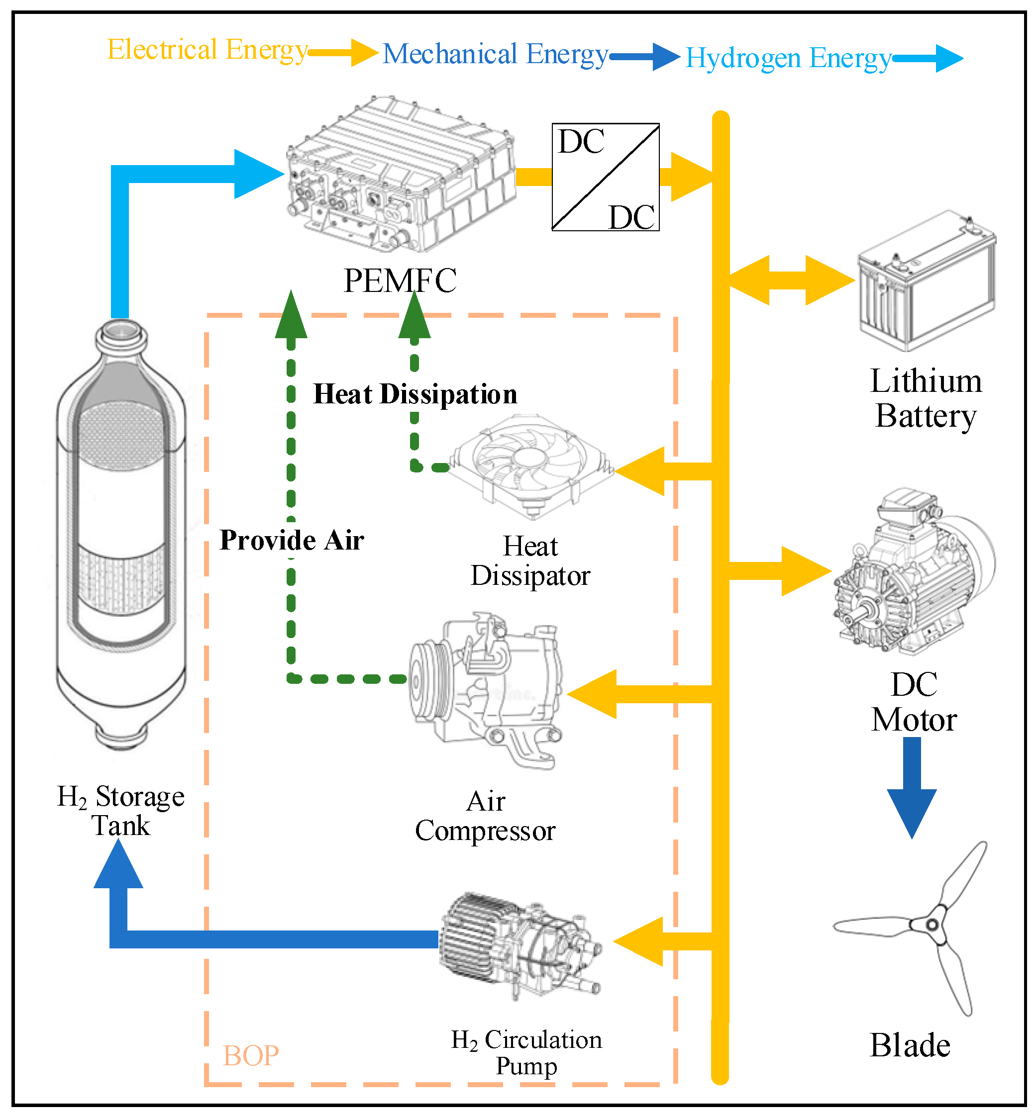
2.1. Hydrogen-Powered Hybrid UAV System Model

2.1.1. Proton Exchange Membrane Fuel Cell

The hydrogen consumption of the proton exchange membrane fuel cell is calculated using Faraday’s law:

$$H^{FC}={\displaystyle \frac{I_{FC}{n}_{FC}}{2F}}$$

(1)

where $H^{FC}$ is the hydrogen consumption rate, $I_{FC}$ is the operating current, and $n_{FC}$ is the number of cells.

The fuel cell reaction rate can be expressed by the current density j:

$$j={\displaystyle \frac{I_{FC}}{A_{cell}}}$$

(2)

where $A_{cell}$ is the reaction area of the fuel cell unit.

The thermal power output of the fuel cell $P_{\mathrm{H}}^{\mathrm{FC}}$ is expressed as follows:

$$P_{\mathrm{H}}^{\mathrm{FC}}=P_{\mathrm{E}}^{\mathrm{FC}}{\displaystyle \frac{{\eta }_{\mathrm{T}}}{{\eta }_{\mathrm{E}}}}$$

(3)

where ${\eta }_T$ is the thermal efficiency of the fuel cell, and ${\eta }_E$ is the electrical efficiency of the fuel cell.

2.1.2. Lithium Battery

The lithium battery operates in a battery pack configuration, and its total power output is expressed as follows:

$$P_{\mathrm{E}}^{\mathrm{B}}=P_{\mathrm{E}}^{\mathrm{b}}\times n_1\times n_2$$

(4)

where $P_{\mathrm{E}}^{\mathrm{B}}$ is the total power output of the battery pack, $P_{\mathrm{E}}^{\mathrm{b}}$ is the power of a single battery cell, $n_1$ and $n_2$ represent the number of rows and columns of the battery cells, respectively.

The current of a battery cell is as follows:

$$I_{\mathrm{b}}={\displaystyle \frac{V_{\mathrm{oc}}-\sqrt{V_{\mathrm{oc}}^2-4R_{\mathrm{b}}{P}_{\mathrm{E}}^{\mathrm{b}}}}{2R_{\mathrm{b}}}}$$

(5)

where the open-circuit voltage V_OC and the internal resistance R_b of the battery cell can both be considered constant values.

The dynamic characteristic of the battery cell, SOC can be expressed as follows:

$${\mathrm{SOC}}_{t+1}={\mathrm{SOC}}_t-{\displaystyle \frac{I_{\mathrm{b},t}}{Q_{\mathrm{B}}}}\Delta T$$

(6)

where t (0 ≤ t ≤ T) is the scheduling time, T is the scheduling period, Q_B is the battery cell capacity, and $I_{\mathrm{b},k}$ is the current, with charging being negative and discharging being positive.

The energy currently stored in the lithium battery is related to the energy stored at the previous time step and the energy charging and discharging between the two-time steps. The upper and lower limits of the stored electrical energy are determined by the device’s capacity, and the charging and discharging power also has upper and lower constraints. Due to the continuity of device operation, the initial storage state of the device at each moment is equal to the final storage state after the previous cruise. When typical cruise data are input, it can be assumed that the storage state at the beginning and end of each cruise is continuous. The energy storage device model can be represented by Equation (7).

$$\begin{array}{l}{E}_{BT,t}=\left\{\begin{array}{ll}{E}_{BT,t-1}\left(1-{\sigma }_{BT}\right)+\left(E_{BT,t-1}^{in}{\eta }_{BT}^{in}-E_{BT,t-1}^{out}/{\eta }_{BT}^{out}\right)\times \Delta t\hfill & t\ne 1\hfill \\ E_{BT,N}\left(1-{\sigma }_{BT}\right)+\left(E_{BT,N}^{in}{\eta }_{BT}^{in}-E_{BT,N}^{out}/{\eta }_{BT}^{out}\right)\times \Delta t\hfill & t=1\hfill \end{array}\right.\\ SO{C}_{BT}^{\min }\le E_{BT,t}\le SO{C}_{BT}^{\max }\\ 0\le E_{BT,t}^{in},E_{BT,t}^{out}\le P{e}_{BT}\end{array}$$

(7)

where $E_{BT,t}$ is the energy storage state of the lithium battery, in kWh; ${\sigma }_{BT}$ is the self-loss coefficient of the lithium battery; $E_{BT,t}^{in}$ and $E_{BT,t}^{out}$ are the charging and discharging power of the lithium battery, in kW, respectively; ${\eta }_{BT}^{in}$ and ${\eta }_{BT}^{out}$ are the charging and discharging efficiencies of the lithium battery, respectively; $SO{C}_{BT}^{\min }$ and $SO{C}_{BT}^{\max }$ are the lower and upper limits of the battery’s storage state, in kWh, respectively; $P{e}_{BT}$ is the maximum electrical power of the lithium battery; and $\Delta t$ is the time interval.

2.1.3. Hydrogen Storage Tank

The hydrogen storage tank uses a high-pressure hydrogen storage tank model (HST) to provide a source of hydrogen for fuel cell power generation. The pressure inside the hydrogen storage tank changes dynamically as hydrogen is released, represented as follows:

$$T{P}_{t+1}^H=T{P}_t^H-z_t{\displaystyle \frac{R{T}_H}{V_H}}{H}_t^{HST}$$

(8)

where $T{P}_t^H$ and $H_t^{HST}$ are the pressure inside the hydrogen storage tank and the hydrogen flow rate at time t, with the flow rate measured in mol/s. $V_H$ is the volume of the hydrogen storage tank, $T_H$ is the operating temperature, R is the universal gas constant, and z_t is the compressibility factor of hydrogen, which can be calculated based on NIST data using the Lemmon equation:

$$z_t(T{P}_t^H)=1+{\displaystyle \sum _{i=1}^9{a}_i}{\left({\displaystyle \frac{T_0}{T_H}}\right)}^{b_i}{(T{P}_t^H)}^{c_i}$$

(9)

where a_i, b_i, and c_i are constants, the values of which can be found in Appendix A 

Table A1. Values of a_i, b_i, and c_i.

i	${\mathit{a}}_{\mathit{i}}$	${\mathit{b}}_{\mathit{i}}$	${\mathit{c}}_{\mathit{i}}$
1	0.0588460	1.325	1.0
2	−0.06136111	1.87	1.0
3	−0.002650473	2.5	2.0
4	0.002731125	2.8	2.0
5	0.001802374	2.938	2.42
6	−0.0012150707	3.14	2.63
7	0.958842 × 10−4	3.37	3.0
8	−0.1109040 × 10−6	3.75	4.0
9	0.1264403 × 10−9	4.0	5.0

. T₀ = 100 K, and R = 8.3145 J/mol·K.

2.1.4. Electric Motor

The system uses a brushless direct current (DC) motor as the main power output, which features low electrical loss, long lifespan, and low maintenance. The equivalent voltage and current of the brushless DC motor are as follows:

$$I_{motor}={\displaystyle \frac{M_{motor}{K}_{V0}{U}_{m0}}{9.55(U_{m0}-I_{m0}{R}_{motor})}}+I_{m0}$$

(10)

$$U_{motor}=R_{motor}{I}_{motor}+{\displaystyle \frac{U_{m0}-I_{m0}{R}_{motor}}{K_{V0}{U}_{m0}}}{N}_{motor}$$

(11)

where $I_{motor}$ is the equivalent current of the motor, $U_{m0}$ is the no-load voltage of the motor, $I_{m0}$ is the no-load current of the motor, $K_{V0}$ is the no-load speed of the motor, $R_{motor}$ is the internal resistance of the motor, $M_{motor}$ is the load torque of the motor, and $N_{mot\mathrm{o}r}$ is the speed of the motor.

The electrical power of the motor is as follows:

$$P_{mot\mathrm{o}r}=U_{motor}\cdot I_{motor}$$

(12)

where $P_{motor}$ represents the rated power of the motor during operation.

2.2. Construction of Uncertainty Model

During the cruise phase of a hydrogen hybrid UAV, suitable wind uncertainty can reflect the basic statistical characteristics of the wind field and meet the requirements for trajectory integration applications, which is crucial for the capacity configuration of long-endurance hydrogen hybrid UAVs. In the local analysis of UAV trajectories that need to maintain intervals, capturing the spatial and temporal correlations of the wind field is key. Typically, in this scenario, assuming that the wind field is steady, homogeneous, and isotropic is reasonable. However, for mid- to long-range trajectory prediction that supports Air Traffic Control (ATC) and Decision Support Tools (DSTs), the model needs to reflect the non-stationarity, non-homogeneity, weather-dependency, and potential non-Gaussian characteristics of the wind field. This model satisfies the requirements for long-endurance hydrogen hybrid UAV capacity configuration.

A convenient method for modeling wind uncertainty is to effectively utilize a large amount of historical RUC (Rapid Update Cycle) data, which are provided by the National Weather Service’s numerical weather prediction system [20]. However, since RUC data are only valid at discrete network points and specific time points, appropriate interpolation schemes are required to obtain wind uncertainty samples for general locations and times while preserving the spatial and temporal correlations of wind error fields.

Wind uncertainty samples for a general location and forecast time period are obtained by weighted summation of historical RUC wind errors from nearby locations. These neighboring points are selected within the spatial range of the current location. For each location, historical RUC wind error data are derived from delayed RUC forecasts during the same time period in the same season under similar conditions. The forecast time interval is within the temporal correlation time range of the specified prediction time. The weight selection in the model is inversely proportional to the square of the relative distance and the absolute value of the forecast time interval difference. Additionally, the model includes two purely random correction terms to account for other sources of uncertainty.

$$\Delta W_{G,j}(r,\tau )=-{\displaystyle \sum _k{L}_k(\tau )}{\displaystyle \sum _i{C}_i(r_i)}[\Delta W_{G,j}^{RUC}(r_i,{\tau }_k)+{\epsilon }_{G,j}^m(r_i,{\tau }_k)]+{\epsilon }_{G,j}^r$$

(13)

where j = 1, …, N_s represents the sample number of wind uncertainty, $\Delta W_{G,j}(r,\tau )$ represents the position vector denoted as r, and the predicted wind uncertainty at the forecast lead time τ is represented. $\Delta W_{G,j}^{RUC}$ represents the wind components provided by RUC. ${\epsilon }_{G,j}^m(r,{\tau }_k)$ represents the pure random variable where the position vector is r, the sample index of wind uncertainty is j, and the forecast lead time is τ_k. ${\epsilon }_{G,j}^r$ represents the pure random variable where the position vector is r and the sample index of wind uncertainty is j. r and r_i represent the position vector and the position vector at grid point index i. τ and τ_k represent the forecast lead time, where τ_k = 0, 1, …, 9. m represents the mass of the aircraft. And C_i(r) and L_k(τ) are as follows:

$$C_i(r)={\displaystyle \frac{{\left|r-r_i\right|}^{-p}}{{\displaystyle \sum _{k=1}^{N_R}{\left|r-r_k\right|}^{-p}}}},L_k(\tau )={\displaystyle \prod _{k\ne j}^{N_t}\left(\frac{\tau -{\tau }_k}{{\tau }_j-{\tau }_k}\right)}$$

(14)

In the equation, C_i(r) and L_k(τ) both represent weights, where C_i(r) is related to position, and L_k(τ) is related to the forecast lead time.

Due to the variations in different geographical regions and between different predictions in each RUC forecast, the resulting model is naturally non-stationary, non-homogeneous, non-Gaussian, and weather-dependent. Additionally, uncertainties arising from initial measurements and the determination of the nominal wind field can also be appropriately incorporated into the model.

$$-\Delta W_G(r,t+\tau |t)=\Delta W_G^{RUC}(r,t+\tau |t)+e_G^m(r,t+\tau )+e_G^n(r,t+\tau |t)$$

(15)

In the equation, $-\Delta W_G(r,t+\tau |t)$ represents the wind uncertainty prediction at the position vector r and forecast lead time t + τ, based on the value at time t; $\Delta W_G^{RUC}(r,t+\tau |t)$ represents the time-lagged RUC data error at position vector r and forecast lead time τ, based on the value at time t; $e_G^m(r,t+\tau )$ and $e_G^n(r,t+\tau |t)$ represent the initial measurement error and nominal wind error, respectively.

Equation (15) shows how the initial measurement inputs of the RUC model introduce uncertainty. The basis for the measurements is the relationship between certain physical properties of the wind field and the wind speed and direction. Thus, the measurement errors can be divided into calibration errors of the equipment and errors caused by uncertainties in the underlying physical processes. While further research is needed, it can be assumed that the latter follows a pattern similar to wind errors. Therefore, a pure random term is added to the model to account for the correlated part of the measurement error, while another pure random term is added outside the weighted summation to represent the measurement calibration error.

In contrast, the uncertainty introduced during the nominal wind field determination depends on the specific interpolation or approximation method used. When interpolation is performed, the error is zero at the RUC network points, which are spaced 20 km apart in the horizontal direction and 25 hPa apart in the vertical direction. Thus, the horizontal spatial scale of the error is approximately 40 km. This is significantly smaller than the spatial correlation of wind errors and is therefore considered a pure random term. Additionally, the residuals of the weighted summation model are random, as the summation already accounts for the spatial and temporal correlations. Therefore, in Equation (13), ${\epsilon }_G^m$ represents the pure random corrections for measurement calibration errors, nominal wind field determination errors, and model residuals.

When constructing the above wind uncertainty model, it is assumed that the measurement errors, nominal wind field determination errors, and RUC system prediction errors are independent of each other. The following additional assumptions are also made:

The wind uncertainty components along the three vertical directions are uncorrelated. Therefore, the corresponding 3 × 3 correlation matrix is a diagonal matrix, and the components along the three directions can be analyzed separately. It should be noted that the correlation of different wind quantities is influenced by the choice of coordinate system. This patent adopts the wind directions along the three vertical axes.

Compared to the horizontal components, the vertical wind component Wh is relatively small and is often neglected. However, the actual vertical wind may not be zero, and its presence could affect the accuracy of the predicted trajectory.

In meteorological models, commonly used interpolation methods include linear interpolation, bilinear interpolation, spline interpolation, and inverse distance weighting (IDW), among others. For wind fields involving wind speed and direction, IDW is relatively common, but it is not well suited for capturing complex nonlinear variations. Therefore, a combination of spline interpolation and IDW is adopted.

Inverse Distance Weighting (IDW) is an interpolation method based on Tobler’s First Law of Geography. It uses the distance between the point to be estimated and the measured values as a weighting factor, and infers the attributes of the unknown point based on the known values. The expression is as follows:

$$Z(x)={\displaystyle \sum _{i=1}^n{W}_i}Z(x_i)$$

(16)

where Z(x) represents the estimated value at the point to be interpolated, Z(x_i) represents the value at the i-th interpolation point, n is the number of interpolation points involved, and W_i represents the weight of the i-th interpolation point. The calculation of the weight W_i is as follows:

$$W_i={\displaystyle \frac{d_{(x,x_i)}^{-a}}{{\displaystyle \sum _{i=1}^n{d}_{(x,x_i)}^{-a}}}}$$

(17)

where a is the distance exponent, $d_{(x,x_i)}$ is the distance from the i-th interpolation point x_i to the point to be estimated x, and the weight W_i decreases as the distance increases. Additionally, the larger the distance exponent a, the greater the weight assigned to interpolation points closer to the target point, making the interpolated value closer to the value of the nearest interpolation point. Conversely, a smaller a result in the interpolated value is closer to the average of the surrounding interpolation points.

Spline interpolation simulates the shape of a given curve by inserting spline curves between known points, resulting in a smoother and more accurate outcome.

Let the interpolation be performed on the interval [a, b], where a = x₁ < x₂ < ⋯ < x_n = b, and each interpolation point have a corresponding function value, denoted as F(x_i) = y_i (i = 1, 2, …, n). If the function F(x) is a polynomial of degree at most 3 on the interval [a, b], and F(x) has a second derivative on the interval [a, b], then F(x) is called a cubic spline interpolation function.

Specifically, F(x) exists as a cubic polynomial on each subinterval [x_i, x_i + 1], which can be expressed as F_i(x) = a_ix³ + b_ix² + c_ix + d_i, where F(x_i) = y_i, F(x_i − 0) = F(x_i + 0), F′(x_i − 0) = F′(x_i + 0), F″(x_i − 0) = F″(x_i + 0), (i = 1, 2, …, n−1).

By combining the two methods, a multi-scale interpolation approach is adopted. Since the data scale range provided by the RUC model is too large, with the minimum spatial resolution being 13 km, it is not suitable for long-endurance hydrogen hybrid UAVs. First, IDW is used to reduce the data to a 1 km scale, and then cubic spline interpolation is applied to further reduce the IDW-processed data to a 5 m horizontal resolution, ensuring the capture of small variations in airflow.

3. Two-Stage Stochastic Optimization Problem

In actual flight scenarios, wind speed and wind direction are characterized by randomness, volatility, and intermittency. Deterministic models for optimizing the system’s total cost fail to account for these uncertainties, leading to a significant deviation between the optimization results and the actual situation. Therefore, a two-stage stochastic programming model is developed to optimize the capacity configuration of hydrogen hybrid UAVs considering uncertainty.

This study proposes a two-stage stochastic programming model that uses the particle swarm optimization (PSO) algorithm to optimize the first-stage device capacity. The second stage uses random wind speed and wind direction scenarios generated by the Monte Carlo method, combining the optimal device capacity from the first stage to obtain the expected optimal cost of the system under different scenarios. This expected cost serves as the fitness function for the PSO algorithm, continuously evolving the first-stage optimization process. It can be understood as taking the UAV’s flight power demand as input, and after considering the uncertainty of the wind field, along with balance constraints, capacity constraints, and energy storage constraints, deriving the expected optimal cost of the system under different scenarios. Then, the particle swarm optimization algorithm is used to optimize the system, ultimately determining the optimal equipment capacity to meet various flight scenarios. CPLEX typically uses branch-and-bound and cutting-plane methods to solve MILP models, incorporating preprocessing and heuristic methods. Therefore, the CPLEX solver can be used to solve the second-stage MILP problem. The specific process is shown in Figure 2.

The process is based on solving the MILP problem and the PSO algorithm, using Monte Carlo simulation to generate random scenarios for the system, and accounting for uncertainty in the system. The main steps include particle swarm generation, fitness calculation, particle position update, particle velocity update, boundary check, and termination condition check. The specific computational steps are as follows:

• Step 1: Initial Particle Swarm Generation:

Define the space range within which the particles can move. Within this range, randomly generate the position vector and velocity vector for each particle.

• Step 2: Fitness Calculation:

For each individual in the particle swarm, substitute it into each scenario generated by Monte Carlo simulation to obtain the expected value for each scenario, i.e., the fitness of the individual. In cases of no solution or failed solution, a large value can be added to the fitness function to lower the fitness of that individual, further screening the particles.

• Step 3: Update Global Best Particle and Individual Best Particle:

Based on the fitness function values, select the particle with the best fitness among the current individuals, as well as the global best particle.

• Step 4: Boundary Check:

Verify the updated particle positions and velocities, and if any particle exceeds the boundary, regenerate its position and velocity randomly.

• Step 5: Repeat Steps 2–4 until the iteration conditions are met, exit the loop, and obtain the optimal solution.

In addition, PSO includes the number of particles, N, maximum number of iterations, Max_iteration, dimensionality, dim, lower boundary of the search space, I_b, and upper boundary of the search space, u_b. The core of the PSO algorithm is to simulate the movement of multiple particles within the search space, where each particle represents a potential solution. The selection of the number of particles needs to balance performance and computation time. The maximum number of iterations refers to the maximum number of updates for the particles’ velocity and position. The lower and upper boundaries of the search space define the lower and upper limits of the decision variables.

Considering that the hydrogen hybrid UAV is greatly affected by wind speed and wind direction, and that fluctuations in climate conditions are often random and difficult to predict, the capacity configuration results obtained through deterministic models for optimizing the system’s total cost may be inaccurate. This paper proposes a two-stage stochastic programming method to study the optimization problem of capacity configuration for hydrogen hybrid UAVs.

First, system constraints are established, primarily including energy balance constraints, capacity constraints, and energy storage constraints.

3.1. Energy Balance Constraint

In the hydrogen hybrid UAV energy system, the primary focus is on the electrical load demand. During system operation, the electrical energy obtained by the system should be greater than or equal to the energy consumption. The devices that generate electrical energy in the system include hydrogen fuel cells and lithium batteries. The devices that consume electrical energy include DC motors, fans, communication equipment, and lithium batteries. The energy balance is represented by the following equation:

$$E_{FC}+E_{BT}^{out}\ge E_M+E_F+E_{CD}+E_{BT}^{in}$$

(18)

where E_FC represents the electrical energy provided by the hydrogen fuel cell, $E_{BT}^{out}$ represents the electrical energy output by the lithium battery, E_M represents the electrical energy consumed by the DC motor, E_F represents the electrical energy consumed by the fan, E_CD represents the electrical energy consumed by the communication equipment, and $E_{BT}^{in}$ represents the electrical energy input to the lithium battery.

Capacity constraint: For the hydrogen hybrid UAV system, the output power of each device should not exceed its designed capacity. Furthermore, for the hydrogen fuel cell, its minimum operating power should not be lower than 30% of its capacity to avoid operating under excessively low load. Therefore, the capacity constraints for the hydrogen fuel cell and fan are as follows:

$$Y_{FC,t}\times 0.3Ca{p}_{FC}\le E_{FC}\le Y_{FC,t}\times Ca{p}_{FC}$$

(19)

$$0\le E_F\le Y_{F,t}\times Ca{p}_F$$

(20)

In the equation, $Y_{FC,t}$ represents the Boolean variable used to determine whether the hydrogen fuel cell is operating, with a value of 0 or 1; $Ca{p}_{FC}$ represents the maximum output power of the hydrogen fuel cell; $Y_{F,t}$ represents the Boolean variable used to determine whether the fan is operating, with a value of 0 or 1; $Ca{p}_F$ represents the maximum output power of the fan.

3.2. Energy Storage Constraint

For the lithium battery, which serves as the energy storage device, the following assumptions and constraints apply: (1) Before the hydrogen hybrid UAV takes off, the lithium battery has already stored a certain amount of electrical energy. (2) Due to the continuity of multiple flight missions by the hydrogen hybrid UAV, when the hydrogen fuel supply is sufficient, no recharging of the lithium battery is considered. Therefore, the lithium battery’s energy level at the end of the previous flight is assumed to be the same as the starting energy level for the next flight. (3) The storage and withdrawal of energy from the lithium battery do not occur simultaneously and should not exceed the maximum storage and withdrawal power of the battery. (4) The stored energy in the lithium battery should remain within 20% to 80% of its designed capacity.

Therefore, for the lithium battery, the following constraints apply:

$$SO{C}_0=SO{C}_{360}$$

(21)

$$0\le SO{C}_{in}\le Y_{SOC,t}\times P_{in,\max }$$

(22)

$$0\le SO{C}_{out}\le (1-Y_{SOC,t})\times P_{out,\max }$$

(23)

$$0.2Ca{p}_{soc}\le SO{C}_t\le 0.8Ca{p}_{soc}$$

(24)

In the equation, $Y_{SOC,t}$ represents the Boolean variable used to determine whether the lithium battery is charging or discharging, with a value of 0 or 1; $P_{in,\max }$ represents the maximum charging power of the lithium battery; $P_{out,\max }$ represents the maximum discharging power of the lithium battery; $Ca{p}_{soc}$ represents the capacity of the lithium battery.

For the hydrogen storage tank, which serves as the hydrogen energy storage device, the following assumptions and constraints apply:

(1)

Before the hydrogen hybrid UAV takes off, the hydrogen storage tank has already stored a certain amount of hydrogen energy.

(2)

Due to the continuity of multiple flight missions by the hydrogen hybrid UAV, when the hydrogen fuel is at no less than 20% of its maximum capacity, refueling is not required. Therefore, the amount of hydrogen in the storage tank at the end of the previous flight is assumed to be the same as the starting amount for the next flight.

(3)

The storage and withdrawal of hydrogen from the tank do not occur simultaneously. Since the refueling process does not affect the capacity configuration of the hydrogen hybrid UAV, the focus is more on the withdrawal rate, which should not exceed the maximum withdrawal power of the hydrogen storage tank.

Therefore, for the hydrogen storage tank, the following constraints apply:

$$T{P}_0=\left\{\begin{array}{l}T{P}_{\max },if T{P}_{360}<0.2T{P}_{\max }\\ T{P}_{360},else\end{array}\right.$$

(25)

$$0\le T{P}_{out}\le (1-Y_{TP,t})\times H_{out,\max }$$

(26)

In the equation, $Y_{TP,t}$ represents the Boolean variable used to determine whether the hydrogen storage tank is releasing hydrogen, with a value of 0 or 1; $H_{out,\max }$ represents the maximum hydrogen release power of the hydrogen storage tank.

A stochastic programming model is constructed for the capacity configuration of the hydrogen hybrid UAV.

The variables in the stochastic model for the capacity configuration of the hydrogen hybrid UAV include design variables, which refer to the capacity of the equipment, and operational variables, which refer to the variables during the operation of the hydrogen hybrid UAV. Based on these variables, an MILP problem is constructed:

$$\begin{array}{c}\underset{d,x_t,y_t}{\min }f(d,x_t,y_t)\\ \begin{array}{c}\begin{array}{c}\mathrm{s}.\mathrm{t}.{\displaystyle }{\psi }^{dc}(d)\le 0\end{array}\\ {\phi }^{oc}(d,x_t,y_t)=0\\ {\psi }^{oc}(d,x_t,y_t)\le 0\end{array}\\ d\in {\Re }^1,x_t\in {\Re }^n,y_t\in {\left\{0,1\right\}}^n\end{array}$$

(27)

where d represents the continuous decision variables determined during the design process; x_t and y_t represent the continuous variables and 0-1 binary variables involved in the operation process, respectively, existing within each time interval during the project lifecycle; f is the objective function, i.e., the total cost of the system over its entire lifecycle; ${\psi }^{dc}$ represents inequality constraints in the design process, which are related only to the design variables d; ${\phi }^{oc}$ and ${\psi }^{oc}$ represent equality and inequality constraints during the operational process, which are related to the operational variables x_t, y_t, and d. ${\Re }^1$ and ${\Re }^n$ represent the feasible regions of the respective continuous variables determined, and the feasible region of the continuous variables involved in the operation process; n represents the dimensionality, i.e., the number of 0-1-type variables. When considering the impact of uncertain parameters on the optimization problem, the problem above becomes a typical two-stage resource problem. For a deterministic MILP problem, the design variables and operational variables can be determined simultaneously and optimally. However, for a stochastic optimization problem, the design variables, which are independent of uncertain parameters, can be determined first (here-and-now), while the operational variables must wait until all random parameters have been realized in order to determine the optimal solution (wait-and-see). In other words, the two types of variables need to be determined at different stages of the optimization process.

Therefore, when both the design variables and operational variables need to be optimized simultaneously to minimize the total lifecycle cost of the system, this study adopts a two-stage stochastic programming approach. All design variables, i.e., the capacities of all devices, are classified as first-stage variables; all operational variables are classified as second-stage variables. Combining the MILP problem above, this two-stage stochastic programming problem can be expressed in the following form:

$$\begin{array}{ll}\left(\mathrm{First-stage}\right):\hfill & \begin{array}{l}\min ({\omega }_1{C}_{\mathit{short}}+{\omega }_2{C}_{\mathit{long}})\\ =\min [{\omega }_1(k_1{C}_f+k_2{C}_m)+{\omega }_2(k_3{C}_e+k_4{C}_l)]\\ =\min [{\omega }_1{k}_1{C}_f+({\omega }_1{k}_2{C}_m+{\omega }_2{k}_3{C}_e+{\omega }_2{k}_4{C}_l)]\\ =\underset{d}{\min }E[f_s(d,\mathit{\xi })]+f_d(d)\end{array}\\ & \mathrm{s.t.}{\psi }^{dc}(d)\le 0\\ & \hspace{1em}\hspace{1em}d\in \{0,1\}\\ \left(\mathrm{Second-stage}\right):\hfill & f_s(d,\mathit{\xi })=\underset{x_t,y_t}{\min }{f}_s(d,x_t,y_t,\mathit{\xi })\\ & \begin{array}{ll} \mathrm{s.t.}& {\phi }^{oc}(d,x_t,y_t,\mathit{\xi })=0\\ & {\psi }^{oc}(d,x_t,y_t,\mathit{\xi })\le 0\\ & x_t\in {\mathfrak{R}}^n,y_t\in \{0,1{\}}^n\end{array}\end{array}$$

(28)

The objective function is represented by two parts: $f_d$ is the deterministic part of the objective function, which corresponds to the investment cost $C_{inv}$ of the selected equipment capacity. The stochastic part is represented by the expectation of $f_s$, which represents the cost related to the uncertain parameters, including the operation and maintenance costs $C_{OM}$ and the cost of purchasing resources $C_{tari}$. ξ represents the uncertain parameters, including wind speed, wind direction, and load size.

The comprehensive evaluation metric with multiple time scales primarily refers to the coupling between short-term decisions and long-term planning, where short-term decisions focus on immediate costs, and long-term planning focuses on long-term costs.

Short-term decisions emphasize immediate benefits. In the case of the hydrogen hybrid UAV, short-term costs include hydrogen fuel consumption costs and regular maintenance costs.

Long-term planning focuses on the sustainability of the system. For the hydrogen hybrid UAV, long-term costs include the initial investment in equipment and the service life of the equipment.

The corresponding objective function is constructed using a weighted sum:

$$\min J={\omega }_1{C}_{\mathit{short}}+{\omega }_2{C}_{long}$$

(29)

where J is the objective value of the comprehensive optimization; C_short is the short-term cost, including fuel consumption and maintenance costs; C_long is the long-term cost, including equipment investment and the amortized service life; ω₁ and ω₂ are the weight coefficients that balance the relative importance of short-term and long-term objectives.

Short-term cost:

$$C_{short}=k_1{C}_f+k_2{C}_m$$

(30)

where C_f represents the hydrogen fuel consumption cost, C_m represents the regular maintenance cost, and k₁, k₂ are the weight coefficients.

$$C_f=P_f\cdot Q_f$$

(31)

where P_f represents the unit price of hydrogen fuel, in ¥/L, Q_f represents the hydrogen consumption of the fuel cell for a single flight, in liters L, $Q_f=f(I_{FC},t)$, I_FC represents the fuel cell operating current, and t represents the duration of a single flight.

$$C_m={\displaystyle \frac{1}{N_m}}{\displaystyle \sum _{n=1}^{N_{mn}}(K_n{C}_n)}$$

(32)

where N_m represents the number of flights within the regular maintenance cycle, N_mn represents the number of devices on the hydrogen hybrid UAV that require regular maintenance, K_n is the equipment maintenance cost coefficient, and C_n represents the equipment parameters. Taking the lithium battery as an example, K_n represents the unit price during the maintenance or inspection process, in CNY/kWh, and C_n represents the capacity of the lithium battery, in kWh.

Long-term cost:

$$C_{long}=k_3{C}_e+k_4{C}_l$$

(33)

where C_e represents the one-time investment cost of the equipment, C_l represents the amortized cost of the service life, and k₃, k₄ are the weight coefficients.

$$C_e={\displaystyle \sum _{\mathrm{n}=1}^{N_e}{P}_n}$$

(34)

where N_e represents the number of devices that require a one-time investment, and P_n represents the cost of the equipment.

$$C_l={\displaystyle \sum _{n=1}^{N_l}\frac{P_n-P_{n,ev}}{N_u}}$$

(35)

where N_l represents the number of devices that require amortization of their service life, P_n represents the cost of the equipment, P_n,ev represents the residual value, i.e., the remaining value of the equipment at the end of its service life, and N_u represents the service life (here measured in terms of usage cycles).

4. Results

Based on the proposed wind uncertainty model and RUC data, a set of possible wind speed and wind direction datasets is calculated, as shown in Appendix A 

Table A2. The dataset of wind speed and wind direction obtained from the wind uncertainty model.

Time (min)	Wind Speed (m/s)	Wind Speed Uncertainty (±m/s)	Wind Direction (°)
0	3.5	±0.3	45
10	3.2	±0.3	42
20	3.8	±0.4	47
30	3.6	±0.4	50
40	4	±0.3	48
50	3.9	±0.5	53
60	4.3	±0.5	57
70	4.5	±0.4	55
80	4.1	±0.5	59
90	4.6	±0.5	63
100	4.8	±0.5	60
110	4.5	±0.5	65
120	5	±0.4	68
130	4.7	±0.6	66
140	5.2	±0.6	70
150	5.4	±0.6	72
160	5.1	±0.6	75
170	5.3	±0.7	73
180	5.6	±0.7	77
190	5.8	±0.6	75
200	5.4	±0.7	78
210	5.9	±0.7	82
220	6.1	±0.7	80
230	6	±0.8	85
240	6.2	±0.8	83
250	6.3	±0.8	87
260	6.5	±0.5	89
270	6.6	±0.8	86
280	6.4	±0.9	91
290	6.8	±0.3	88
300	6.9	±0.8	92
310	6.7	±0.4	90
320	7	±0.9	95
330	6.8	±1.2	93
340	7.2	±1.0	98
350	7.1	±1.0	100
360	7.3	±0.3	97

.

Based on the proportion of each device in Figure 3, Figure 4 and Figure 5, the parameter settings for the objective function are shown in

Table 1. Objective function parameter settings.

Parameter	Value	Parameter	Value	Parameter	Value
ω1	0.4	K1	0.2	P1	500
ω2	0.6	K2	0.4	P2	2000
k1	0.1	K3	0.1	P3	300
k2	0.9	K4	0.2	P4	100
k3	0.5	C1	500	P1,ev	50
k4	0.5	C2	800	P2,ev	250
Pf	0.0025	C3	20	P3,ev	50
Nm	50	C4	400	P4,ev	20
Nmn	4	Ne	4	Nu	2000

.

First, Monte Carlo sampling is used to sample the wind uncertainty model, obtaining deterministic models and corresponding optimal device capacities for multiple scenarios, as well as the expected optimal cost under different scenarios. The expected optimal cost is used as the fitness function for the particle swarm optimization algorithm, which continuously optimizes the first-stage optimization process. The MILP problem in the second stage is solved using the CPLEX solver in MATLAB 2024a. The particle swarm parameters are listed in

Table 2. Parameter settings of PSO algorithm.

Parameter	Value
N	50
Max_iteration	1000
dim	4
lb	[0, 0, 0, 0]
ub	[5, 10, 100, 12]

. The convergence results of the particle swarm optimization are shown in Figure 6.

Additionally, a sensitivity analysis on the number of particles NNN was conducted by testing with values of 30, 50, and 100, and the results are shown in Figure 7. As can be seen from the figure, the convergence result is better when the number of particles is set to 50.

The capacity configuration results for the hydrogen-powered hybrid UAV, derived from the objective function parameter settings shown in Table 2, are presented in

Table 3. Capacity configuration results.

Device	Parameter
Fuel cell (Kw)	Pmax = 3.367, Pr = 2.525
Lithium battery (kWh)	Battery Capacity 7.694
Cooling system (W)	Thermal Power 53.128
Hydrogen storage tank (L)	V = 9.328

.

From

Table 4. Comparison table of PSO and GA algorithms.

Indicators	PSO	GA
The optimal lifecycle cost (CNY ten thousand)	30.15	31.20
Number of iterations	143	256
Computation time (s)	63	102
Post-iteration error (%)	0.5	1.2
Number of feasible solutions (%)	98	92

, particle swarm optimization (PSO) outperforms the genetic algorithm (GA) in terms of optimization speed, computation time, and solution quality. Although the GA has advantages in global search capability, PSO is better suited for scenarios requiring efficient optimization, particularly in capacity configuration problems, due to its lower computational complexity and faster convergence rate. PSO demonstrates better performance, especially in real-time capacity configuration and lifecycle cost minimization for unmanned aerial vehicles.

5. Conclusions

This research proposes a capacity configuration optimization model for hydrogen UAVs based on two-stage stochastic optimization, aiming to account for the impact of uncertain factors such as wind speed and wind direction. The model integrates both short-term and long-term costs of the UAV, providing an optimal capacity configuration for hydrogen hybrid UAVs. By introducing a combination of PSO algorithm and Monte Carlo simulation, the model overcomes the limitations of existing deterministic models that cannot effectively address uncertainty. The model incorporates multiple key factors, including energy balance constraints, equipment capacity constraints, and energy storage constraints, ensuring the feasibility and efficiency of the optimization results in actual flight scenarios. The main contributions and conclusions are as follows:

(1)

The two-stage stochastic optimization method proposed in this paper effectively addresses the impact of uncertain factors such as wind speed and wind direction. In the first stage, PSO is used to optimize the capacity configuration of the equipment, while the second stage evaluates the expected optimal cost under different scenarios by solving the MILP problem, ultimately achieving the system’s full lifecycle optimization.

(2)

This paper constructs a comprehensive evaluation metric that includes both short-term and long-term costs. The short-term costs focus on hydrogen consumption and regular maintenance expenses, while the long-term costs consider equipment investment and amortization of service life. By using a weighted sum, the short-term and long-term objectives are balanced, ensuring that the system meets the immediate operational needs while maintaining long-term sustainability.

(3)

To address the uncertainty of wind speed and wind direction, the Monte Carlo method is used to generate random scenarios for these variables. By combining this with the PSO algorithm, the system configuration is continuously optimized. Through iterative optimization, the PSO algorithm effectively finds the optimal solution, thereby improving the overall system performance.

(4)

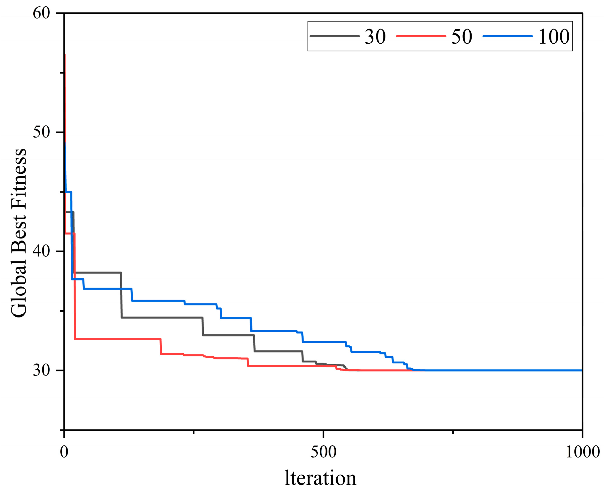
A sensitivity analysis of the number of particles in the PSO algorithm was conducted, and the results showed that the optimization effect was best when the number of particles was set to 50. This provides valuable guidance for future optimization algorithm configurations, ensuring both computational efficiency and convergence.

Although the optimization method proposed in this paper has shown good results under various uncertain scenarios, there is still room for further improvement. First, the current model primarily considers the uncertainties of wind speed and wind direction. Future research could introduce additional environmental factors, such as temperature changes, weather fluctuations, and power demand, to further enhance the model’s applicability and accuracy. Moreover, with the continuous advancement of technology, the application scenarios of hydrogen hybrid UAVs will become more complex. Future studies could explore dynamic optimization methods based on real-time data, which involve monitoring various flight parameters in real time and adjusting flight strategies accordingly to improve operational efficiency.

Additionally, the optimization goal in this paper focuses on cost minimization. However, in practical applications, multiple objectives may need to be balanced, such as environmental impact, operational safety, and others. Future research could consider incorporating these factors into the optimization framework and conduct multi-objective optimization to achieve more comprehensive performance improvements. Furthermore, with the rapid development of artificial intelligence and machine learning technologies, future research could attempt to combine these advanced technologies with traditional optimization algorithms. Methods like deep learning could be used to enhance the accuracy and intelligence of the optimization process.

Regarding the optimization algorithm, although the PSO algorithm has shown good performance, it also has certain limitations. Future studies could attempt to combine PSO with other optimization methods, such as genetic algorithms or ant colony optimization, or even develop new hybrid optimization algorithms to improve solution efficiency and algorithm robustness. Additionally, with the advancement of computational power, the scale of the problem can be expanded, allowing for the resolution of more complex optimization problems.

References

1. Cho, H.; Mago, P.J.; Luck, R.; Chamra, L.M. Evaluation of CCHP systems performance based on operational cost, primary energy consumption, and carbon dioxide emission by utilizing an optimal operation scheme. Appl. Energy 2009, 86, 2540–2549. [Google Scholar] [CrossRef]
2. Gu, W.; Wu, Z.; Yuan, X. Microgrid economic optimal operation of the combined heat and power system with renewable energy. In Proceedings of the IEEE PES General Meeting, Minneapolis, MN, USA, 25–29 July 2010; pp. 1–6. [Google Scholar]
3. Liu, C.; Wang, C.; Yin, Y.; Yang, P.; Jiang, H. Bi-level dispatch and control strategy based on model predictive control for community integrated energy system considering dynamic response performance. Appl. Energy 2022, 310, 118641. [Google Scholar] [CrossRef]
4. Zhang, Z.; Wang, C.; Lv, H.; Liu, F.; Sheng, H.; Yang, M. Day-ahead optimal dispatch for integrated energy system considering power-to-gas and dynamic pipeline networks. IEEE Trans. Ind. Appl. 2021, 57, 3317–3328. [Google Scholar]
5. Li, Y.; Zhang, J.; Wu, X.; Shen, J.; Lee, K.Y. Optimal design of combined cooling, heating and power multi-energy system based on load tracking performance evaluation of adjustable equipment. Appl. Therm. Eng. 2022, 211, 118423. [Google Scholar]
6. Rafiei, M.; Ricardez-Sandoval, L.A. New frontiers, challenges, and opportunities in integration of design and control for enterprise-wide sustainability. Comput. Chem. Eng. 2020, 132, 106610. [Google Scholar]
7. Lenhoff, A.M.; Morari, M. Design of resilient processing plants—I Process design under consideration of dynamic aspects. Chem. Eng. Sci. 1982, 37, 245–258. [Google Scholar]
8. Seferlis, P.; Grievink, J. Process design and control structure screening based on economic and static controllability criteria. Comput. Chem. Eng. 2001, 25, 177–188. [Google Scholar]
9. Papadopoulos, A.I.; Seferlis, P.; Linke, P. A framework for the integration of solvent and process design with controllability assessment. Chem. Eng. Sci. 2017, 159, 154–176. [Google Scholar]
10. Yu, W.; Li, K.; Li, S.; Ma, X.; Zhang, C. A bi-level scheduling strategy for integrated energy systems considering integrated demand response and energy storage co-optimization. J. Energy Storage 2023, 66, 107508. [Google Scholar]
11. Shen, F.; Zhao, L.; Wang, M.; Du, W.; Qian, F. Data-driven adaptive robust optimization for energy systems in ethylene plant under demand uncertainty. Appl. Energy 2022, 307, 118148. [Google Scholar] [CrossRef]
12. Yu, J.; Ryu, J.H.; Lee, I.B. A stochastic optimization approach to the design and operation planning of a hybrid renewable energy system. Appl. Energy 2019, 247, 212–220. [Google Scholar] [CrossRef]
13. Ioannou, A.; Fuzuli, G.; Brennan, F.; Yudha, S.W.; Angus, A. Multi-stage stochastic optimization framework for power generation system planning integrating hybrid uncertainty modelling. Energy Econ. 2019, 80, 760–776. [Google Scholar] [CrossRef]
14. Gong, A.; MacNeill, R.; Verstraete, D.; Palmer, J.L. Analysis of a Fuel-Cell/Battery/Supercapacitor Hybrid Propulsion System for a UAV using a Hardware-in-the-Loop Flight Simulator. In Proceedings of the 2018 AIAA/IEEE Electric Aircraft Technologies Symposium. Cincinnati, Ohio: American Institute of Aeronautics and Astronautics, Cincinnati, OH, USA, 12–14 July 2018. [Google Scholar]
15. Zhang, X.; Liu, L.; Dai, Y.; Shen, H. Design and Experiment of Fuel Cell UAV Power System. J. Aeronaut. 2018, 39, 162–171. [Google Scholar]
16. Zhang, X.; Liu, L.; Dai, Y. Energy Management and Flight State Coupling of Fuel Cell UAVs. J. Aeronaut. 2019, 40, 92–108. [Google Scholar]
17. Fang, M.; Sun, X.; Huang, R.; Qian, G.; Geng, H.; Wen, G.; Xu, C.; Xu, C.; Liu, L. Automatic Detection of Power Pole Towers for High-Resolution Satellite Remote Sensing. Aerosp. Return Remote Sens. 2021, 42, 118–126. [Google Scholar]
18. Gong, A.; Palmer, J.L.; Brian, G.; Harvey, J.R.; Verstraete, D. Performance of a hybrid, fuel-cell-based power system during simulated small unmanned aircraft missions. Int. J. Hydrogen Energy 2016, 41, 11418–11426. [Google Scholar] [CrossRef]
19. Min, Z.; Lei, T.; Wang, Y.; Zhang, X.; Zhang, X. The Evaluation and Optimization of Power Architecture of Distributed Electrical Propulsion Fuel-cell UAV. In Proceedings of the IECON 2020 The 46th Annual Conference of the IEEE Industrial Electronics Society, Singapore, 18–21 October 2020; pp. 2376–2381. [Google Scholar]
20. Zheng, Q.; Zhao, Y. Modeling wind uncertainties for stochastic trajectory synthesis. In Proceedings of the 11th AIAA Aviation Technology, Integration, and Operations (ATIO) Conference, including the AIAA Balloon Systems Conference and 19th AIAA Lighter-Than, Virginia Beach, VA, USA, 20–22 September 2011; p. 6858. [Google Scholar]
Figure 1. Hydrogen hybrid UAV energy system structure diagram.
Algorithms 18 00196 g001
Figure 2. Two-stage stochastic optimization process.
Algorithms 18 00196 g002
Figure 3. Percentage of equipment maintenance costs.
Algorithms 18 00196 g003
Figure 4. Proportion of unit price per capacity.
Algorithms 18 00196 g004
Figure 5. Salvage value of the equipment at the end of its useful life.
Algorithms 18 00196 g005
Figure 6. Convergence result graph.
Algorithms 18 00196 g006
Figure 7. Sensitivity analysis of the number of particles.
Algorithms 18 00196 g007