Article

The Prediction Performance Analysis of the Lasso Model with Convex Non-Convex Sparse Regularization

School of Information and Mathematics, Yangtze University, Jingzhou 434020, China
*
Author to whom correspondence should be addressed.
Algorithms 2025, 18(4), 195; https://doi.org/10.3390/a18040195
Submission received: 21 February 2025 / Revised: 22 March 2025 / Accepted: 26 March 2025 / Published: 1 April 2025
(This article belongs to the Section Analysis of Algorithms and Complexity Theory)

Abstract

:
The incorporation of 1 regularization in Lasso regression plays a crucial role by inducing convexity to the objective function, thereby facilitating its minimization; when compared to non-convex regularization, the utilization of 1 regularization introduces bias through artificial coefficient shrinkage towards zero. Recently, the convex non-convex (CNC) regularization framework has emerged as a powerful technique that enables the incorporation of non-convex regularization terms while maintaining the overall convexity of the optimization problem. Although this method has shown remarkable performance in various empirical studies, its theoretical understanding is still relatively limited. In this paper, we provide a theoretical investigation into the prediction performance of the Lasso model with CNC sparse regularization. By leveraging oracle inequalities, we establish a tighter upper bound on prediction performance compared to the traditional 1 regularizer. Additionally, we propose an alternating direction method of multipliers (ADMM) algorithm to efficiently solve the proposed model and rigorously analyze its convergence property. Our numerical results, evaluated on both synthetic data and real-world magnetic resonance imaging (MRI) reconstruction tasks, confirm the superior effectiveness of our proposed approach.

1. Introduction

The Lasso model performs automatic feature selection by shrinking some coefficients to exactly zero. This mechanism prunes irrelevant features while retaining statistically significant predictors, thereby constructing a streamlined model with enhanced interpretability [1]. Consequently, the Lasso model has emerged as one of the most widely adopted tools for linear regression and finds applications across diverse domains including statistical and machine learning [2,3,4,5,6,7], image and signal processing [8,9,10,11].
Specifically, for n random observations y 1 , y 2 , , y n R and p fixed covariates x 1 , , x p R n . This high-dimensional linear model is defined as
y = X β * + ϵ , ϵ σ * N n ( 0 , I n ) ,
where y : = ( y 1 , y 2 , y n ) R n is the vector of observations, β * R p is the unknown parameter of interest, X : = ( x 1 , , x p ) R n × p is a deterministic design matrix (for without loss of generality, we assume x j 2 2     n for all j ( 1 , , p ) , ϵ R n is the noise vector with identically and independently distributed (i.i.d.) Gaussian entries with variance σ * 2 , and  I n denotes the identity matrix in R n × n . In general, we assume p > n , and our goal is to accurately estimate β * R p .
The Lasso model is a type of linear regression model utilized for estimating β and can be formulated as the following optimization problem [12]
β ^ λ L 1 arg min β 1 2 n y X β 2 2 + λ β 1 ,
where 1 2 n y X β 2 2 is the mean squared error (MSE) loss and the 1 norm β 1 is the regularizer, λ > 0 is a predefined tuning parameter that controls the level of regularization. The prediction performance of the Lasso model refers to how well it predicts outcomes or responses based on input features and depends on its ability to strike a balance between regularization and feature selection. The prediction performance of the Lasso model plays a crucial role in understanding its effectiveness [12,13,14].
The 1 norm in Equation (2) is the most popular regularization because of its outstanding ability to induce sparsity among convex regularization methods. However, it has been observed that this formal approach often underestimates the high-amplitude components of β [15]. In contrast, non-convex regularizations in the Lasso model have also made significant progress [6,10,16,17]. For instance, the smoothly clipped absolute deviation (SCAD) penalty [18] and the minimax concave penalty (MCP) [15], as well as q ( 0 < q < 1 ) and other non-convex regularization terms, can more accurately estimate high-amplitude components. However, due to their non-convex nature, the objective function is prone to getting stuck in local optima, which poses additional challenges to the solution process.
To utilize the advantages of both non-convex regularization and convex optimization methods, Selesnick et al. introduced the CNC strategy, which involves constructing a non-convex regularizer by subtracting the smooth variation from its convex sparse counterpart [19,20,21,22]. Under specific conditions, the proposed regularization ensures global convexity of the objective function. Due to its global convexity, CNC sparse regularization can effectively avoid local optima and overcome the biased estimation associated with nonconvex sparse regularization. As a result, it has gained widespread usage in image processing and machine learning applications [23,24,25,26,27,28]. However, to the best of the authors’ knowledge, most of the research on CNC sparse regularization focuses on algorithm design and applications and the theoretical analysis is lacking. This motivates us to conduct an analysis on the prediction performance of the Lasso model with CNC sparse regularization, thereby substantiating that CNC sparse regularization outperforms 1 regularization.
In this paper, we consider the following Lasso model with CNC sparse regularization
β ^ λ C N C arg min β 1 2 n y X β 2 2 + λ Ψ B C N C ( β ) ,
where the non-convex regularization term Ψ B C N C ( β ) is parameterized by a matrix B, and the global convexity of the objective function in (3) can also be guaranteed by adjusting B.
Through rigorous theoretical analysis and comprehensive experimental evaluations, we demonstrate that the utilization of non-convex regularization significantly enhances the prediction performance of the Lasso model, enabling accurate estimation of unknown variables of interest. Our contributions can be summarized as follows
  • Theoretically, for the Lasso model with a specific CNC sparse regularization, we establish the conditions necessary to ensure global convexity of the objective function. Subsequently, by leveraging oracle inequality, we derive an improved upper bound on prediction performance compared to that of the Lasso model with 1 regularization.
  • Algorithmically, we derive an ADMM algorithm that ensures convergence to a critical point for the proposed Lasso model with CNC sparse regularization.
  • Empirically, we demonstrate that the proposed Lasso model with generalized minimax concave (GMC) regularization outperforms 1 regularization in both synthetic data and MRI reconstruction experiments, owing to its utilization of non-convex regularization.
The subsequent sections of this paper are arranged as follows. Section 2 presents some preliminary and related work concerning CNC sparse regularization, predictive performance results, and convex optimization. In Section 3, we give theoretical analysis on the prediction performance of the Lasso model with CNC sparse regularization and further propose an effective ADMM algorithm to solve it. In Section 4, we verified the superiority of the proposed model through synthetic datasets and real datasets. Finally, the conclusions are summarized in Section 5.

Notation

Throughout this paper, the  1 , 2 , q and norms of β R p are defined β 1 = Σ i p | β i | , β 2 = ( Σ i p | β i | 2 ) 1 2 , β q = ( Σ i p | β i | q ) 1 q and β = max i p | β i | ; meanwhile, β 0 represents the number of non-zero elements in β and Supp ( β ) is the support of β . For any given set T, we use T c and | T | to respectively represent its complement p T and cardinality | T | . For matrix A, we denote its maximum eigenvalue and minimum eigenvalue as σ m a x and σ m i n , respectively. The transpose and the pseudo-inverse of a matrix X are defined as X and X respectively. For any given subset T of p in a matrix X R n × p , we denote X T as the resulting matrix obtained by excluding all columns belonging to the complement of T from X. For the design matrix X, we denote the orthogonal projection onto X T by Π T . In addition, for the sake of convenience, we denote the prediction loss 1 n X ( β ^ β * ) 2 2 of two vectors β ^ , β * R p by n ( β ^ , β * ) .

2. Preliminaries and Related Works

In this section, we present essential background information and related literature that will be crucial for the subsequent sections of the paper.

2.1. Convex Non-Convex Sparse Regularization

To address the limitation of 1 regularization, q ( 0 < q < 1 ) regularization has been proposed to enhance the accuracy of estimation. However, the utilization of q regularization renders the objective function in problem (2) non-convex and leads to suboptimal local solutions [18,29,30,31].
To leverage the benefits of non-convex regularization and convex optimization techniques, Selesnick et al. introduced the CNC strategy, which constructs a non-convex sparse regularization but at the same time guarantees the global convexity of the objective function [20,21,22,23,24,25].
Common CNC sparse regularizations include logarithmic regularization [32], exponential regularization [33], arctangent regularization [32], minimax-convex (MC) regularization [21], etc. Formally, these regularizations can be represented by the class of additively separable functions
ψ b ( β ) = i = 1 p ψ b ( β i ) ,
where ψ b : R R is a non-convex function parameterized by a scalar parameter b, which controls the non-convexity of ψ b . Take the MC regularization as an example, for each β i , the  ψ b M C ( β i ) can be expressed as
ψ b M C ( β i ) = | β i | b 2 2 , | β i | 1 b 2 , 1 2 b 2 , | β i | 1 b 2 .
Mathematically, ψ b M C ( β i ) can also be written as
ψ b M C ( β i ) = | β i | min v | v | + b 2 2 ( β i v ) 2 ,
where min v { | v | + b 2 2 ( β i v ) 2 } is the scalar Huber function with parameter b. Noting that the scalar Huber function is a common smooth version of the 1 norm, the fundamental construction strategy for CNC involves subtracting its corresponding smooth version from the sparse regularization.
As highlighted in [19,24,34], the separable (additive) CNC sparse regularizations mentioned above necessitate the full column rank of the covariate matrix X to ensure the global convexity of (3). However, in many important applications, the  covariate matrix X is wide ( p > n ), then the CNC strategy with separable sparse regularizations cannot be used. This strongly motivated the development of non-separable sparse regularizations.
Again, starting with MC sparse regularization, the non-separable generalized MC (GMC) regularization is defined as
Ψ B G M C ( β ) = β 1 min v v 1 + 1 2 B ( β v ) 2 2 ,
where B R n × p is the non-convex control matrix parameter [19,20,21].
The GMC regularization Ψ B G M C ( β ) , in general, cannot be expressed in the separable form of (4) due to the arbitrariness of the matrix parameter B. Specifically, if  B B is a diagonal matrix, i.e.,  B B = ( b 1 2 , b 2 2 , , b n 2 ) , then Ψ B G M C ( β ) is separable, and if B = 0 the  Ψ B G M C ( β ) reduces to the 1 norm. The key advantage of non-separable non-convex sparse regularization lies in its ability to ensure the global convexity of the objective function, even when the covariate matrix X is not full column rank. This feature is crucial as it enables the application of CNC sparse regularization to any linear image inverse problem.

2.2. Results of the Predicted Performance

The prediction performance of the Lasso n ( β ^ , β * ) = 1 n X ( β ^ β * ) 2 2 refers to how well the Lasso model predicts outcomes or responses based on input features and depends on its ability to strike a balance between regularization and feature selection.
In particular, Bunea et al. derive sparsity oracle inequalities pertaining to the prediction loss and highlight their implications for minimax estimation within the traditional nonparametric regression framework [35,36,37]. These inequalities enable us to establish bounds on the discrepancy between the prediction errors and the optimal sparse approximation, as determined by an oracle with full knowledge but constrained by sparsity. However, these results assumes a strict condition on the Gram matrix 1 n X X , requiring it to be positive definite or subject to mutually coherent constraints. Bickel  et al. proposed a more general oracle inequality by constraining the eigenvalues of the Gram matrix [38], but the inequality is not sharp because the constant in front of its infimum (usually referred to as the dominant constant of the oracle inequality) is not equal to 1 [12,39]. Subsequently, Koltchinskii et al. obtained the first sharp oracle inequality by constraining the diagonal elements of the Gram matrix to be no larger than 1. Sun et al. improved the predictive performance of the Lasso model by utilizing the scaling effect and further relaxing the constraints on the covariate matrix X [40]. Dalalyan et al. present novel findings regarding the predictive accuracy of the Lasso model, even when minimal assumptions are made about the relationship between the covariates [12]. More specifically, we give the definition of the compatibility factor as follows:
Definition 1 
(Compatibility factor). The compatibility factor κ T of a set T { 1 , 2 , , p } is defined as κ = 1 , and for any nonempty set T,
κ T = inf β | T | · X β 2 2 n β 1 .
The basic error bound of 1 Lasso minimizer in [12] can be rewritten as Theorem 1.
Theorem 1 
([12], Theorem 2). Let δ ( 0 , 1 ) be a fixed tolerance level and γ > 1 . For (2), let β ^ be a stationary point. Set the regularization parameter as λ = γ σ * 2 log ( p / δ ) n then
n ( β ^ , β * ) inf β ¯ R p , T p n ( β ¯ , β * ) + 4 β ¯ T c 1 + σ * 2 n | T | + 2 log ( 1 δ ) + 8 γ 2 log ( p / δ ) κ T 2 ,
on the estimation error with probability at least 1 2 δ for any T ( 1 , 2 , , p ) .
The result obtained from Theorem 1 differs slightly from the one given in [12]; however, it can be easily derived from the proof provided in [12]. The proof of Theorem 1 is provided in the Appendix A.1.

2.3. Convex Optimization

For the following optimization problem
min β { f ( β ) + g ( β ) } ,
where f ( β ) is a convex and differentiable, g ( β ) is proper closed, convex but non-smooth regularization term. Proximal gradient descent (PGD) algorithm perform well in solving such optimization model [41]. The iterative formula utilized for the PGD is
β k + 1 = prox α g ( β k α f ( β k ) ) ,
where α > 0 is the step size of each iteration and f ( β k ) is the gradient of f ( β k ) . prox g ( · ) is the proximal operator of g, which is defined as
prox g ( β ) = arg min v 1 2 β v 2 2 + g ( v ) .
As a special case, if  g ( β ) = λ β 1 , then its proximal operator prox λ · 1 is the element-wise soft thresholding function
prox λ · 1 ( β i ) = sgn ( β i ) max { | β i | λ , 0 } = β i λ , β i λ , 0 , | β i |   < λ , β i + λ , β i λ .
where β i is the i-th element of β .

3. Lasso with CNC Sparse Regularization

In this section, we will analyze the Lasso model with CNC sparse regular terms both theoretically and algorithmically. In particular, we will consider the following Lasso model with the non-separable non-convex GMC regularization
β ^ λ G M C arg min β 1 2 n y X β 2 2 + λ Ψ B G M C ( β ) ,
where the GMC regularization is defined as (7), and the matrix parameter B can influence the non-convexity of Ψ B G M C ( β ) .

3.1. Convex Condition

In this subsection, we explore the adjustment of GMC regularization to preserve the overall convexity of the Lasso model (14).
Theorem 2. 
Let y R n , X R n × p , and  λ > 0 . Define the objection function of (14) as
F B G M C ( β ) = 1 2 n y X β 2 2 + λ Ψ B G M C ( β ) ,
then F B G M C ( β ) is convex if B B 1 n λ X X and is strictly convex if B B 1 n λ X X .
The proof of Theorem 2 is provided in Appendix A.2.
By constructing the matrix parameter B, we can ensure that the convexity conditions mentioned above are maintained. Similar to [23], when X and λ are specified, a straightforward method to determine the parameter B is
B = ω n λ X , 0 ω 1 .
Then, B B = ω n λ X X which satisfies Theorem 2 when ω 1 . The  parameter ω controls the non-convexity of the Ψ B G M C . When ω = 0 , B = 0 and the penalty reduces to the 1 norm. When ω = 1 , (15) is satisfied with equality, resulting in a ’maximally’ non-convex penalty.
According to Theorem 2, we can deduce the following corollary, which is useful in our proof of algorithm convergence.
Corollary 1. 
For all μ λ σ m a x , Ψ B G M C ( β ) + μ 2 β 2 2 is convex, where σ m a x is the largest eigenvalue of B B .
By replacing 1 2 n y X β 2 2 with μ 2 β 2 2 in (A14), we can draw Corollary 1 from the proof of the Theorem 2.

3.2. Prediction Performance

In this subsection, we analyze the prediction performance of the Lasso model with GMC regularization (14) and use the oracle inequality to obtain an upper bound on the prediction performance that is better than the upper bound of Lasso model with 1 regularization.
We consider a general Lasso model with GMC regularization (14), that is, the GMC regularization term is non-convex and does not necessarily satisfy the convexity condition given by Theorem 2. Due to the non-convexity, it is possible that the global minimum of the proposed Lasso model cannot be achieved. Hence, it becomes crucial to find a stable point that satisfies the conditions. We define β ^ R p as a stationary point of F B G M C ( β ) when it fulfills
0 β F B G M C ( β ) | β = β ^ .
Based on Definition 1, the compatibility factor enables us to establish a subsequent oracle inequality, which is applicable to the stationary points of the Lasso estimator with GMC regularization.
Theorem 3 
(Oracle inequality of the Lasso model with GMC regularization). Assume μ < 1 n X 2 2 . Let δ ( 0 , 1 ) be a fixed tolerance level and γ > 1 . Let β ^ be a stationary point of (14) and σ m i n is the smallest eigenvalue of B B . Set the regularization parameter as λ = γ σ * 2 log ( p / δ ) n ; then, the estimation error satisfies
n ( β ^ , β * ) inf β ¯ R p , T p n ( β ¯ , β * ) + 4 Ψ σ m i n I G M C ( ( β ¯ ) T c ) + 2 σ * 2 n ( 1 n μ X 2 2 ) | T | + 2 log ( 1 / δ ) + 8 γ 2 log ( p / δ ) | T | κ T 2 ,
with probability at least 1 2 δ for any T ( 1 , 2 , , p ) .
The proof of Theorem 3 is given in the Appendix A.3.
The oracle inequality holds for any β ^ that meets the first-order optimality condition, regardless of whether the regularization is non-convex. This mild condition imposed on β ^ represents a significant divergence from previous findings, such as Theorem 2 of [12], which is suitable for global minimization but challenging to ensure when employing non-convex regularizations.
Theorem 3 enables the optimization of the error bounds on the right-hand side of (17) by allowing the selection of suitable values for β ¯ and T. For instance, choose β ¯ = β * in (17) (hence an ‘oracle’), then n ( β ¯ , β * ) = 0 ; therefore, the (17) can be rewritten as
n ( β ^ , β * ) 4 Ψ σ m i n I G M C ( ( β * ) T c ) + 2 σ * 2 n ( 1 n μ X 2 2 ) | T | + 2 log ( 1 / δ ) + 8 γ 2 log ( p / δ ) | T | κ T 2 .
Furthermore, if  T is set as the empty set, then
n ( β ^ , β * ) 4 Ψ σ m i n I G M C ( β * ) + 4 log ( 1 / δ ) σ * 2 n ( 1 n μ X 2 2 ) .
In contrast, if  T is set as the support of β , then
n ( β ^ , β * ) 2 σ * 2 n ( 1 n μ X 2 2 ) β 0 + 2 log ( 1 / δ ) + 8 γ 2 log ( p / δ ) β 0 κ T 2 ,
which increases linearly with the sparsity level β 0 .
We compare the prediction error bounds of Theorem 3 with Theorem 1, which is obtained for a Lasso model with the 1 regularization. We note that the upper bounds of terms within the lower bound in inequality (17) are limited by the upper bounds of terms within the lower bound in Theorem 1. When β contains larger coefficients, non-convex regularization leads to more stringent bound, hence Ψ σ m i n I G M C ( β ¯ ) β ¯ 1 . Furthermore, the error bound in Equation (17) includes n ( 1 n μ X 2 2 ) in the denominator, which makes it an upper bound for Theorem 1. This gap can be mitigated by adjusting the matrix parameter B in Ψ B G M C ( β ) , specifically by selecting a smaller value for ω in (16). However, when ω 0 , the non-convex GMC regularization Ψ B G M C ( β ) also tends to 1 , eliminating the improvement brought by using a non-convex regularization in the first term of the bound. This means that the overall error bound can be adjusted by tuning ω , thereby enabling a trade-off with the non-convexity of the regularization.
In summary, despite the non-convex of the regularization term, we can ensure that any stationary point of the proposed Lasso model with GMC regularization possesses a strong statistical guarantee.

3.3. ADMM Algorithm

In this subsection, we will consider using the ADMM algorithm to solve the Lasso model with GMC regularization (14). Boyd et al. introduced a generalized ADMM framework for addressing sparse optimization problems [42]. The basic idea is to transform unconstrained optimization problems into constrained ones by splitting variables and then iteratively solve them. ADMM proves to be particularly efficient when the sparse regularization term possesses a closed-form proximal operator. The main challenge in solving (14) by ADMM lies in how to obtain the proximal operator of the GMC regularization.
The augmented Lagrange form of (14) can be written as follows by setting z = β .
L ( β , z , u ) = 1 2 n y X β 2 2 + λ Ψ B G M C ( z ) + u ( z β ) + ρ 2 z β 2 2 ,
where u represents the Lagrange multiplier and ρ > 0 denotes the penalty parameter. We then update β ,   z and u in an alternating manner.
Step 1. Update β k + 1 :
β k + 1 = arg min β 1 2 n y X β 2 2 ( u k ) β + ρ 2 z k β 2 2 .
The objective function in Equation (22) is differentiable with respect to β . As a result, β k + 1 can be obtained by utilizing the first-order optimality condition
β k + 1 = ( 1 n X X + ρ I ) 1 ( y X + u k + ρ z k ) .
Step 2. Update z k + 1 :
z k + 1 = arg min z k λ Ψ B G M C ( z k ) + ( u k ) z k + ρ 2 z k β k + 1 2 2 = arg min z k λ Ψ B G M C ( z k ) + ρ 2 z k β k + 1 + u k ρ 2 2 .
Equation (24) serves as the proximal operator for Ψ B G M C ( z ) , although it lacks a closed-form solution. Despite this limitation, the PGD algorithm can be employed to iteratively address Equation (24).
The substitution of Ψ B G M C ( β ) with (7) allows us to reformulate Equation (24) as
z k + 1 = arg min z k λ z k 1 λ min v { v 1 + 1 2 B ( z k v ) 2 2 } + ρ 2 z k β k + 1 + u k ρ 2 2 .
Let f ( z k ) = ρ 2 z k ( β k + 1 u k ρ ) 2 2 λ min v { v 1 + 1 2 B ( z k v ) 2 2 and g ( z k ) = λ z k 1 . The update of z k + 1 of (25) can be obtained through PGD algorithm as follows:
z k + 1 = prox α g ( z k α f ( z k ) ) = prox α λ · 1 ( z k α f ( z k ) ) ,
where α is the iteration step size. The main challenge of (26) is solving the gradient f ( z k ) .
According to Lemma 3 in [24], the last term of f ( z k ) is a differentiable with respect to z k . Furthermore, the gradient of f ( z k ) can be expressed as
f ( z k ) = ρ ( z k β k + 1 + u k ρ ) λ B B ( z k arg min v { 1 2 B ( z k v ) 2 2 + v 1 } ) .
Note that (27) contains an 1 -regularization problem v k + 1 = arg min v { 1 2 B ( z v ) 2 2 + v 1 } , which can be viewed as a proximal operator associated with the · 1 , i.e.,
v k + 1 = prox · 1 ( v k + B ( z k v k ) ) ,
where prox · 1 can be easily addressed by employing the soft-thresholding function (13).
Then, by substituting (28) and (27) to (26) and sorting them out, the update of z k + 1 can be summarized as follows
v k + 1 = prox · 1 ( v k + B ( z k v k ) ) , s k + 1 = ( 1 α ρ + α λ B B ) z k + α ρ β k + 1 α u k α λ B B v k + 1 , z k + 1 = prox α λ · 1 ( s k + 1 ) .
Step 3. update u k + 1 :
u k + 1 = u k + ( β k + 1 z k + 1 ) .
Finally, the ADMM algorithm for the Lasso model with convex non-convex sparse regularization can be derived by integrating Equations (23), (29), and (30). This derivation is presented as Algorithm 1.
Algorithm 1 ADMM for solving (14)
Require: 
y , X , β 0 , z 0 , u 0 , B , λ , ρ , α .
Ensure: 
β .
while “stopping criterion is not met” do
    β k + 1 = ( 1 n X X + ρ I ) 1 ( y X + u k + ρ z k ) ;
    v k + 1 = prox · 1 ( v k + B ( z k v k ) ;
    s k + 1 = ( 1 α ρ + α λ B B ) z k + α ρ β k + 1 α u k α λ B B v k + 1 ;
    z k + 1 = prox α λ · 1 ( s k + 1 ) ;
    u k + 1 = u k + ( β k + 1 z k + 1 ) .
end while
Furthermore, we provide the following convergence guarantee for Algorithm 1.
Theorem 4. 
Through proper selection of the penalty parameter ρ, the primal residual r ( k ) = β z ( k ) 2 , and the dual residual s ( k + 1 ) = ρ ( z ( m + 1 ) z ( m ) ) 2 , Algorithm 1 satisfies lim k r ( k ) = 0 and lim k s ( k ) = 0 .
The proof of Theorem 4 is given in Appendix A.4.
Theorem 4 illustrates that Algorithm 1 ultimately converges to satisfy both primal and dual feasibility conditions. Additionally, it confirms the equivalence between the augmented Lagrangian formulation (21) with constant z and u values and the original Lasso problem (14). During each iteration of Algorithm 1, a stationary point β is generated for the augmented Lagrangian formulation (21) when z and u are fixed, which indicates that β * also serves as a stationary point for (14).

4. Numerical Experiment

In this section, we present the efficacy of the proposed Lasso model that incorporates GMC sparse regularization through numerical experiments conducted on synthetic and real-world data. All experiments are demonstrated on MATLAB R2020a on a PC equipped with a 2.5 GHz CPU and 16 GB memory.

4.1. Synthetic Data

The data in this experiment are simulated with n = 4000 samples and p = 8000 features, where the correlation between features j and j is equal to 0.6 | j j | . The true vector β * consists of 800 non-zero entries, all equal to 1. The observations are obtained through the linear model y = X β * + ϵ , where ϵ is Gaussian noise with variance such that X β / ϵ = 5 ( S N R = 5 ). The parameter λ is expressed as a fraction of λ max = X y / n . The objective function incorporates a maximum penalty λ max for regularization, which will give the maximum sparse solution, i.e., β = 0 . Then, the range of λ values can be set to vary between ( 0 , λ max ) in order to obtain a regular path graph. For the GMC regularization, it is necessary to explicitly specify matrix B we set it by using (16) and ω = 0.8 .
In this experiment, F1-score and root mean square error (RMSE) were chosen as evaluation metrics to assess the predictive performance of model (14).
The F1 score is the harmonic mean of precision and recall, offers a more comprehensive perspective for assessing model performance in comparison to solely considering precision and recall metrics. Specifically, the precision and recall are defined as
Precision = | Supp ( β ^ ) Supp ( β * ) | | Supp ( β ^ ) | , Recall = | Supp ( β ^ ) Supp ( β * ) | | Supp ( β * ) | ,
where β ^ and β * respectively represent the estimated value and the true value. Then, the F1 score is defined as
F 1 = 2 × Precision × Recall Precision + Recall .
The range of F1 score is between 0 and 1, where an F1 score of 1 indicates complete support for recovery, meaning the model accurately estimates sparse vectors; while an F1 score of 0 means no support for recovery, indicating zero estimation capability. Thus, a higher F1 score signifies stronger predictive performance demonstrated by the model.
The RMSE is an important indicator in regression model evaluation, which can be used to measure the magnitude of prediction errors. Its definition is as follows
RMSE = 1 n i = 1 n ( β i β i * ) 2 ,
where β i is the i-th predicted value, β i * is the i-th actual observed value, n is the number of observations. A smaller RMSE value indicates a higher predictive capability and better model fit.
We compared the GMC sparse regularization (14) with the traditional 1 and 1 / 2 regularizations. To obtain typical conclusions, we conducted 100 Monte Carlo experiments using random noise with S N R = 5 
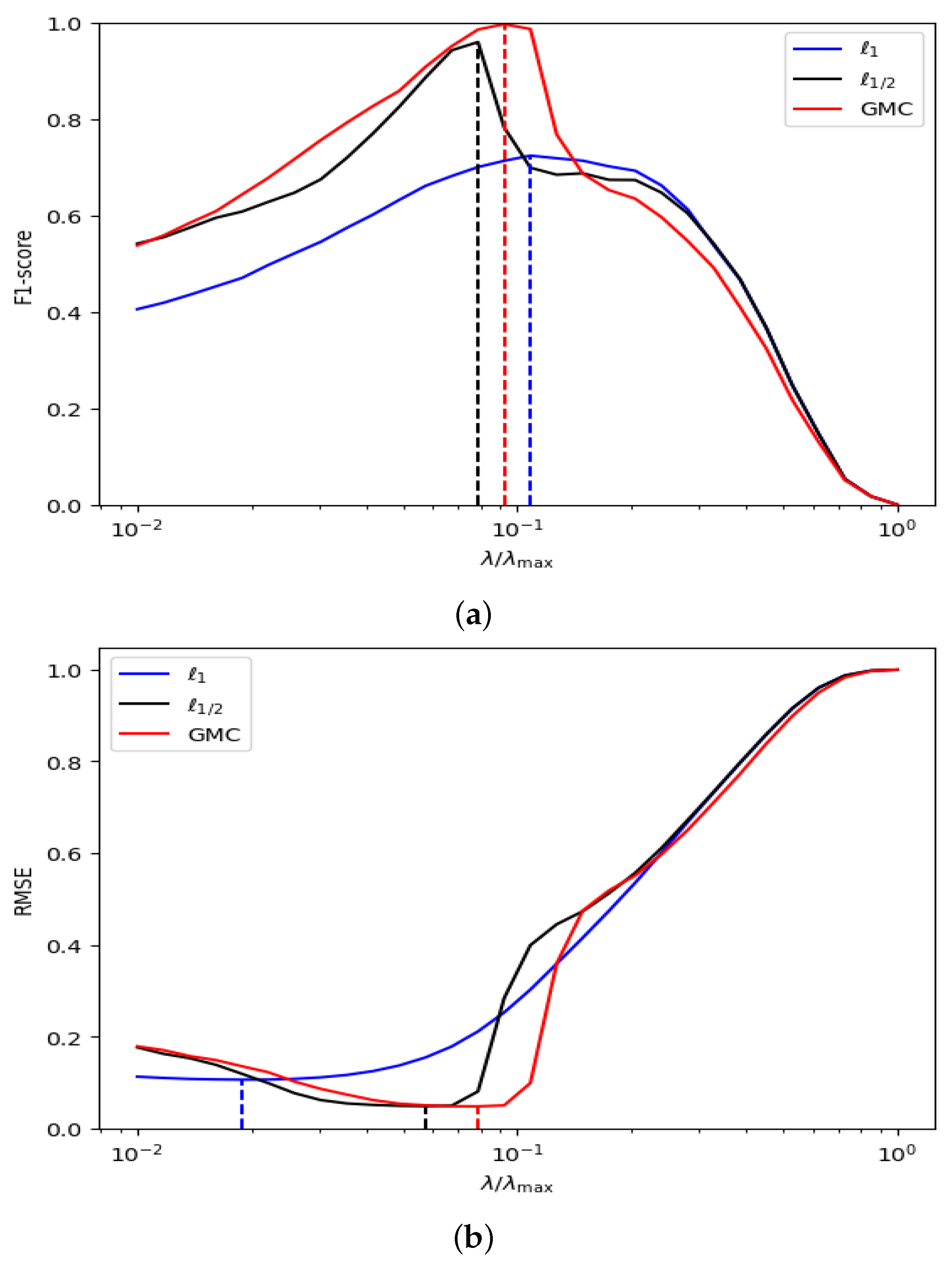
and calculated the average F1 and RMSE values. As shown in Figure 1a, when an appropriate λ value is selected, the F1 score of the GMC sparse regularization reaches the maximum value of 1. In contrast, the F1 scores of the 1 and 1 / 2 regularizations are approximately 0.7 and 0.95, respectively, both lower than the performance of the GMC regularization. Additionally, it can be clearly observed from Figure 1b that in the sparse vector prediction task, the minimum RMSE of the GMC sparse regularization is significantly lower than that of the 1 and 1 / 2 regularizations. This result further validates the superior accuracy of the GMC sparse regularization in sparse vector prediction. On the other hand, Figure 1 shows that when estimating sparse vectors, the difference between the λ values corresponding to the maximum F1 score and the minimum RMSE in the Lasso model based on GMC sparse regularization is relatively small. In contrast, this difference is larger in the 1 regularization, indicating that GMC sparse regularization (14) outperforms the 1 and 1 / 2 regularizations in terms of prediction performance when choosing an appropriate λ value.
The conclusion of our study highlights the exceptional predictive performance of our model (2) in estimating sparse vectors, surpassing the 1 regularization approach employed by the Lasso model. Additionally, although the Lasso model with 1 / 2 regularization also performs well in prediction tasks, its non-convexity poses challenges for the algorithms solving the objective function. In contrast, our model not only has excellent predictive ability but also ensures the overall convexity of the objective function, thereby providing convenient conditions for the design and implementation of optimization algorithms. In summary, the model proposed in this study has significant advantages in both predictive performance and optimization characteristics, effectively avoiding the computational difficulties brought by non-convex regularization methods.

4.2. MRI Reconstruction

The utilization of high-dimensional sparse linear regression serves as the foundation for numerous signal and image processing techniques, including MRI reconstruction [43,44,45]. The MRI is a powerful medical imaging technique, featuring high soft tissue contrast and the advantage of being radiation-free. It is widely used in clinical diagnosis and scientific research fields. In this experimental, we employ GMC sparse regularization (15) for MRI reconstruction and compare its performance against 1 and 1 / 2 regularization.
To make the statement clear, we define the design matrix X = R × F , where R R n × p is the sampling template, and F R p × p is the sparse Fourier operator. We tested different reconstruction models on three MRI images with variable density sampling and Cartesian sampling templates, respectively. For comparison, all images are set to 256 × 256 pixels, with grayscale values ranging from 0 to 255. The parameters were λ = 0.001 , ρ = 150 , the iteration step size α was chosen α = 1 . For the GMC regularization, it is necessary to explicitly specify matrix B and set it using (16) with ω = 0.9 .
In this experiment, we selected relative error (RE) and peak signal-to-noise ratio (PSNR) as evaluation metrics to quantitatively assess the quality and accuracy of reconstructed images.
The RE is defined as
RE = β ^ β * 2 β * 2 ,
where β * and β ^ are the original and reconstructed images, respectively.
The PSNR is defined as
PSNR = 10 · lg MAX 2 1 N β ^ β * 2 2 ,
where N = 256 × 256 , MAX = 255 , and β ^ , β * are the reconstructed, and the original image, respectively.
For these two types of quantitative evaluation criteria, the lower the RE value, the more superior the reconstruction effect, while for PSNR, an increase in numerical value indicates a more outstanding reconstruction ability.
To further enhance the visual contrast effect, we calculated the difference between the reconstructed image and the original image. Furthermore, we magnified a small portion of the local image to show more details. The reconstruction results of three regularizations are shown in Figure 2, Figure 3 and Figure 4. It can be found that the reconstructed images based on 1 regularization have problems such as blurred edges and residual shadows, and the 1 / 2 regularization reconstruction model also shows similar phenomena. In contrast, the reconstructed images based on GMC sparse regularization are closer to the original images and exhibit higher reconstruction quality.
Additionally, we conducted a quantitative evaluation of the reconstruction results in Table 1. It is obvious that compared with 1 and 1 / 2 regularization, GMC sparse regularization has the best performance in MRI reconstruction and can obtain the lowest RE and highest PSNR.

5. Conclusions

In this paper, we propose CNC sparse regularization as a valuable alternative to the 1 regularization used in Lasso regression. This approach effectively addresses the issue of underestimation for high-amplitude components while ensuring the global convexity of the objective function. Our theoretical analysis demonstrates that the prediction error bound associated with CNC sparse regularization is smaller than that of 1 regularization, which provides theoretical support for the practical application of the CNC regularization. Additionally, we demonstrate that the Lasso model with CNC regularization exhibits superior performance on both synthetic and real-world datasets. These findings suggest its potential significance in future applications such as image denoising, image reconstruction, seismic reflection analysis, etc.
Additionally, given that the oracle inequality of the Lasso model relies on the restricted eigenvalue condition, future research directions may include exploring theoretical guarantees under more relaxed assumptions, such as the oracle inequality based on weak correlation or unconstrained design matrices, and experimentally verifying the practical effectiveness of the restricted eigenvalue condition (such as calculating the specific value of κ T ), and further analyzing its impact on model performance.

Author Contributions

Conceptualization, W.C. and J.Z.; methodology, W.C.; software, W.C.; validation, Q.L. and H.L.; formal analysis, Q.L.; data curation, H.L.; writing—original draft preparation, W.C.; writing—review and editing, J.Z.; visualization, W.C.; supervision, J.Z.; project administration, J.Z.; funding acquisition, J.Z.. All authors have read and agreed to the published version of the manuscript.

Funding

This research was funded by the Undergraduate Training Program of Yangtze University for Innovation and Entrepreneurship (Yz2023302).

Data Availability Statement

The code for the proposed method in this paper are available upon request from the corresponding author.

Conflicts of Interest

The authors declare no conflict of interest. The funders had no role in the design of the study; in the collection, analyses, or interpretation of data; in the writing of the manuscript; or in the decision to publish the results.

Appendix A

Appendix A.1. Proof of Theorem 1

The proof of Theorem 1 follows the approach outlined in Theorem 2 from [12].
Proof. 
Firstly, we consider the first order optimality conditions of the convex problems (2). According to the chain rule of subdifferential, we can derive the subdifferential the 1 term is
β 1 = sgn ( β ) ,
where
sgn ( β ) = { 1 } , β > 0 , [ 1 , 1 ] , β = 0 , { 1 } , β < 0 .
Using the Karush–Kuhn–Tucker conditions, we have
1 n β X ( y X β ^ ) λ sgn ( β ) .
This implies that for any β ¯ R p , we obtain
1 n β ^ X ( y X β ^ ) = λ β ^ 1 ,
and
1 n β ¯ X ( y X β ^ ) = λ β ¯ 1 .
Subtracting (A1) from (A2), we obtain
1 n ( β ¯ β ^ ) X ( y X β ^ ) λ ( β ¯ 1 β ^ 1 ) .
By utilizing the observation model y = X β * + ϵ and considering polarization equality, i.e., 2 u v = u 2 2 + v 2 2 u v 2 2 , the above Equation (A3) can be rewritten as
1 n X ( β ¯ β ^ ) 2 2 + 1 n X ( β * β ^ ) 2 2 1 2 n X ( β ¯ β ^ ) X ( β * β ^ ) 2 2 + 1 n ϵ X ( β ^ β ¯ ) + 2 λ β ¯ 1 2 λ β ^ 1 .
Let us first consider ϵ X ( β ^ β ¯ ) and apply Holder’s inequality, we have
ϵ X ( β ^ β ¯ ) = ( X β ^ X β ¯ ) ( I Π T ) ϵ + ( X β ^ X β ¯ ) Π T ϵ   X ( I Π T ) ϵ ·   β ^ β ¯ 1 +   Π T ϵ 2 · X ( β ^ β ¯ ) 2 .
The classical results for the standard Gaussian tail distribution and the χ 2 distribution demonstrate that, given any T, there exists a probability of at least 1 2 δ satisfying the following two inequalities [46]
X ( I Π T ) ϵ γ σ 2 log ( p δ ) = λ n ,
Π T ϵ 2 σ * | T | + 2 log ( 1 δ ) .
Next, note that for any set T, β 1 = β T 1 + β T c 1 . Then, using the triangle inequality and subadditivity of β 1 , we have
β ^ β ¯ 1 + β ¯ 1 β ^ 1 2 ( β ^ β ¯ ) T 1 + 2 β ¯ T c 1 .
Furthermore, by employing the definition of compatibility, we can deduce the following fact:
β ^ β ¯ 1 κ T 1 | T | / n X ( β ^ β ¯ ) 2 .
Combining (A4)–(A9) leads to the following inequality
1 n X ( β ¯ β ^ ) 2 2 + 1 n X ( β * β ^ ) 2 2 1 2 n X ( β ¯ β ^ ) X ( β * β ^ ) 2 2 + 2 1 n Π T ϵ 2 · X ( β ^ β ¯ ) 2 + 4 λ κ T 1 | T | / n · X ( β ^ β ¯ ) 2 + 4 λ β T c 1 .
By employing Young’s inequality, which is 2 u v u 2 / e + e v 2 for e > 0 , with u = Π ϵ 2 + 2 λ κ T 1 | T | / n , v =   X ( β ^ β ¯ ) 2 , and e = 1 n , we have
2 1 n Π T ϵ 2 + 2 λ κ T 1 | T | / n X ( β ^ β ¯ ) 2 n 1 n Π T ϵ 2 + 2 λ κ T 1 | T | / n 2 + 1 n X ( β ^ β ¯ ) 2 2 .
Therefore, the (A10) can be rewritten as
1 n X ( β * β ^ ) 2 2 1 2 n X ( β ¯ β ^ ) X ( β * β ^ ) 2 2 + 4 λ β T c 1 + n 1 n Π T ϵ 2 + 2 λ κ T 1 | T | / n 2 .
The substitution of (A7) into (A12) results in
1 n X ( β * β ^ ) 2 2 1 2 n X ( β ¯ β ^ ) X ( β * β ^ ) 2 2 + 4 λ β T c 1 + σ * 2 n | T | + 2 log ( 1 δ ) + 8 γ 2 log ( p / δ ) κ T 2 .

Appendix A.2. Proof of Theorem 2

Proof. 
By plugging the GMC regularization (7) into F B G M C ( β ) , we can rewrite F B G M C ( β ) as
F B G M C ( β ) = 1 2 n y X β 2 2 + λ β 1 λ min v v 1 + 1 2 B ( β v ) 2 2 = max v 1 2 n y X β 2 2 + λ β 1 λ v 1 λ 2 B ( β v ) 2 2 = max v { 1 2 β ( 1 n X X λ B B ) β + λ β 1 + 1 2 n y 2 2 1 n y X β v 1 λ 2 B v 2 2 + λ v B B β } = 1 2 β ( 1 n X X λ B B ) β + λ β 1 + 1 2 n y 2 2 1 n y X β + λ max v v 1 λ 2 B v 2 2 + λ v B B β .
The expression enclosed in the curly braces in (A14) is affine with respect to β (hence convex). Consequently, the final term in the equation is also convex, as it represents the pointwise maximum of a collection of convex functions. Therefore, F ( β ) is convex if 1 n X X λ B B 0 , and if 1 n X X λ B B 0 , then F B G M C ( β ) demonstrates strict convexity. ☐

Appendix A.3. Proof of Theorem 3

Proof. 
We first use the Karush–Kuhn–Tucker conditions to infer that
0 β f ( β ) | β = β ^ = 1 n ( X T y X X β ^ ) + β Ψ B G M C ( β ) | β = β ^ .
Using the chain rule, β Ψ B G M C ( β ) | β = β ^ = sgn ( β ) + B B β arg min v v 1 + 1 2 ( β v ) 2 2 . Then, using (A15), we also can see that there exists z = sgn ( β ) + B B β arg min v v 1 + 1 2 ( β v ) 2 2 , such that
1 n X ( y X β ^ ) = λ z .
Specifically, β ¯ R p , we have
1 n β ¯ X ( y X β ^ ) = λ β ¯ z ,
and
1 n β ^ X ( y X β ^ ) = λ β ^ z .
Subtracting (A17) from (A16), and then using the subgradient definition, we can get
1 n ( β ¯ β ^ ) X ( y X β ^ ) = λ ( β ¯ β ^ ) z λ Ψ B G M C ( β ¯ ) Ψ B G M C ( β ^ ) .
By utilizing the observation model y = X β * + ϵ and considering polarization equality, i.e., 2 u v = u 2 2 + v 2 2 u v 2 2 , the left side of Equation (A18) can be represented as
1 n ( β ¯ β ^ ) X ( X β * + ϵ X β ^ )
= 1 n ( β ¯ β ^ ) X X ( β * β ^ ) + 1 n ϵ X ( β ¯ β ^ ) = 1 2 n X ( β ¯ β ^ ) 2 2 + 1 2 n X ( β * β ^ ) 2 2 1 2 n X ( β ¯ β ^ ) X ( β * β ^ ) 2 2 + 1 n ϵ X ( β ¯ β ^ ) .
Let us introduce the two difference vectors δ = β ^ β * and δ ¯ = β ^ β ¯ . Thus, for every T [ P ] , combining (A19), (A18) with the decomposition ϵ = Π T ϵ + ( I n Π T ) ϵ yields
1 n X δ ¯ 2 2 + 1 n X δ 2 2 1 n X δ ¯ X δ 2 2 + 2 n ϵ X δ ¯ + 2 λ Ψ B G M C ( β ¯ ) 2 λ Ψ B G M C ( β ^ ) .
Applying Holder’s inequality to ϵ X δ ¯ in (A20), we can obtain
( X δ ¯ ) ϵ = ( X δ ¯ ) ( I Π T ) ϵ + ( X δ ¯ ) Π T ϵ
  X ( I Π T ) ϵ   · δ ¯ 1   + Π T ϵ 2 · X δ ¯ 2 .
The classical results for the standard Gaussian tail distribution and the χ 2 distribution demonstrate that, given any T, there exists a probability of at least 1 2 δ satisfying the following two inequalities [46]
X ( I Π ) ϵ γ σ 2 log ( p δ ) = λ n ,
Π T ϵ 2 σ * | T | + 2 log ( 1 δ ) .
Then, using λ β 1 λ Ψ σ m a x I G M C ( β ) + μ 2 β 2 2 and (A22), we can further bound (A21) as follows
2 n ( X δ ¯ ) ϵ 2 n X ( I Π T ) ϵ · δ ¯ 1 + 2 n Π T ϵ 2 · X δ ¯ 2 2 n Π T ϵ 2 · X δ ¯ 2 + 2 λ Ψ σ m a x I G M C ( β ^ β ¯ ) + μ β ^ β ¯ 2 2 .
For non-separable regularizers, we can easily obtain
Ψ B G M C ( β ¯ ) = β ¯ 1 min v v 1 + 1 2 B ( β ¯ v ) 2 2 Ψ σ m i n I G M C ( β ¯ ) ,
and
Ψ B G M C ( β ^ ) = β ^ 1 min v v 1 + 1 2 B ( β ^ v ) 2 2 Ψ σ m a x I G M C ( β ^ ) .
Together with X X = I , and X X δ ¯ 2 2   X 2 2 X δ ¯ 2 2 , the bound (A20) can be rewritten as
1 n X δ ¯ 2 2 + 1 n X δ 2 2 1 n X δ ¯ X δ 2 2 + 2 n Π T ϵ 2 · X δ ¯ 2
+ 2 λ Ψ σ m a x I G M C ( β ^ β ¯ ) + 2 λ Ψ σ m i n I G M C ( β ¯ ) 2 λ Ψ σ m a x I G M C ( β ^ ) + μ X 2 2 X δ ¯ 2 2 .
Note that for any set T, Ψ b I G M C ( β ) = Ψ b I G M C ( ( β ) T ) + Ψ b I G M C ( ( β ) T c ) . Subsequently, according to the triangle inequality, as well as the subadditivity and symmetry of Ψ b G M C , we derive
Ψ σ m a x I G M C ( β ^ β ¯ ) + Ψ σ m i n I G M C ( β ¯ ) Ψ σ m a x I G M C ( β ^ ) Ψ σ m a x I G M C ( ( β ^ β ¯ ) T ) + Ψ σ m a x I G M C ( β ^ T c ) + Ψ σ m a x I G M C ( β ¯ T c ) + Ψ σ m i n I G M C ( β ¯ ) Ψ σ m a x I G M C ( β ^ T ) Ψ σ m a x I G M C ( β ^ T c )
Ψ σ m i n I G M C ( ( β ^ β ¯ ) T ) + 2 Ψ σ m i n I G M C ( ( β ¯ ) T c ) + Ψ σ m i n I G M C ( ( β ¯ ) T ) Ψ σ m a x I G M C ( β ^ T ) 2 Ψ σ m i n I G M C ( ( β ^ β ¯ ) T ) + 2 Ψ σ m i n I G M C ( ( β ¯ ) T c ) .
The constraint (A26) is further refined by the compatibility factor,
Ψ σ m i n I G M C ( ( β ^ β ¯ ) T )   ( β ^ β ¯ ) T 1 κ T 1 | T | / n X ( β ^ β ¯ ) 2 .
Next, by combining Equations (A25)–(A27), we can obtain
1 n X δ ¯ 2 2 + 1 n X δ 2 2 1 n X δ ¯ X δ 2 2 + 2 1 n Π T ϵ 2 + 2 λ κ T 1 | T | / n X δ ¯ 2 + 4 λ Ψ σ m i n I G M C ( ( β ¯ ) T c ) + μ X 2 2 X δ ¯ 2 2 .
By employing Young’s inequality, for any positive value of e > 0 , the inequality 2 a b a 2 e + e b 2 holds true, with a = 1 n Π T ϵ 2 + 2 λ κ T 1 | T | / n , b = X δ ¯ 2 , and e = 1 n μ X 2 2 we have
2 1 n Π T ϵ 2 + 2 λ κ T 1 | T | / n X δ ¯ 2 1 e 1 n Π T ϵ 2 + 2 λ κ T 1 | T | / n 2 + e X δ ¯ 2 2 2 1 n μ X 2 2 1 n 2 Π T ϵ 2 2 + 1 n 4 λ 2 κ T 2 | T | + ( 1 n μ X 2 2 ) X δ ¯ 2 2 .
Therefore,
1 n X δ 2 2 1 n X δ ¯ X δ 2 2 + 4 λ Ψ σ m i n I G M C ( ( β ¯ ) T c ) + 2 1 n μ X 2 2 1 n 2 Π T ϵ 2 2 + 1 n 4 λ 2 κ T 2 | T | .
The substitution of Equation (A23) into Equation (A29) yields
1 n X δ 2 2 1 n X δ ¯ X δ 2 2
+ 4 λ Ψ σ m i n I G M C ( ( β ¯ ) T c ) + 2 σ * 2 n ( 1 n μ X 2 2 ) | T | + 2 log ( 1 / δ ) + 8 γ 2 log ( p / δ ) | T | κ T 2 .
Therefore, Theorem 3 is proven.

Appendix A.4. Proof of Theorem 4

The proof of Theorem 4 is drawing inspiration from Proposition 1 in [47].
Proof. 
According to Corollary 1, it can be easily observed that there exists μ 0 such that inequality λ Ψ B G M C + μ 2 β 2 2 0 is convex.
Now consider the augmented Lagrangian L ( β , z , u ) with regard to z as follows
L ( β , z , u ) = 1 2 n y X β 2 2 + λ Ψ B G M C ( z ) + u ( z β ) + ρ 2 z β 2 2 = λ Ψ B G M C ( z ) + ρ 2 z 2 2 u z + 1 2 n y X β 2 2 ρ u β + ρ 2 β 2 2 .
Note that 1 2 n y X β 2 2 ρ u β + ρ 2 β 2 2 is independent of z. Given the choice of ρ μ , L ( β , z , u ) is convex with respect to each of β , z and u. Therefore, Algorithm 1 can converge to limit points β * , z * , and u * .
The implication is that the dual residual lim k s ( k + 1 ) = ρ ( z * z * ) 2 = 0 . Regarding the primal residual, it can be observed from the u update step in line 6 of Algorithm 1 that for all k , t 0 ,
u ( k + t ) = u ( k ) + i = 1 t ( β ( k + i ) z ( k + i ) ) .
For fixed t and as k , we have
u * = u * + t ( β * z * ) ,
holds t 0 . Thus, β * z * = 0 , and therefore lim k r ( k ) = β * z * 2 = 0 . ☐

References

  1. Tibshirani, R. Regression shrinkage and selection via the lasso. J. R. Stat. Soc. Ser. B Stat. Methodol. 1996, 58, 267–288. [Google Scholar] [CrossRef]
  2. Zhao, P.; Yu, B. On Model Selection Consistency of Lasso. J. Mach. Learn. Res. 2006, 7, 2541–2563. [Google Scholar]
  3. Hastie, T.; Tibshirani, R.; Wainwright, M. Statistical Learning with Sparsity: The Lasso and Generalizations; CRC Press: Boca Raton, FL, USA, 2015. [Google Scholar]
  4. Chen, S.S.; Donoho, D.L.; Saunders, M.A. Atomic decomposition by basis pursuit. SIAM Rev. 2001, 43, 129–159. [Google Scholar] [CrossRef]
  5. Adamek, R.; Smeekes, S.; Wilms, I. Lasso Inference for High-Dimensional Time Series. J. Econom. 2023, 235, 1114–1143. [Google Scholar] [CrossRef]
  6. Lee, H.; Hwang, T.; Oh, M.-h. Lasso Bandit with Compatibility Condition on Optimal Arm. In Proceedings of the Thirteenth International Conference on Learning Representations, Singapore, 24–28 April 2025. [Google Scholar]
  7. Ogundimu, E.O. On Lasso and adaptive Lasso for non-random sample in credit scoring. Stat. Model. 2024, 24, 115–138. [Google Scholar]
  8. Bruckstein, A.M.; Donoho, D.L.; Elad, M. From sparse solutions of systems of equations to sparse modeling of signals and images. SIAM Rev. 2009, 51, 34–81. [Google Scholar]
  9. Zanon, M.; Zambonin, G.; Susto, G.A.; McLoone, S. Sparse Logistic Regression: Comparison of Regularization and Bayesian Implementations. Algorithms 2020, 13, 137. [Google Scholar] [CrossRef]
  10. Kayanan, M.; Wijekoon, P. Improved LARS algorithm for adaptive LASSO in the linear regression model. Asian J. Probab. Stat. 2024, 26, 86–95. [Google Scholar] [CrossRef]
  11. Iloska, M.; Djurić, P.M.; Bugallo, M.F. Fast Sparse Learning from Streaming Data with LASSO. In Proceedings of the 2025 IEEE International Conference on Acoustics, Speech and Signal Processing (ICASSP), Hyderabad, India, 6–11 April 2025. [Google Scholar]
  12. Dalalyan, A.S.; Hebiri, M.; Lederer, J. On the Prediction Performance of the Lasso. Bernoulli 2017, 23, 552–581. [Google Scholar] [CrossRef]
  13. Donoho, D.L.; Elad, M.; Temlyakov, V.N. Stable recovery of sparse overcomplete representations in the presence of noise. IEEE Trans. Inf. Theory 2005, 52, 6–18. [Google Scholar]
  14. Candès, E.J.; Romberg, J.K.; Tao, T. Stable signal recovery from incomplete and inaccurate measurements. Commun. Pure Appl. Math. 2010, 59, 1207–1223. [Google Scholar]
  15. Zhang, C.H. Nearly unbiased variable selection under minimax concave penalty. Ann. Stat. 2010, 38, 894–942. [Google Scholar] [CrossRef] [PubMed]
  16. Zou, H. The adaptive lasso and its oracle properties. J. Am. Stat. Assoc. 2006, 101, 1418–1429. [Google Scholar] [CrossRef]
  17. Basu, A.; Ghosh, A.; Jaenada, M.; Pardo, L.; Proietti, T. Robust adaptive LASSO in high-dimensional logistic regression. Stat. Methods Appl. 2024, 33, 1217–1249. [Google Scholar] [CrossRef]
  18. Fan, J.; Li, R. Variable selection via nonconcave penalized likelihood and its oracle properties. J. Am. Stat. Assoc. 2001, 96, 1348–1360. [Google Scholar] [CrossRef]
  19. Lanza, A.; Morigi, S.; Selesnick, I.W.; Sgallari, F. Convex non-convex variational models. In Handbook of Mathematical Models and Algorithms in Computer Vision and Imaging: Mathematical Imaging and Vision; Springer: Cham, Switzerland, 2022; pp. 1–57. [Google Scholar]
  20. Selesnick, I. Sparse regularization via convex analysis. IEEE Trans. Signal Process. 2017, 65, 4481–4494. [Google Scholar] [CrossRef]
  21. Selesnick, I.; Lanza, A.; Morigi, S.; Sgallari, F. Non-convex total variation regularization for convex denoising of signals. J. Math. Imaging Vis. 2020, 62, 825–841. [Google Scholar] [CrossRef]
  22. Zou, J.; Shen, M.; Zhang, Y.; Li, H.; Liu, G.; Ding, S. Total variation denoising with non-convex regularizers. IEEE Access 2018, 7, 4422–4431. [Google Scholar] [CrossRef]
  23. Selesnick, I. Total variation denoising via the Moreau envelope. IEEE Signal Process. Lett. 2017, 24, 216–220. [Google Scholar] [CrossRef]
  24. Lanza, A.; Morigi, S.; Selesnick, I.; Sgallari, F. Sparsity-inducing nonconvex nonseparable regularization for convex image processing. SIAM J. Imaging Sci. 2019, 12, 1099–1134. [Google Scholar] [CrossRef]
  25. Shen, M.; Li, J.; Zhang, T.; Zou, J. Magnetic resonance imaging reconstruction via non-convex total variation regularization. Int. J. Imaging Syst. Technol. 2021, 31, 412–424. [Google Scholar] [CrossRef]
  26. Li, J.; Li, J.; Xie, Z.; Zou, J. Plug-and-play ADMM for MRI reconstruction with convex nonconvex sparse regularization. IEEE Access 2021, 9, 148315–148324. [Google Scholar] [CrossRef]
  27. Li, J.; Xie, Z.; Liu, G.; Yang, L.; Zou, J. Diffusion optical tomography reconstruction based on convex–nonconvex graph total variation regularization. Math. Methods Appl. Sci. 2023, 46, 4534–4545. [Google Scholar] [CrossRef]
  28. Xu, Y.; Qu, M.; Liu, L.; Liu, G.; Zou, J. Plug-and-play algorithms for convex non-convex regularization: Convergence analysis and applications. Math. Methods Appl. Sci. 2024, 47, 1577–1598. [Google Scholar] [CrossRef]
  29. Xu, Z.; Chang, X.; Xu, F.; Zhang, H. L_{1/2} regularization: A thresholding representation theory and a fast solver. IEEE Trans. Neural Netw. Learn. Syst. 2012, 23, 1013–1027. [Google Scholar]
  30. Wen, F.; Chu, L.; Liu, P.; Qiu, R.C. A survey on nonconvex regularization-based sparse and low-rank recovery in signal processing, statistics, and machine learning. IEEE Access 2018, 6, 69883–69906. [Google Scholar] [CrossRef]
  31. Woodworth, J.; Chartrand, R. Compressed sensing recovery via nonconvex shrinkage penalties. Inverse Probl. 2016, 32, 075004. [Google Scholar] [CrossRef]
  32. Selesnick, I.W.; Bayram, I. Sparse Signal Estimation by Maximally Sparse Convex Optimization. IEEE Trans. Signal Process. 2014, 62, 1078–1092. [Google Scholar] [CrossRef]
  33. Al-Shabili, A.H.; Feng, Y.; Selesnick, I. Sharpening sparse regularizers via smoothing. IEEE Open J. Signal Process. 2021, 2, 396–409. [Google Scholar] [CrossRef]
  34. Lanza, A.; Morigi, S.; Selesnick, I.; Sgallari, F. Nonconvex nonsmooth optimization via convex–nonconvex majorization–minimization. Numer. Math. 2017, 136, 343–381. [Google Scholar] [CrossRef]
  35. Bunea, F.; Tsybakov, A.B.; Wegkamp, M.H. Aggregation and sparsity via 1 penalized least squares. In Proceedings of the 19th Annual Conference on Learning Theory, Pittsburgh, PA, USA, 22–25 June 2006; COLT’06. pp. 379–391. [Google Scholar] [CrossRef]
  36. Bunea, F.; Tsybakov, A.B.; Wegkamp, M.H. Aggregation for Gaussian regression. Ann. Stat. 2007, 35, 1674–1697. [Google Scholar]
  37. Bunea, F.; Tsybakov, A.; Wegkamp, M. Sparsity oracle inequalities for the Lasso. Electron. J. Stat. 2007, 1, 169–194. [Google Scholar] [CrossRef]
  38. Bickel, P.J.; Ritov, Y.; Tsybakov, A. Simultaneous Analysis of Lasso and Dantzig Selector. Ann. Stat. 2009, 37, 1705–1732. [Google Scholar]
  39. Koltchinskii, V.; Lounici, K.; Tsybakov, A.B. Nuclear-norm penalization and optimal rates for noisy low-rank matrix completion. Ann. Stat. 2011, 39, 2302–2329. [Google Scholar]
  40. Sun, T.; Zhang, C.H. Scaled sparse linear regression. Biometrika 2012, 99, 879–898. [Google Scholar]
  41. Parikh, N.; Boyd, S. Proximal algorithms. Found. Trends® Optim. 2014, 1, 127–239. [Google Scholar]
  42. Boyd, S.; Parikh, N.; Chu, E.; Peleato, B.; Eckstein, J. Distributed optimization and statistical learning via the alternating direction method of multipliers. Found. Trends® Mach. Learn. 2010, 3, 1–122. [Google Scholar]
  43. Lustig, M.; Donoho, D.; Pauly, J.M. Sparse MRI: The application of compressed sensing for rapid MR imaging. Magn. Reson. Med. 2007, 58, 1182–1195. [Google Scholar] [CrossRef]
  44. Lustig, M.; Donoho, D.L.; Santos, J.M.; Pauly, J.M. Compressed sensing MRI. IEEE Signal Process. Mag. 2008, 25, 72–82. [Google Scholar]
  45. Fessler, J.A. Optimization Methods for Magnetic Resonance Image Reconstruction: Key Models and Optimization Algorithms. IEEE Signal Process. Mag. 2020, 37, 33–40. [Google Scholar]
  46. Wainwright, M.J. High-Dimensional Statistics: A Non-Asymptotic Viewpoint; Cambridge University Press: Cambridge, UK, 2019. [Google Scholar]
  47. Ma, S.; Huang, J. A concave pairwise fusion approach to subgroup analysis. J. Am. Stat. Assoc. 2017, 112, 410–423. [Google Scholar]
Figure 1. Regularization paths. (a) F1 score, (b) RMSE. The red solid line, black solid line, and blue solid line represent the Lasso model (14) with GMC, 1 / 2 , and 1 regularization, respectively. The red dotted line, black dotted line, and blue dotted line correspond to the values of λ / λ m a x when the maximum F1 score and the minimum RMSE are achieved in the support recovery process for the Lasso model with GMC, 1 / 2 , and 1 regularization, respectively.
Algorithms 18 00195 g001
Figure 2. (a), Original image; (b), undersampling template with 30 % sampling rate; (ce), reconstructed images using 1 regularization, 1 / 2 regularization and GMC regularization, respectively; (f), difference between (a) and (c); (g), difference between (a) and (d); (h), difference between (a) and (e).
Algorithms 18 00195 g002
Figure 3. (a), Original image; (b), undersampling template with 30 % sampling rate; (ce), reconstructed images using 1 regularization, 1 / 2 regularization and GMC regularization, respectively; (f), difference between (a) and (c); (g), difference between (a) and (d); (h), difference between (a) and (e).
Algorithms 18 00195 g003
Figure 4. (a), Original image; (b), undersampling template with 30 % sampling rate; (ce), reconstructed images using 1 regularization, 1 / 2 and GMC regularization, respectively; (f), difference between (a) and (c); (g), difference between (a) and (d); (h), difference between (a) and (e).
Algorithms 18 00195 g004
Table 1. Quantitative results of different regularizations. The best results are highlighted in bold.
TemplateImageModelREPSNR (dB)
Variable Density
Sampling
Image1 1 0.045835.6637
1 / 2 0.035637.8626
GMC0.027740.0481
Variable Density
Sampling
Image2 1 0.091231.3563
1 / 2 0.079732.5274
GMC0.064834.3238
Cartesian
Sampling
Image3 1 0.107629.8075
1 / 2 0.095230.8666
GMC0.086631.6867
Disclaimer/Publisher’s Note: The statements, opinions and data contained in all publications are solely those of the individual author(s) and contributor(s) and not of MDPI and/or the editor(s). MDPI and/or the editor(s) disclaim responsibility for any injury to people or property resulting from any ideas, methods, instructions or products referred to in the content.

