An Optimal Scheduling Model for Connected Automated Vehicles at an Unsignalized Intersection

Abstract

The application of connected automated vehicles (CAVs) provides new opportunities and challenges for optimizing and controlling urban intersections. To avoid collisions of vehicles in conflicting directions at intersections and improve the efficiency of intersections, an optimal scheduling model for CAVs at an unsignalized intersection is proposed. The model develops a linear programming model of intersection vehicle timing with the minimum average vehicle delay within the optimization time window as the optimization objective and the minimum safe time interval for vehicles to pass through the intersection as the constraint. A rolling optimization algorithm is designed to improve the efficiency of the algorithm solution. Finally, the effects of different traffic demand conditions on the results are investigated based on numerical simulation experiments. The results show that both the proposed algorithm and the Gurobi solver can significantly reduce the average vehicle delay compared with the first-come-first-served (FCFS) control method, and the proposed model and algorithm can reduce the average vehicle delay by 76.22% at most. Compared with the Gurobi solver, the proposed model and algorithm can reduce the solution time and ensure the optimization effect to the greatest extent. Therefore, the proposed model and algorithm provide theoretical support for managing CAVs at unsignalized intersections.

1. Introduction

1.1. Research Background

As major bottlenecks in cities, intersections are often prone to traffic congestion and accidents [1,2,3]. Traffic signal control is commonly employed at intersections to spatially and temporally separate vehicles, thereby preventing vehicle conflicts. In recent years, the development of vehicle–infrastructure cooperated autonomous driving has facilitated the implementation of connected automated vehicles (CAVs) [4,5,6,7]. Existing research [8,9,10,11] indicates that the application of CAVs can enhance traffic efficiency and significantly improve traffic safety. Therefore, studying intersection control in the connected automated environment is beneficial for improving the traffic flow efficiency at intersections [12,13,14,15].

1.2. Literature Review

Traditional methods to avoid vehicle conflicts at intersections generally include two approaches. The first involves setting up traffic signals, which use signal control to separate vehicles in both time and space, thereby preventing conflicts [16,17,18,19,20]. Huang et al. [16] proposed a reservation-based traffic signal control method for mixed traffic flow at intersections. The simulation results showed that the proposed method is superior to the actuated traffic signal control. Yao et al. [17] developed a dynamic predictive traffic signal control framework in a cross-sectional vehicle infrastructure integration environment. The results showed that, compared with the traditional full-actuated control, the proposed method can reduce the average delay and queue length by up to 33% and 35%, respectively. Yao et al. [18] proposed a cell transmission model (CTM)-based traffic signal timing of mixed traffic flow with connected automated vehicles. The results show that the proposed model can effectively reduce the range and dissipation time of traffic congestion. Mirchandani et al. [19] developed a real-time traffic signal control system. Moreover, Feng et al. [20] proposed a real-time adaptive traffic signal control in a connected vehicle environment. The simulation results showed that the proposed algorithm outperforms actuated control by reducing the total delay by as much as 16.33% in a high-penetration rate case and by a similar amount in a low-penetration rate case.

The second approach involves placing stop signs at the entrance to intersections and requiring vehicles entering the intersection to stop and yield when their path conflicts with vehicles already within the intersection [21,22,23,24]. Brilon and Wu [21] developed a new simplified theoretical approach for the determination of capacities at unsignalized intersections. Heidemann and Wegmann [22] proposed a general queueing theory model for traffic flow at unsignalized intersections. The numerical results showed that the proposed model can capture the traffic flow at unsignalized intersections. Krbálek et al. [23] developed statistical aspects of gap acceptance theory for investigating unsignalized intersection capacity. Moreover, this paper estimated an implicit acceptance rule, with the help of a situation in which a minor street driver is deciding on the acceptance/rejection of an offered priority clearance. Li et al. [24] investigated the phase diagrams of traffic states induced by the bottleneck of an unsignalized intersection, which consists of two perpendicular one-lane roads. The results of the theoretical analysis are in good agreement with the computer simulation.

Consequently, the first method is suitable for any scenario, while the second only applies to situations with low intersection traffic flow. With the advancement of vehicle–infrastructure cooperated autonomous driving, some scholars have attempted to optimize the sequence of vehicles passing through intersections to avoid conflicts [25,26,27,28,29]. These methods can also be divided into two categories. The first is based on traffic signal optimization, emphasizing collaborative optimization between vehicles and traffic signals [30,31,32]. The second assumes all vehicles are CAVs, eliminating the need for traffic signals at intersections. Instead, it only requires assigning a reasonable sequence for vehicles to arrive at the intersection, thereby preventing conflicts between vehicles [33,34,35]. For the second control method, the main issues in existing research are as follows: (1) when the optimization time window is long, the algorithm takes a considerable amount of time to solve, resulting in low efficiency; (2) the connection between different optimization time windows is not considered, making the algorithm theoretical and difficult to apply in practice; and (3) the influence mechanism of the key model parameters on the results is not analyzed.

1.3. Main Contributions

To address this issue, this paper constructs a linear programming-based model for optimizing the sequence of vehicles passing through intersections. A rolling optimization algorithm is designed to solve the model and enhance its solving efficiency. Therefore, the main contributions of this paper are as follows:

(1) The traffic control of the unsignalized intersection is abstracted as a vehicle sequence optimization problem. On this basis, a linear programming model is developed.

(2) An efficient algorithm is designed to ensure the accuracy and speed of the solution based on moving horizon optimization.

(3) A numerical experiment is conducted to analyze the impact of critical parameters on the control effect.

1.4. The Structure of This Paper

The remainder of this paper is organized as follows. Section 2 describes and analyzes the problem to be solved. Section 3 develops an optimization model for this problem and designs a solving algorithm. Section 4 designs numerical analysis experiments to discuss the effectiveness of the proposed model and algorithm. Finally, Section 5 presents the conclusions of this paper.

2. Modeling Preparation

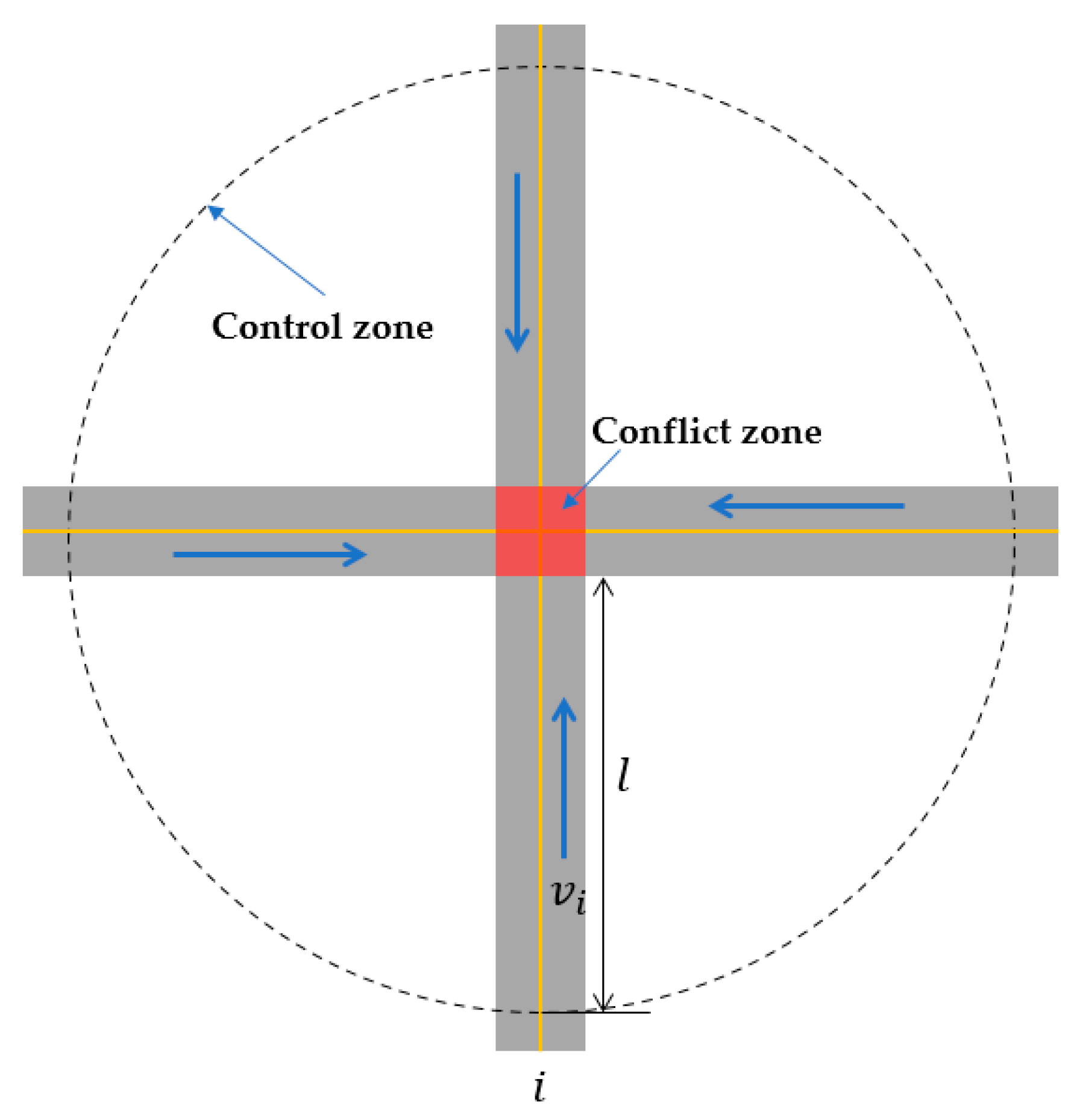
2.1. Problem Description

As shown in Figure 1, this is a typical unsignalized intersection. Lane changing is not considered in this paper, mainly because it is generally prohibited for vehicles to change lanes at the entrance of intersections [13,14]. In addition, readers can refer to the research on optimizing lane changing of CAVs [32]. Moreover, we only consider isolated intersections. Cooperative control can be implemented for intersections that are very close in distance [36]. Vehicle turns are not considered here to facilitate modeling. According to Figure 1, when vehicles pass through an unsignalized intersection, conflicts exist in different directions. Starting from the north direction, let $i\in \mathcal{I}=\left\{\mathrm{1,2},\mathrm{3,4}\right\}$ represent the four different directions. Then, the set of conflicting directions can be represented as $\mathcal{C}=\left\{\left(\mathrm{1,2}\right),\left(\mathrm{1,4}\right),\left(\mathrm{2,3}\right),\left(\mathrm{3,4}\right)\right\}$. To ensure the safe passage of vehicles through the intersection, we assume that vehicles from conflicting directions cannot simultaneously appear in the conflict zone at the same time. If the intersection adopts a Vehicle-to-Infrastructure (V2I) control mode, the length of the control zone is $l$, and the free-flow speed of each road segment at the intersection is $v_i,i\in \mathcal{I}$. For a given optimization time window $T$, let ${\mathcal{N}}_i$ represent the set of vehicles entering the control zone from the i-th direction within the optimization time window, where $j\in {\mathcal{N}}_i=\left\{\mathrm{1,2},\cdots ,\left|{\mathcal{N}}_i\right|\right\},i\in \mathcal{I}$. Suppose $t_{ij}^{-}$ and $t_{ij}^{+}$ represent the times when the j-th vehicle from the i-th direction enters the control zone and the conflict zone, respectively. The problem to be solved in this paper is to optimize the time $t_{ij}^{+}$ for vehicles entering the conflict zone of the intersection within the optimization time window, while ensuring vehicle safety, to reduce vehicle delays.

2.2. Problem Analysis

Assuming a four-way unsignalized intersection, within the optimization time window, there are only two vehicles in each direction, i.e.,$\left|{\mathcal{N}}_i\right|=2,i\in \mathcal{I}=\left\{\mathrm{1,2},\mathrm{3,4}\right\}$. According to permutation and combination theory, the total number of sequential combinations for these vehicles to pass through the intersection’s conflict zone is $A_8^8$. However, considering that vehicles from the same direction can only pass through the conflict zone in their order of arrival, the actual feasible passing sequences are $A_8^8/\left(A_2^2{A}_2^2{A}_2^2{A}_2^2\right)$. In summary, when the number of vehicles in each direction is $\left|{\mathcal{N}}_i\right|,i\in \mathcal{I}=\left\{\mathrm{1,2},\mathrm{3,4}\right\}$, the total number of feasible passing sequences is $A_{\sum _{i\in \mathcal{I}}\left|{\mathcal{N}}_i\right|}^{\sum _{i\in \mathcal{I}}\left|{\mathcal{N}}_i\right|}/\prod _{i\in \mathcal{I}}{A}_{\left|{\mathcal{N}}_i\right|}^{\left|{\mathcal{N}}_i\right|}$.

Theoretically, one could first enumerate all possible passing sequence combinations, then calculate the delay for each passing sequence, and select the passing sequence with the minimum delay as the optimal one. The number of passing sequence combinations increases exponentially with the number of vehicles. When there are two vehicles in each direction, the number of sequence combinations for vehicles passing through the intersection’s conflict zone already reaches 2520. When the number of vehicles is four, the number of passing sequence combinations skyrockets to 63,063,000. This indicates that when the number of vehicles is large, calculating each passing sequence one by one will consume a tremendous amount of computational resources and time. Therefore, the enumeration method is not feasible in practical applications, and it is necessary to construct an optimization model and design an efficient solution algorithm to obtain the optimal passing sequence. The following sections will specifically discuss establishing an optimization model for this problem and designing a solution algorithm.

3. Methodology

3.1. Timing Optimization Model

3.1.1. Decision Variables

As described in the problem formulation in Section 2, the decision variable in this paper is the time $t_{ij}^{+}$ when the CAVs arrive at the conflict zone of the intersection, where $i\in \mathcal{I},j\in {\mathcal{N}}_i$. Through analysis, it can be inferred that this decision variable is a positive real number.

3.1.2. Objective Function

The objective of the optimization model in this paper is to minimize the total delay of all vehicles passing through the control zone of the intersection within the optimization time window. The delay of a vehicle is generally defined as the difference between the actual travel time through the control zone of the intersection and the ideal travel time (i.e., passing through the control zone of the intersection at free-flow speed) [37,38]. Therefore, the delay of the $j$-th vehicle in the $i$-th direction can be expressed as

$$d_{ij}=t_{ij}^{+}-t_{ij}^{-}-{\displaystyle \frac{l}{v_i}},i\in \mathcal{I},j\in {\mathcal{N}}_i,$$

(1)

where $d_{ij}$ represents the delay of the $j$-th vehicle in the $i$-th direction.

Furthermore, the total delay of all vehicles within the optimization time window can be calculated and expressed as

$$D=\sum _{i\in \mathcal{I}}\sum _{j\in {\mathcal{N}}_i}{d}_{ij}=\sum _{i\in \mathcal{I}}\sum _{j\in {\mathcal{N}}_i}\left(t_{ij}^{+}-t_{ij}^{-}-{\displaystyle \frac{l}{v_i}}\right),$$

(2)

where $D$ represents the total delay of all vehicles within the optimization time window.

Therefore, the average delay of vehicles within the optimization time window can be expressed as

$$\overline{d}={\displaystyle \frac{\sum _{i\in \mathcal{I}}\sum _{j\in {\mathcal{N}}_i}{d}_{ij}}{\sum _{i\in \mathcal{I}}\left|{\mathcal{N}}_i\right|}}={\displaystyle \frac{\sum _{i\in \mathcal{I}}\sum _{j\in {\mathcal{N}}_i}\left(t_{ij}^{+}-t_{ij}^{-}-\frac{l}{v_i}\right)}{\sum _{i\in \mathcal{I}}\left|{\mathcal{N}}_i\right|}},$$

(3)

where $\overline{d}$ represents the average delay of all vehicles within the optimization time window.

3.1.3. Constraints

Firstly, when a vehicle is not affected by other vehicles, it can travel towards the intersection at free-flow speed and arrive at the conflict zone smoothly. Therefore, there exists a lower bound constraint on the decision variable, which can be expressed as

$$t_{ij}^{+}\ge t_{ij}^{-}+{\displaystyle \frac{l}{v_i}},i\in \mathcal{I},j\in {\mathcal{N}}_i.$$

(4)

To ensure the driving safety of vehicles in the same direction, there is a minimum headway constraint between successive vehicles. Assuming this minimum headway is $\tau$, the constraint can be expressed as

$$t_{ij}^{+}\ge t_{i\left(j-1\right)}^{+}+\tau ,i\in \mathcal{I},j\in {\mathcal{N}}_i\setminus 1,$$

(5)

where $\tau$ represents the minimum headway between successive vehicles in the same direction.

In addition, to ensure the traffic safety of vehicles from conflicting directions, vehicles from these directions cannot simultaneously enter the intersection conflict area. If the minimum time difference for vehicles from conflicting directions to enter the intersection conflict area is $\omega$, this constraint can be expressed as follows:

$$\left|t_{ij}^{+}-t_{i^{\prime }{j}^{\prime }}^{+}\right|\ge \omega ,\forall \left(i,i^{\prime }\right)\in \mathcal{C},j\in {\mathcal{N}}_i,j^{\prime }\in {\mathcal{N}}_{i^{\prime }}.$$

(6)

where $\omega$ represents the minimum time difference for vehicles from conflicting directions to enter the intersection conflict zone. $\mathcal{C}$ is the set of conflicting directions at the intersection, which can be represented as $\mathcal{C}=\left\{\left(\mathrm{1,2}\right),\left(\mathrm{1,4}\right),\left(\mathrm{2,3}\right),\left(\mathrm{3,4}\right)\right\}$.

Referring to [2], introduce a 0–1 variable and use the Big-M method to transform Equation (6) into Equations (8) and (9):

$$B_{i{i}^{\prime }j{j}^{\prime }}\times M+t_{i^{\prime }{j}^{\prime }}^{+}-t_{ij}^{+}\ge \omega ,\forall \left(i,i^{\prime }\right)\in \mathcal{C},j\in {\mathcal{N}}_i,j^{\prime }\in {\mathcal{N}}_{i^{\prime }}$$

(7)

$$\left(1-B_{i{i}^{\prime }j{j}^{\prime }}\right)\times M+t_{ij}^{+}-t_{i^{\prime }{j}^{\prime }}^{+}\ge \omega ,\forall \left(i,i^{\prime }\right)\in \mathcal{C},j\in {\mathcal{N}}_i,j^{\prime }\in {\mathcal{N}}_{i^{\prime }}$$

(8)

where $B_{i{i}^{\prime }j{j}^{\prime }}$ is a 0–1 variable. If $j$-th vehicle enters the intersection conflict zone first, its value is 0; otherwise, its value is 1.

In summary, the objective function of this optimization model is given by Equation (3), and the constraints are Equations (4), (5), (7), and (8), forming a typical linear programming model. Commercial software, such as Gurobi and MATLAB, can be used to solve it. In this paper, the interior point method is adopted to solve this model. However, when the optimization time window is long, meaning that the number of vehicles to be optimized is large, the problem scale becomes significant, and directly solving it using commercial software can be inefficient. Therefore, a better solution algorithm must be designed based on the problem’s characteristics.

3.2. Solving Algorithm

3.2.1. Algorithm Analysis

As indicated in Section 3.1, the number of decision variables in this model is equal to the total number of vehicles within the optimization time, hence the number of decision variables is $\sum _{i=1}^4{\mathcal{N}}_i$. The constraints are given by Equations (4), (5), (7), and (8), with their total number being $\sum _{i=1}^4{\mathcal{N}}_i+\sum _{i=1}^4\left({\mathcal{N}}_i-1\right)+2\sum _{\forall \left(i,i^{\prime }\right)\in \mathcal{C}}\left({\mathcal{N}}_i{\mathcal{N}}_{i^{\prime }}\right)$. Upon analysis, it is evident that when traffic demand is high and the number of vehicles per unit time increases, the constraints will grow exponentially, resulting in longer solution times that cannot meet the timeliness requirements. Further analysis reveals that the primary constraints between vehicles are time-based. Moreover, for vehicles arriving at the intersection control area, if the time difference between their arrival and that of other vehicles is significant, they will not be affected by each other. Therefore, the original large-scale optimization problem can be transformed into several consecutive small-scale optimization problems by considering the time dimension (setting an optimization time window) to reduce the solution time of the original model. However, when decomposing the problem, it is necessary to consider the boundary constraints between subsequent subproblems in the time dimension. Specifically, the first vehicle in the next optimization time window must satisfy the safety time constraint with the last vehicle in the previous optimization time window. If they are from conflicting directions, the time difference for entering the conflict zone must be no less than $\omega$; if they are from the same direction, the time difference must be no less than $\tau$. This can be represented by Equation (9),

$$t_{i1}^{+\prime }\ge \left\{\begin{array}{ll}{t}_{i^{\prime }\left|{\mathcal{N}}_{i^{\prime }}\right|}^{+}+\omega ,& \mathrm{i}\mathrm{f}\forall \left(i,i^{\prime }\right)\in \mathcal{C}\\ t_{i^{\prime }\left|{\mathcal{N}}_{i^{\prime }}\right|}^{+}+\tau ,& \mathrm{i}\mathrm{f}i=i^{\prime }\end{array}\right.,$$

(9)

where $t_{i1}^{+\prime }$ represents the time when the first vehicle from the $i$-th direction in the next optimization time window enters the conflict zone. $t_{i^{\prime }\left|{\mathcal{N}}_{i^{\prime }}\right|}^{+}$ represents the time when the last vehicle from $i^{\prime }$-th direction in the current optimization time window enters the conflict zone.

3.2.2. Algorithm Process

Based on the optimization model in Section 3.1 and the algorithm analysis in Section 3.2.1, the rolling optimization algorithm for solving the original model is presented in

Table 1. Rolling optimization algorithm steps.

Step 1:	Initialize relevant parameters, such as the total optimization duration $T$, the optimization time window $∆T$, the free-flow speed of each road segment $v_i$, the safety time headways $\tau$ and $\omega$, the current time window index $k=1$, and the total number of time windows $K=⌈T/∆T⌉$.
Step 2:	2.1: Let $t_{ij}^{-}\in \left[\left(k-1\right)∆T,k∆T\right]$, and substitute it into the optimization model. 2.2: An interior point method is adopted to solve the linear programming model (Equations (3)–(8)). 2.3: The optimal $t_{ij}^{+}$ for the k-th time window $\left[\left(k-1\right)∆T,k∆T\right]$ is obtained.
Step 3:	Check if $k\ge K$. If true, output the optimal solutions for all time windows, which constitute the final optimal solution for the model; otherwise, set $k=k+1$ and return to Step 2.

. This algorithm is referred to as the rolling optimization-based algorithm (RO-based).

4. Numerical Experiment

4.1. Parameter Setting

To verify the effectiveness of the proposed model and algorithm, concerning the literature [35,36,37,38], the vehicle arrivals at the intersection are assumed to follow a Poisson distribution, the coverage radius of the control area is set as 300 m, and other basic parameters are set as shown in

Table 2. Model parameters in numerical analysis.

Variables	Definition	Value
$l$	control area circular radius	300 m
$T$	total optimization duration	100 s
$∆T$	optimized time window length	20 s
$v_i$	free-flow speed of road segments	15 m/s
$\tau$	safe headway distance for vehicles traveling in the same direction	0.5 s
$\omega$	minimum safe time headway for vehicles entering the conflict zone from conflicting directions	1 s

.

Additionally, apart from the basic parameters, to validate the effectiveness of the proposed model and algorithm under different traffic demand scenarios, various traffic demand scenarios have been designed, as shown in

Table 3. Experimental scene setting.

Indices	Traffic Volume (veh/h)
	Direction 1	Direction 2	Direction 3	Direction 4
$1$	900	900	1200	1200
$2$	1200	1200	1200	1200
$3$	1200	1200	1800	1800
$4$	1800	1800	1800	1800

.

Based on the above parameters and scenarios, the control effects of the proposed model and algorithm are compared using the first-come-first-served (FCFS) control method as the baseline control algorithm and the average vehicle delay as the control objective. Furthermore, to verify the efficiency of the proposed algorithm, it is compared with the commercial solver Gurobi (Gurobi Optimization, LLC., Gurobi Optimizer Reference Manual, https://www.gurobi.com/, Houston, TX, USA), using solution time as the comparison metric. To avoid randomness, each scenario is run five times with different random seeds, and the average value is taken as the final result.

4.2. Result Analysis

Based on the model calculation results, the vehicle delays and model computation times for the four scenarios are presented in

Table 4. Vehicle delays in experimental results.

Indices	Vehicle Number (veh)	FCFS (s)		RO-Based (s)		Gurobi (s)
		Total Delays	Average Delays	Total Delays	Average Delays	Total Delays	Average Delays
1	116	139.61	1.33	83.96	0.72	82.34	0.71
2	132	325.44	2.46	129.22	0.98	125.55	0.95
3	166	3593.00	21.65	967.22	5.83	NA	NA
4	200	5264.33	26.32	1252	6.26	NA	NA

Note: NA indicates that the optimal solution has not been solved within 12 h.

and

Table 5. Comparison of solution time.

Indices	FCFS (s)		RO-Based (s)		Gurobi (s)
	Total Time	Average Time	Total Time	Average Time	Total Time	Average Time
1	0.0008	0.0005	4.66	0.35	20.66	1.28
2	0.0006	0.0001	8.86	2.52	102.02	56.61
3	0.0024	0.0023	415.38	48.89	>43,200	NA
4	0.0017	0.0021	816.77	166.72	>43,200	NA

, respectively. Table 4 shows the average delay per vehicle and the total delay for the three control methods, while Table 5 displays the computation times for the three control methods.

Table 4 shows that under the three control methods, the average vehicle delay gradually increases with the rise in traffic demand. Compared to the FCFS control method, the proposed algorithm and the solver significantly reduce the average vehicle delay. In traffic demand scenario 1, the proposed algorithm and the solver can reduce the average vehicle delay by 45.87% and 46.62%, respectively, while in traffic demand scenario 4, the proposed algorithm can reduce the average vehicle delay by up to 76.22%. This indicates that the proposed algorithm can obtain better solutions across different traffic demand scenarios than the solver. Moreover, the vehicle delay varies depending on different traffic demands. When traffic demand is saturated, vehicles will queue outside the control zone and wait to enter the control zone. This is not the focus of this paper, but readers can refer to [13,14].

Table 5 shows that compared to the solver Gurobi and the proposed algorithm, the computation time of FCFS is extremely short, with an average time of less than 1 millisecond, and it is not affected by data randomness. This can be attributed to the sequential calculation adopted by FCFS, which does not involve optimization, resulting in very short computation times. The computation time of the solver Gurobi increases exponentially with traffic demand, and from the standard deviation, it is evident that it is significantly influenced by data randomness. This is because as traffic demand increases, both the decision variables and constraints of the model increase exponentially, leading to an exponential increase in solution time. Compared to the solver Gurobi, the solution time of the proposed algorithm only increases linearly with traffic demand, and the solution time is shorter. Therefore, based on Table 4 and Table 5, it can be concluded that the proposed model and algorithm can maximize the optimization effect of the model while reducing the solution time. However, from Table 5, it is also evident that for scenarios 3 and 4, the solution time of the proposed algorithm is significantly longer than 100 s, which does not meet the practical requirements for solution time. Therefore, further steps could be taken to reduce the optimized time window length or design a more efficient algorithm.

4.3. Sensitive Analysis

This section will specifically analyze the impact of model-related parameters on the solution results of the model. To avoid the influence of intersection traffic demand, scenario 1 is selected as the baseline scenario in this section. The main parameters analyzed in this section include the optimized time window length and the safe headway distance, while the main comparison indicators are the average delay of vehicles and the solution time of the model.

4.3.1. Optimized Time Window

To investigate the impact of the optimized time window length on the model solution results, the optimized time window length is set to values ranging from 10 to 30 s [2,6,13,14], with a step size of 2 s, and an optimization time duration of 900 s, while keeping the other parameters unchanged, as detailed in Table 2. Through calculations, the average vehicle delay and total computation time under different optimized time window lengths are obtained, as shown in Figure 2.

From Figure 2, it can be observed that as the optimized time window length increases, the average delay of vehicles generally shows a fluctuating downward trend. The analysis reveals that with the increase in the optimized time window length, the number of vehicles within a single time window increases, which means there is a larger optimization space. Therefore, the average vehicle delay exhibits an overall decreasing trend. However, certain fluctuations can be attributed to Equation (9) at the interval division boundaries. When the time window is short, this constraint does not take effect, whereas when the time window is long, the constraint becomes active, resulting in fluctuations. Furthermore, the average computation time in Figure 2 shows that the average computation time decreases and then increases with the optimized time window length. This indicates that in this scenario, an optimal time window exists in terms of computation time, and its value is 20 s.

4.3.2. Safe Headway

To analyze the impact of safe headway distance on the model solution results, the same-direction safe headway time is set to values ranging from 0.5 to 1.5 s, and the conflicting-direction safe headway time is set to values ranging from 1 to 2 s [2,6,13,14], while keeping other parameters unchanged, as detailed in Table 2. Through calculations, the average vehicle delay and the reduction in average vehicle delay under different safe headway conditions are obtained, as shown in Figure 3.

Figure 3a shows that the average vehicle delay gradually decreases as the safe headway distance decreases. From Figure 3b, it is evident that when the same-direction safe headway time is fixed, the percentage reduction in the average vehicle delay gradually increases with the increase in the conflicting-direction safe headway time. This indicates that the greater the difference between the safe headway distances in the conflicting direction and the same direction, the better the results obtained using the model and algorithm proposed in this paper. The analysis shows that the model aims to find the optimal passing sequence to save the vehicles’ travel time. When there is a significant difference between the safe headway distances in the conflicting direction and the same direction, the model’s solution results in the same direction, adopting a platoon mode to pass through the intersection, thereby avoiding vehicles from the conflicting direction entering the conflict zone simultaneously. Therefore, the average vehicle delay can be significantly reduced compared to the FCFS control mode. Furthermore, from Figure 3b, it can be seen that when the safe headway times in both the conflicting direction and the same direction are equal, such as when τ = ω = 1.5 s, the results obtained using the model and algorithm proposed in this paper show no improvement compared to the FCFS control mode. The analysis reveals that the optimal passing sequence is consistent with the FCFS control mode in this case. Therefore, the percentage reduction in average vehicle delay achieved by the model and algorithm proposed in this paper is 0%.

5. Conclusions and Future Work

In this paper, a CAV timing optimization model for intersections is developed, and a rolling optimization algorithm is designed to improve the efficiency of the algorithm solution. Through numerical simulation experiments, the following conclusions are drawn.

(1) Compared to the FCFS control method, the algorithm and solver proposed in this paper can significantly reduce the average vehicle delay. Under different traffic demand scenarios, the proposed algorithm can obtain solutions that are not significantly different from those obtained by the solver.

(2) Compared to the solver, the proposed model and algorithm can significantly reduce the solution time while ensuring the optimization effect of the model to the greatest extent.

(3) The average computation time of the proposed algorithm shows a trend of first decreasing and then increasing with the optimized time window length. This indicates that in this scenario, an optimal time window exists for computation time, and its value is 20 s.

(4) The average vehicle delay at the intersection gradually decreases as the safe headway distance decreases.

The proposed model and algorithm can be applied to relatively simple scenarios, such as automated guided vehicles (AGV) in logistics warehouses or freight trucks in cargo ports. However, the intersection considered is relatively simple and does not consider turning vehicles at the intersection. Therefore, the next step will be to investigate the timing optimization model and efficient algorithms for more complex intersections, such as multi-turn intersections [39,40]. Additionally, considering that vehicles passing through multiple intersections can simultaneously optimize their time to pass through these intersections, the vehicle timing optimization model and algorithm for multiple intersections or intersection groups [41,42] will also be one of the future research directions.

References

1. Qin, Y.; Luo, Q.; Xiao, T.; He, Z. Modeling the mixed traffic capacity of minor roads at a priority intersection. Phys. A Stat. Mech. Its Appl. 2024, 636, 129541. [Google Scholar]
2. Zong, F.; Yue, S. Carbon emission impacts of longitudinal disturbance on low-penetration connected automated vehicle Environments. Transp. Res. Part D Transp. Environ. 2023, 94, 103911. [Google Scholar]
3. Li, J.; Yang, H.; Cheng, R.; Zheng, P.; Wu, B. A dynamic temporal and spatial speed control strategy for partially connected automated vehicles at a signalized arterial. Phys. A Stat. Mech. Its Appl. 2024, 653, 130099. [Google Scholar]
4. Xu, H.; Cassandras, C.G.; Li, L.; Zhang, Y. Comparison of cooperative driving strategies for CAVs at signal-free intersections. IEEE Trans. Intell. Transp. Syst. 2021, 23, 7614–7627. [Google Scholar]
5. Peng, J.; Shangguan, W.; Peng, C.; Chai, L. Uncertainty modeling of connected and automated vehicle penetration rate under mixed traffic environment. Phys. A Stat. Mech. Its Appl. 2024, 639, 129640. [Google Scholar]
6. Liu, H.; Yuan, T.; Zeng, X.; Guo, K.; Wang, Y.; Mo, Y.; Xu, H. Eco-driving strategy for connected automated vehicles in mixed traffic flow. Phys. A Stat. Mech. Its Appl. 2024, 633, 129388. [Google Scholar]
7. Zheng, Y.; Zhang, Y.; Qu, X.; Li, S.; Ran, B. Developing platooning systems of connected and automated vehicles with guaranteed stability and robustness against degradation due to communication disruption. Transp. Res. Part C Emerg. Technol. 2024, 168, 104768. [Google Scholar]
8. Zeng, J.; Qian, Y.; Wang, W.; Xu, D.; Li, H. The impact of connected automated vehicles and platoons on the traffic safety and stability in complex heterogeneous traffic systems. Phys. A Stat. Mech. its Appl. 2023, 629, 129195. [Google Scholar]
9. Mahmassani, H.S. 50th anniversary invited article—Autonomous vehicles and connected vehicle systems: Flow and operations considerations. Transp. Sci. 2016, 50, 1140–1162. [Google Scholar]
10. Ma, K.; Wang, H.; Ruan, T. Analysis of road capacity and pollutant emissions: Impacts of connected and automated vehicle platoons on traffic flow. Phys. A Stat. Mech. Its Appl. 2021, 583, 126301. [Google Scholar]
11. Cheng, R.; Ji, Q.; Zheng, Y.; Ge, H. Analysis of the impact of cyberattacks on the lane changing behavior of connected automated vehicles. Phys. A Stat. Mech. Its Appl. 2023, 632, 129333. [Google Scholar] [CrossRef]
12. Zheng, S.; Liu, Y.; Fu, K.; Li, R.; Zhang, Y.; Yang, H. Optimization of isolated intersection signal timing and trajectory planning under mixed traffic environment: The flexible catalysis of connected and automated vehicles. Phys. A Stat. Mech. Its Appl. 2024, 640, 129668. [Google Scholar] [CrossRef]
13. Jiang, H.; Yao, Z.; Zhang, Y.; Jiang, Y.; He, Z. Pedestrian shuttle service optimization for autonomous intersection management. Transp. Res. Part C Emerg. Technol. 2024, 163, 104623. [Google Scholar] [CrossRef]
14. Jiang, H.; Yao, Z.; Jiang, Y.; He, Z. Is all-direction turn lane a good choice for autonomous intersections? a study of method development and comparisons. IEEE Trans. Veh. Technol. 2023, 72, 8510–8525. [Google Scholar]
15. Wang, S.; Mahlberg, A.; Levin, M. Optimal control of automated vehicles for autonomous intersection management with design specifications. Transp. Res. Rec. 2023, 2677, 1643–1658. [Google Scholar] [CrossRef]
16. Huang, X.; Wang, H.; Li, Y.; Huang, L.; Zhao, H. Reservation-based traffic signal control for mixed traffic flow at intersections. Phys. A Stat. Mech. Its Appl. 2024, 633, 129426. [Google Scholar] [CrossRef]
17. Yao, Z.; Shen, L.; Liu, R.; Jiang, Y.; Yang, X. A dynamic predictive traffic signal control framework in a cross-sectional vehicle infrastructure integration environment. IEEE Trans. Intell. Transp. Syst. 2019, 21, 1455–1466. [Google Scholar] [CrossRef]
18. Yao, Z.; Jin, Y.; Jiang, H.; Hu, L.; Jiang, Y. CTM-based traffic signal optimization of mixed traffic flow with connected automated vehicles and human-driven vehicles. Phys. A Stat. Mech. Its Appl. 2022, 603, 127708. [Google Scholar]
19. Mirchandani, P.; Head, L. A real-time traffic signal control system: Architecture, algorithms, and analysis. Transp. Res. Part C Emerg. Technol. 2001, 9, 415–432. [Google Scholar] [CrossRef]
20. Feng, Y.; Head, K.L.; Khoshmagham, S.; Zamanipour, M. A real-time adaptive signal control in a connected vehicle environment. Transp. Res. Part C Emerg. Technol. 2015, 55, 460–473. [Google Scholar] [CrossRef]
21. Brilon, W.; Wu, N. Capacity at unsignalized intersections derived by conflict technique. Transp. Res. Rec. 2001, 1776, 82–90. [Google Scholar] [CrossRef]
22. Heidemann, D.; Wegmann, H. Queueing at unsignalized intersections. Transp. Res. Part B Methodol. 1997, 31, 239–263. [Google Scholar] [CrossRef]
23. Krbálek, M.; Hobza, T.; Patočka, M.; Krbálková, M.; Apeltauer, J.; Groverová, N. Statistical aspects of gap-acceptance theory for unsignalized intersection capacity. Phys. A Stat. Mech. Its Appl. 2022, 594, 127043. [Google Scholar]
24. Li, Q.L.; Jiang, R.; Wang, B.H. Emergence of bistable states and phase diagrams of traffic flow at an unsignalized intersection. Phys. A Stat. Mech. Its Appl. 2015, 419, 349–355. [Google Scholar]
25. Xu, H.; Zhang, Y.; Cassandras, C.G.; Li, L.; Feng, S. A bi-level cooperative driving strategy allowing lane changes. Transp. Res. Part C Emerg. Technol. 2020, 120, 102773. [Google Scholar]
26. Xu, Y.H.; Guan, X.K.; Li, L.; Hu, M.B. Selection-sort-based cooperative driving strategy for CAVs at non-signalized intersections. Phys. A Stat. Mech. Its Appl. 2024, 635, 129501. [Google Scholar]
27. Dong, S.; Chen, H.; Gao, B.; Guo, L.; Liu, Q. Hierarchical energy-efficient control for CAVs at multiple signalized intersections considering queue effects. IEEE Trans. Intell. Transp. Syst. 2021, 23, 11643–11653. [Google Scholar] [CrossRef]
28. Han, X.; Ma, R.; Zhang, H.M. Energy-aware trajectory optimization of CAV platoons through a signalized intersection. Transp. Res. Part C Emerg. Technol. 2020, 118, 102652. [Google Scholar] [CrossRef]
29. Amouzadi, M.; Orisatoki, M.O.; Dizqah, A.M. Optimal lane-free crossing of CAVs through intersections. IEEE Trans. Veh. Technol. 2022, 72, 1488–1500. [Google Scholar]
30. Soleimaniamiri, S.; Ghiasi, A.; Li, X.; Huang, Z. An analytical optimization approach to the joint trajectory and signal optimization problem for connected automated vehicles. Transp. Res. Part C Emerg. Technol. 2020, 120, 102759. [Google Scholar]
31. Guo, Q.; Li, L.; Ban, X.J. Urban traffic signal control with connected and automated vehicles: A survey. Transp. Res. Part C Emerg. Technol. 2019, 101, 313–334. [Google Scholar] [CrossRef]
32. Yu, C.; Feng, Y.; Liu, H.X.; Ma, W.; Yang, X. Integrated optimization of traffic signals and vehicle trajectories at isolated urban intersections. Transp. Res. Part B Methodol. 2018, 112, 89–112. [Google Scholar] [CrossRef]
33. Qian, G.; Guo, M.; Zhang, L.; Wang, Y.; Hu, S.; Wang, D. Traffic scheduling and control in fully connected and automated networks. Transp. Res. Part C Emerg. Technol. 2021, 126, 103011. [Google Scholar] [CrossRef]
34. Liu, W.; Hua, M.; Deng, Z.; Meng, Z.; Huang, Y.; Hu, C.; Song, S.; Gao, L.; Liu, C.; Shuai, B.; et al. A systematic survey of control techniques and applications in connected and automated vehicles. IEEE Internet Things J. 2023, 10, 21892–21916. [Google Scholar] [CrossRef]
35. Yao, Z.; Jiang, Y.; Zhao, B.; Luo, X.; Peng, B. A dynamic optimization method for adaptive signal control in a connected vehicle environment. J. Intell. Transp. Syst. 2020, 24, 184–200. [Google Scholar] [CrossRef]
36. Yu, C.; Feng, Y.; Liu, H.; Ma, W.; Yang, X. Corridor level cooperative trajectory optimization with connected and automated vehicles. Transp. Res. Part C Emerg. Technol. 2019, 105, 405–421. [Google Scholar] [CrossRef]
37. Pei, H.; Feng, S.; Zhang, Y.; Yao, D. A cooperative driving strategy for merging at on-ramps based on dynamic programming. IEEE Trans. Veh. Technol. 2019, 68, 11646–11656. [Google Scholar] [CrossRef]
38. Xu, H.; Feng, S.; Zhang, Y.; Li, L. A grouping-based cooperative driving strategy for CAVs merging problems. IEEE Trans. Veh. Technol. 2019, 68, 6125–6136. [Google Scholar] [CrossRef]
39. Hang, P.; Lv, C.; Huang, C.; Xing, Y.; Hu, Z. Cooperative decision making of connected automated vehicles at multi-lane merging zone: A coalitional game approach. IEEE Trans. Intell. Transp. Syst. 2021, 23, 3829–3841. [Google Scholar] [CrossRef]
40. Xu, H.; Zhang, Y.; Li, L.; Li, W. Cooperative driving at unsignalized intersections using tree search. IEEE Trans. Intell. Transp. Syst. 2020, 21, 4563–4571. [Google Scholar] [CrossRef]
41. Wang, Y.; Cai, P.; Lu, G. Cooperative autonomous traffic organization method for connected automated vehicles in multi-intersection road networks. Transp. Res. Part C Emerg. Technol. 2020, 111, 458–476. [Google Scholar]
42. Li, P.T.; Zhou, X. Recasting and optimizing intersection automation as a connected-and-automated-vehicle (CAV) scheduling problem: A sequential branch-and-bound search approach in phase-time-traffic hypernetwork. Transp. Res. Part B Methodol. 2017, 105, 479–506. [Google Scholar] [CrossRef]
Figure 1. Schematic diagram of four-way intersection.
Algorithms 18 00194 g001
Figure 2. Impact of optimizing time window length on average delay.
Algorithms 18 00194 g002
Figure 3. Sensitivity analysis diagram of safe headway. (a) Average delay; (b) Delay reduction percentage.
Algorithms 18 00194 g003