Article

Adaptive Reconfigurable Learning Algorithm for Robust Optimal Longitudinal Motion Control of Unmanned Aerial Vehicles

1
Department of Electrical Engineering, National University of Computer and Emerging Sciences, Lahore 54770, Pakistan
2
School of Computer Science, Faculty of Science and Engineering, University of Hull, Hull HU6 7RX, UK
*
Author to whom correspondence should be addressed.
Algorithms 2025, 18(4), 180; https://doi.org/10.3390/a18040180
Submission received: 9 February 2025 / Revised: 2 March 2025 / Accepted: 17 March 2025 / Published: 21 March 2025

Abstract

:
This study presents the formulation and verification of a novel online adaptive reconfigurable learning control algorithm (RLCA) for improved longitudinal motion control and disturbance compensation in Unmanned Aerial Vehicles (UAVs). The proposed algorithm is formulated to track the optimal trajectory yielded by the baseline Linear Quadratic Integral (LQI) controller. However, it also leverages reconfigurable dissipative and anti-dissipative actions to enhance adaptability under varying system dynamics. The anti-dissipative actor delivers an aggressive control effort to compensate for large errors, while the dissipative actor minimizes control energy expenditure under low error conditions to improve the control economy. The dissipative and anti-dissipative actors are augmented with state-error-driven hyperbolic scaling functions, which autonomously reconfigure the associated learning gains to mitigate disturbances and uncertainties, ensuring superior performance metrics such as tracking precision and disturbance rejection. By integrating the reconfigurable dissipative and anti-dissipative actions in its formulation, the proposed RLCA adaptively steers the control trajectory as the state conditions vary. The enhanced performance of the proposed RLCA in controlling the longitudinal motion of a small UAV model is validated via customized MATLAB simulations. The simulation results demonstrate the proposed control algorithm’s efficacy in achieving rapid error convergence, disturbance rejection, and seamless adaptation to dynamic variations, as compared to the baseline LQI controller.

1. Introduction

Unmanned Aerial Vehicles (UAVs) are aircraft that operate without the need for an onboard pilot, either autonomously or via remote control [1]. They are widely utilized across various industries, including commercial applications such as precision agriculture and package delivery, as well as critical sectors like disaster response, military surveillance, and environmental monitoring [2,3]. Their ability to carry out missions in challenging locations while reducing operational costs and ensuring higher precision for aerial operations demonstrates their significance in the present world. However, UAV dynamics are difficult to regulate due to their inherent instability, complexity, and nonlinearity [4,5].
The dynamic motion of a UAV is generally classified into four categories: directional, forward, longitudinal, and lateral [6]. Controlling the longitudinal motion under random disturbances is a crucial issue among the many difficulties encountered when working with UAVs [7]. When altitude, velocity, and pitch angle change, the UAV moves along the vertical axis, which is known as longitudinal motion [6]. An effective longitudinal motion is necessary to guarantee a steady flight, precise maneuvering, and performing critical tasks like takeoff, landing, and following a desired flight path, making it a fundamental aspect of UAV operation and control [8]. Stabilizing the system is crucial to ensuring a smooth operation because UAVs operate in a variety of environments that are subject to parametric disruptions [9]. Robust and agile control principles are necessary during the longitudinal motion of the UAV to preserve flight stability under the influence of external disturbances caused by wind gusts, imprecise sensor measurements, and modeling inaccuracies that further hinder their flight control [10].

1.1. Literature Review

Over time, much research has been performed to develop a robust control strategy for the longitudinal motion of UAVs [11,12]. The Proportional–Integral–Derivative (PID) control strategy is commonly used in UAVs owing to its simplicity and effectiveness [13]. Although this control method offers computational simplicity and reliability, it struggles with handling unmodeled intrinsic nonlinearities, significant error variations, and random flight disturbances [14]. Moreover, the offline optimization of the PID gains poses an ill-posed problem. The bio-inspired meta-heuristic optimization algorithms, such as particle swarm optimization and ant colony optimization, have been used to tune the PID gains to improve the controller’s adaptability under environmental indeterminacies [15,16]. However, they are inherently prone to premature convergence and high computational complexity [17,18].
The advancement of control strategies has led to the exploration of various innovative control techniques for seamless operation [19,20]. When it comes to handling nonlinear dynamics, the fuzzy logic control scheme exhibits effective responsiveness but it is challenging to design fuzzy rules and tune their membership functions [21]. Despite its reputation for adaptability, the sliding mode control scheme frequently experiences chattering, a symptom brought on by abrupt switching that impairs system performance [22]. The model predictive control scheme also offers robust control actions; however, its real-time implementation is difficult due to the high processing requirements [23]. The H-infinity control reduces fluctuations and disturbances; however, the intended transient response characteristics may not always be achieved because the said controller’s constitution requires complex computations [24]. Even though artificial neural network-based controllers can adapt to time-varying systems, their reliance on massive datasets limits their performance, as it is infeasible to collect data regarding every operating condition [25].
A popular alternative to traditional controllers is the linear quadratic regulator (LQR) which yields optimal control decisions by minimizing a quadratic cost function. It works well in a variety of applications because it can deliver optimal control actions while preserving system stability [26]. However, it lacks robustness against nonlinear disturbances and parametric uncertainties [27]. The LQR is generally integrated with auxiliary control components to adjust to dynamic system requirements. The integration of an integral controller with the typical LQR increases the controller’s reference tracking accuracy and robustness against disturbances. However, the dependence of LQR, and its variants, on the system’s linearized state space model incapacities them to address modeling uncertainties and identification errors.
Recently, the learning-based control algorithms have garnered a lot of traction owing to their self-learning and self-tuning ability. They offer a pragmatic solution to the aforementioned constraints because of their enhanced design flexibility which increases their adaptability to manage difficult, time-varying circumstances [28]. They improve performance under unprecedented disturbances by allowing the adaptive control law to learn the system requirements and dynamically modify parameters. Although online learning control algorithms impose a recursive computational burden, modern computing devices possess sufficient resources to efficiently handle this computational overhead.

1.2. Main Contributions

This study mainly contributes to formulating a novel online Reconfigurable Learning Control Algorithm (RLCA) for robust-optimal longitudinal motion control of UAVs, enhancing its trajectory tracking accuracy and disturbance compensation. The short-period model is employed to model the longitudinal motion dynamics of a UAV. The fixed-gain Linear Quadratic Integral (LQI) controller is used as the baseline controller. The proposed RLCA is formulated by integrating a dissipative term, an anti-dissipative term, and a model-reference tracking term in the derivative-based learning law. Additionally, the RLCA is augmented with an auxiliary adaptation block that serves as a superior regulator to dynamically adjust the contribution of each control term in generating the final control action. The proposed control framework is designed to enhance the closed-loop system’s resilience by leveraging adaptive learning strategies while ensuring optimal performance across different flight regimes. The novel contributions of this article are listed as follows:
  • Constitution of a baseline LQI control law for the longitudinal motion control of a UAV. The asymptotic stability of the baseline LQI tracking controller is analyzed in a subsequent discussion.
  • Formulation of the proposed RLCA framework that synergistically combines the dissipative, anti-dissipative term, and model-reference tracking control action in the learning control law.
  • Augmentation of the RLCA with a superior layer of state-error-driven hyperbolic scaling functions to autonomously modify the learning gains, ensuring robustness against disturbances.
  • Validation of the enhanced performance of the adaptive RLCA scheme over the baseline LQI controller via customized MATLAB simulations.
The proposed adaptive RLCA framework significantly enhances the system’s ability to handle disturbances while maintaining efficient and stable operation. The proposed framework offers several advantages over conventional adaptive controllers. The anti-dissipative control term in the RLCA improves disturbance by ensuring rapid compensation of large perturbations. The dissipative term minimizes the control energy expenditure, preventing unnecessary actuator strain. Finally, the model-reference tracking term yields optimal tracking decisions while preserving closed-loop stability. The adaptive scaling of the learning gains ensures smooth transitions between control phases, avoiding sudden control discontinuities and mitigating chattering effects.
The development and validation of the proposed adaptive RLCA framework for robust longitudinal motion control of a UAV system have not been explored in the existing scientific literature. This study addresses this gap by presenting an innovative approach.
The remainder of the paper is structured as follows: Section 2 outlines the system’s mathematical model and the constitution of the baseline LQI tracking controller. Section 3 details the formulation of the proposed RLCA framework. Section 4 discusses the offline parameter tuning procedure. Section 5 presents a comparative analysis of the proposed control scheme based on customized MATLAB simulations. Finally, Section 6 concludes the paper.

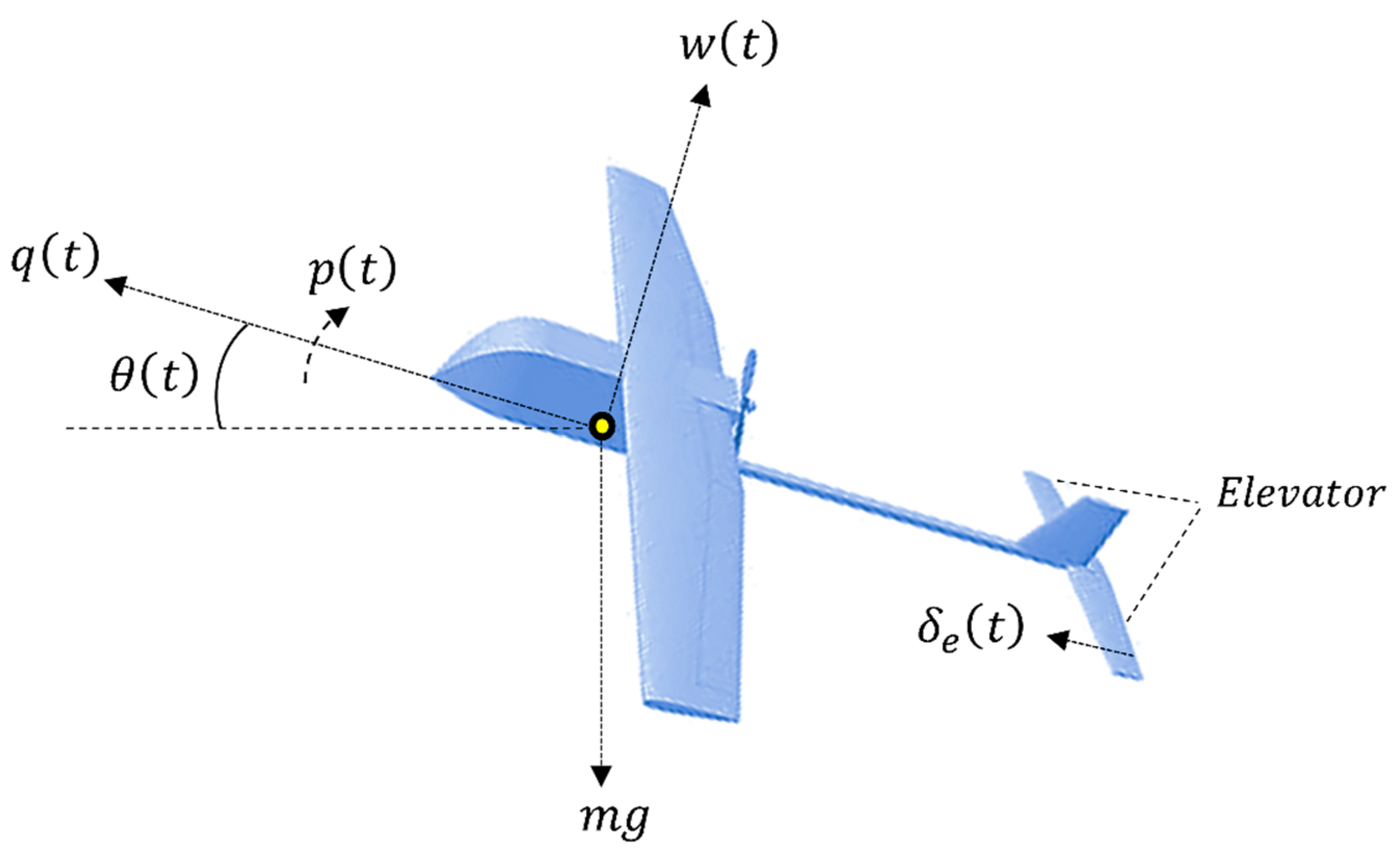
2. System Description

The UAV is a canonical benchmark system chosen for its complex aerodynamics and kinematic instability. The dynamic motion of a UAV is generally classified into four categories: directional, forward, longitudinal, and lateral [29,30]. However, as discussed earlier, this research work focuses solely on the UAV’s longitudinal motion, which is governed by variations in the vehicle’s pitch angle, forward velocity, and altitude [31,32]. To simplify its complex aerodynamic behavior, the nonlinear equations of motion governing the UAV’s longitudinal motion are linearized around a steady-state operating condition. The longitudinal motion dynamics of a small UAV, Bluebird, are considered for the investigation of the proposed control scheme in this study [6]. The UAV is assumed to operate in steady, level flight with a constant velocity. The elevator’s deflection angle is manipulated by appropriately rotating a DC servomotor onboard the UAV.

2.1. State Space Model

The state-space model representing the UAV’s longitudinal motion is expressed in (1) [11,29].
q ˙ t w ˙ t p ˙ t θ ˙ t = X q X w X p g cos θ o Z q Z w Z p   0 M q 0 M w 0 X p   0 1   0 q t w t p t θ t + X δ Z δ M δ 0 δ e t , θ t = 0 0 1 0 q t w t p t θ t + 0 δ e t
where q t is the forward velocity, w t is the vertical velocity, p t is the pitch rate, θ t is the pitch angle, and δ e t represents the elevator’s deflection angle. It is to be noted that p t = θ ˙ t . The coefficients of the system matrix ( X q , X w , X p , Z q , Z w , Z p , M q , M w , and M p ) are denoted as the stability derivatives, while the coefficients of the input matrix ( X δ , Z δ , and M δ ) are denoted as the control derivatives [29]. The parameter g = 9.81   m / s 2 represents the gravitational acceleration, while θ o is the elevator trim. The schematic representing the longitudinal flight dynamics of a UAV is shown in Figure 1. The coefficients of the system matrix and the input matrix are identified by considering the dynamics of the Bluebird UAV, described in [11,30].
Upon the substitution of the model parameter values, expressed in [11,30], the nominal state space model of the UAV system is presented in Equation (2).
q ˙ t w ˙ t p ˙ t θ ˙ t = 0.045 0.183 0 0.241 0.312 1.945 1   0 0.152 0 22.511 0 2.036 0 1   0 q t w t p t θ t + 0.007   0.124 17.105 0 δ e t
The vertical movement of the UAV is categorized into the short-period model and the long-period model. For the purpose of this study, the short-period model is employed as it provides a more accurate representation than the phugoid model [30]. The change in the UAV’s vertical velocity w t and its pitch rate p t   are sufficient to depict the short-period motion. The forward flight speed is practically the same. The dynamics of the vertical motion are simplified if q t = 0 , and consequently, the short-period model is represented as follows [11,30]:
w ˙ t p ˙ t = 1.945   1 22.511 2.036 w t p t +   0.124 17.105 δ e t p ˙ t = 0 1 w t p t + 0 δ e t
The short-period model occurs over a brief period, during which changes in pitch angle are significant. As a result, the pitch rate p t dominates the dynamics, while variations in vertical velocity w t remain relatively small and less significant in practical flight conditions [28]. Since short-period motion primarily consists of rapid pitch oscillations, the influence of w t is negligible compared to p t . Therefore, deriving the transfer function solely in terms of p t simplifies the system without compromising essential dynamic behavior [11,30]. Thus, the state-space model in Equation (3) is used to derive the system’s transfer function from the elevator’s deflection angle to the UAV’s pitch rate. It is expressed in Equation (4).
p s δ e s = 17.11 s 36.06 s 2 + 3.98 s + 26.47
where s is the Laplace operator. The transfer function representing the UAV’s steering inertia model (elevator model) is expressed as follows [30]:
δ e s v s = K s τ s + 1
where v s is the control input voltage applied to the elevator’s servomotor, K s is the servomotor’s gain constant, and τ is the servomotor’s time constant. As discussed in the previous studies, the values of K s and τ are set at 1 and 0.1 s, respectively, for the Bluebird UAV [11,30]. The resulting transfer function depicting the relationship between the elevator’s servo control input v s and the UAV’s pitch angle θ s is derived in the following expression.
p s v s = 171.1 s + 360.6 s 3 + 13.98 s 2 + 66.28 s + 264.7
The aforementioned transfer function is converted into the system’s corresponding state space model. For this purpose, the transfer function is dissociated into two separate blocks, as shown below.
m s v s = 1 s 3 + 13.98 s 2 + 66.28 s + 264.7 ,   p s m s = 171.1 s + 360.6  
The variable m t and its higher-order derivatives are chosen as the intermittent state variables of the system, relating the servomotor’s rotation to the UAV’s pitch angle. The expressions in Equation (8) are transformed into the time domain as shown below.
m t + 13.98 m ¨ t + 66.28 m ˙ t + 264.7 m t = v t  
p t = 171.1 m ˙ t + 360.6 m t
To improve the UAV’s longitudinal reference tracking accuracy and robustness against bounded perturbations, a supplementary pitch-rate-error integral variable ε t , expressed in (10), is also included in the system’s mathematical model [33].
ε t = e p t d t  
s u c h t h a t ,   e p t = θ ˙ r θ ˙ t
where θ ˙ r is the reference pitch rate of the UAV, and e p t is the error between the reference and the actual pitch rates of the UAV. The error integral variable is rewritten as follows:
ε ˙ t = θ ˙ r θ ˙ t
Since p t = θ ˙ t ; therefore, by substituting Equation (9) in the above equation, the following expression is derived.
ε ˙ t = θ ˙ r 171.1 m ˙ t 360.6 m t
The state space model of a linear dynamical system is expressed as shown below.
x ˙ t = A x t + B u t + G r t ,   y t = C x t + D u t  
where x t is the state vector, y t is the output vector, u t is the voltage input, r t is the reference pitch rate, A is the system matrix, B is the control input matrix, G is the reference input matrix, C is the output matrix, and D is the feed-forward matrix. The state, input, reference pitch, and output variables of the said UAV system are expressed as Equation (14).
x t = m t m ˙ t m ¨ t ε ˙ t T ,   u t = v t ,   r t = θ ˙ r ,   y t = p t
The state space matrices of Bluebird’s UAV model are expressed in (15).
A = 0 1 0   0 0 0 1   0 264.7 360.6 66.28 171.7 13.98 0 0   0 ,   B = 0 0 1 0 ,   G = 0 0 0 1 , C = 360.6 171.1 0 0 ,   D = 0

2.2. Baseline LQI Controller

The Linear Quadratic Integral (LQI) controller is a state-feedback compensator that improves the system’s reference tracking accuracy while reducing overshoots and undershoots by introducing an integral error component into the standard LQR framework [33,34]. The control law is formulated by minimizing a quadratic cost function, which penalizes deviations in both system states and control inputs. The cost function is mathematically represented as follows [35]:
J l q i = 1 2 0 x t T Q x t + u t T R u ( t ) d t
The state-weighting matrix Q   4×4 is positive semi-definite, while the control-weighting matrix R   ℝ is positive definite. These matrices are customized to provide a well-balanced compromise between the system’s control effort and reference tracking accuracy. The proposed UAV system’s Q and R matrices are represented in Equation (17).
Q = d i a g q m q m ˙ q m ¨ q ε ˙ , R = p
To acquire an asymptotically stable control law, the coefficients of the Q and R matrices are chosen so that q m 0 , q m ˙ 0 , q m ¨ 0 , q ε 0 , and   p > 0 . Section 4 describes the offline tuning approach used to configure these coefficients. Once the weighting matrices have been configured offline, the Hamilton–Jacobi–Bellman (HJB) equations are solved to obtain the LQI control law. Their solution yields the following algebraic Riccati Equation (ARE) [35].
A T P + P A P B R 1 B T P + Q = 0
The positive definite, symmetric matrix P   4×4 represents the ARE’s solution. The state-compensator gain vector K is computed as described in Equation (19) [35].
K = R 1 B T P
The optimal LQI control law thus derived from solving the ARE is expressed in Equation (20).
u t = K x t
where K = k m k m ˙ k m ¨ k ε ˙ . This integral component enhances the system’s ability to eliminate steady-state errors and improves disturbance rejection.
Stability Proof: The LQI controller’ stability is established via the following Lyapunov function, ensuring asymptotic convergence under appropriate weight selection [33].
Z t = x t T P x t > 0 ,   f o r x t 0
The first derivative of Z t is obtained as illustrated below.
Z ˙ t = 2 x t T P x ˙ t = 2 x t T P A B K x t = 2 x t T P A B R 1 B T P x t = x t T P A + A T P x t 2 x t T P B R 1 B T P x t
Substituting Equation (18) into Equation (22) simplifies Z ˙ t , as expressed below.
Z ˙ t = x t T Q x t x t T P B R 1 B T P x t < 0
The expression in Equation (22) depicts that Z ˙ t becomes a negative definite function if R = R T > 0 and Q = Q T 0 . Hence, fulfilling the aforementioned prerequisites serves to preserve the asymptotic stability of the LQI control law. The schematic of the LQI control architecture used for the UAV’s longitudinal motion control is shown in Figure 2.

3. Proposed Control Methodology

A fixed-gain LQI controller has various drawbacks in UAV longitudinal motion control owing to its inability to adapt to changing flight conditions. Since it operates with fixed state feedback gains, the typical LQI controller has difficulty dealing with wind disturbances, payload variations, and changes in actuator dynamics and other aerodynamic parameters [33]. Parametric uncertainties caused by variations in both payload and actuator dynamics affect key system parameters, modifying the UAV’s dynamics. The fixe-gain LQI controller generally results in suboptimal performance, where high-gain settings result in excessive control effort and actuator saturation, while a low-gain design compromises tracking precision and disturbance rejection. Furthermore, the fixed-gain LQI controller does not dynamically modify its reaction to exogenous disturbances during a given flight phase, resulting in slow response speed, forceful oscillations, overshoots, or even instability since the controller lacks real-time adaptation to overcome unanticipated perturbations. To overcome these limitations, an LCA was investigated in this study.

3.1. Learning Control Algorithm (LCA)

The LCA scheme is formulated by incorporating model-reference tracking, dissipative, and anti-dissipative terms, which allows the control scheme to robustly suppress oscillations in nominal conditions while intensifying control efforts under severe disturbances, ensuring fast yet smooth recovery. The baseline LCA is formulated in Equation (24) [36].
u ˙ t = β u t + γ u t u l q i t + δ e θ t + ρ e θ 3 t sign e ˙ θ t
such that, e θ t = θ r θ t
where θ r is the reference pitch angle of the UAV, and e θ t is the error between the reference and the actual pitch angles of the UAV, u l q i t represents the control effort generated by the LQI control law in (20), β represents the control-decay rate, γ represents the model-reference tracking rates, δ represents the disturbance-rejection rate, and ρ is the predetermined weight of the error cube signal e θ 3 t . These parameters are optimized offline by using the tuning procedure discussed in Section 4. The LCA formulation comprises the three distinct control components presented in Table 1.
The model-reference tracking term is tasked to operate under moderate error conditions. The dissipative and anti-dissipative control terms manipulate the control system’s adaptability under very small error (equilibrium) or very large error (disturbance) conditions, respectively. The following rationale is used to formulate the LCA [36].
The model-reference tracking term assists the LCA to track the baseline LQI controller, u l q i t , which acts as a reference control law under normal operating conditions. By aligning with the LQI baseline, the LCA ensures stability and optimal state regulation in the absence of major disturbances, resulting in smooth system operation and low control effort. Additionally, it also ensures smooth transitions between the dissipative and anti-dissipative terms.
The dissipative component regulates the system’s energy dissipation under small error conditions, ensuring a steady and controlled convergence to equilibrium while avoiding excessive servo control requirements. It exponentially reduces the applied control effort when the system’s response is converging (or settling at) the desired reference or when the anti-dissipative term becomes fragile.
The anti-dissipative component introduces robust corrective actions under large error conditions by appropriately amplifying (or attenuating) the applied control input in response to the system’s error phase under major disturbances, effectively counteracting perturbations and accelerating transient recovery.
The anti-dissipative component is realized by utilizing the error phase information of the system’s state response under exogenous disturbances. Figure 3 illustrates the error profile of an arbitrary system subjected to an external disturbance, highlighting four distinct error phases (A to D) [37]. When the system response deviates from the reference (phases A and C), the product of the state error and its derivative becomes positive, indicating divergence and necessitating a stiff control action. In contrast, the said product becomes negative when the response is converging to the reference (phases B and D), and thus, necessitates a softer control application.
The above rationale is mathematically formulated to define the phase-informed anti-dissipative term, h t , as presented in Equation (25).
h t = e θ t + ρ e θ 3 t sign e ˙ θ t  
where ρ is the predefined weighting coefficient of e θ 3 t . It is optimized offline by using the tuning procedure discussed in Section 4. The signum function, s i g n . , is expressed as follows:
sign e ˙ θ t = 1 , i f   e ˙ θ t > 0 0 , i f   e ˙ θ t = 0 1 , i f   e ˙ θ t < 0
The error cube polynomial e θ t + ρ e θ 3 t in the anti-dissipative term introduces distinct amplified and attenuated error regions, as shown in Figure 4, flexibly adjusting the control response based on error magnitude [38]. It enhances the controller’s responsiveness by intensifying control efforts for large errors, ensuring rapid correction while attenuating control actions for small errors, preventing excessive actuator activity, and minimizing steady-state fluctuations. Consequently, the applied control input exhibits a sharp increase in magnitude under significant error conditions, while maintaining a more conservative response in near-equilibrium states.

3.2. Reconfigurable Learning Control Algorithm (RLCA)

To further improve the system’s adaptability to parametric uncertainties, the aforementioned LCA employs a state-error-driven gain modulation mechanism that regulates the inclusion of dissipative, model reference tracking, and anti-dissipative control terms. The proposed RLCA dynamically reconfigures the weights applied to its constituent control components based on state error variations, ensuring efficient disturbance rejection while preventing excessive control effort.
This arrangement provides a gradual transition between control phases, minimizing chattering and actuator wear. The adaptive weight modulation of the three control terms constituting the LCA is governed by a pre-calibrated hyperbolic secant function (HSF). It dynamically adjusts the weighting of the model-reference tracking, dissipative, and anti-dissipative contributions based on state error magnitudes. The HSF is chosen for its smooth, even-symmetric waveform, which normalizes the input variables within the range of zero to one [38]. The HSF-based adaptive weighting functions are formulated as per the following metarules.
  • For small errors, the adaptation law intensifies the dissipative control action, applying minimal corrective control.
  • For moderate errors, a combination of dissipative and model-reference tracking terms is deployed to ensure optimal state regulation without excessive control input.
  • For large errors, the anti-dissipative term is activated to intensify the (phase-informed) control actions for robust disturbance rejection, followed by a gradual transition back to nominal conditions.
The aforementioned rationale is diagrammatically expressed in Figure 5.
The following HSF-based weighting functions are thus constituted to comply with the aforementioned metarules.
α S t = sech μ   e θ t ,   α L t = 1 α S t ,   α M t = 2 α L t α S t
where sech . represents the HSF, and μ is the preset positive variation rate of the HSF. The waveforms of these hyperbolic gain scaling functions are shown in Figure 6.
The dissipative term is weighted by α S t to direct the control law under small error conditions, the anti-dissipative term is weighted by α L t to direct the control law under large error conditions, and the model-reference tracking term is weighted by α M t to ensure the applied control actions track the nominal LQI trajectory. Parameter μ is optimized offline by using the tuning procedure discussed in Section 4. The proposed RLCA is formulated in Equation (28).
u ˙ t = α S t β u t + α M t γ u t u l q i t + α L t δ e θ t + ρ e θ 3 t sign e ˙ θ t
If u m t = u t u l q i t , the RLCA control law can be rewritten as follows.
u ˙ t = α S t β   u t + α M t γ   u m t + α L t δ   h t
The system continuously refines its control actions based on the formulated algebraic law. This differential equation is numerically integrated at each sampling interval, as shown in Equation (30), to ensure real-time adaptability.
u t = e α S t β t   u 0 + 0 t e α S t β t p α M p γ   u m p + α L p δ   h p d p
The control actions are refined online, after every sampling instant, based on the system’s state and error variations. The control adaptation process begins by utilizing the nominal control signals u 0 generated by the LQI controller. It is to be noted that as long as the power of the exponential term α S t β is negative definite, the term e α S t β t decays to zero as time progresses. To ensure that the power of the exponential term α S t β remains strictly negative, a small offset = 0.01 is added in α S t β , turning it into α S t β + . This arrangement prevents it from reaching zero under every operating condition. The updated control law is shown in Equation (31).
u t = e α S t β + t   u 0 + 0 t e α S t p β + t p α M p γ   u m p + α L p δ   h p d p
This behavior signifies that the system is exponentially stable, as the output diminishes over time. Based on this condition, the finalized RLCA control law is presented in Equation (32).
u ˙ t = α S t β +   u t + α M t γ   u m t + α L t δ   h t
Under nominal conditions, the system remains stable as it tracks the LQI controller, whose asymptotic stability has been rigorously established in the preceding section. To prevent the actuator from saturation under large servo requirements caused by external disturbances, the control signal u t is bounded between 0 and 10 V, by using the saturation function of the following form.
10   s a t u t = 10   V ,   u t > 10   V u t ,   0 u t 10   V   0 ,   u t < 0
The combination of these terms allows the controller to dynamically adjust damping stiffness and response speed in reaction to disturbances while maintaining closed-loop stability. The RLCA updates the weighting of the three control terms constituting the LCA, solving the algebraic equations (for adaptive weight modulation) numerically at each sampling interval. This self-learning approach strengthens the UAV’s damping control strength and improves its transient recovery speed against external disturbances during the longitudinal motion. The schematic of the RLCA law designed for UAV’s longitudinal motion control, as per the formulations in Equations (27) and (28), is shown in Figure 7.

4. Parameter Optimization Procedure

This section describes the tuning procedure used to offline optimize the coefficients of the state and control-weighting matrices, expressed in Equation (17), associated with the baseline LQI controller as well as the learning parameters ( β , γ , δ , ρ , and μ ) linked with the RLCA scheme. The optimization is carried out by minimizing the cost function in Equation (34).
J e = 0 T e θ t 2 + u t 2 d t
where T is the total duration of a simulation trial. The said cost function captures the variations in the system’s state error e θ t as well as the applied control input u t . The function assigns equal weights to both variables to optimize state regulation while economizing the control energy expenditure. The coefficients of the state and control-weighting matrices of the LQI controller are chosen within the range of 0 to 100. The parameters associated with the RLCA are chosen within the range of 0 and 10. Section 5 outlines the procedure for conducting simulation trials to tune the parameters. All tuning parameters are initially set to unity. Figure 8 illustrates the parameter tuning process [33].
The tuning begins with initial parameter settings and proceeds iteratively [37]. In each trial, the UAV model is tasked to track a step reference position along the longitudinal axis for T = 5.0 s, during which the cost J e , k is evaluated; where k is the trial number. The algorithm searches for optimal parameters by following the descending gradient of the cost function. If a new trial results in a lower cost J e , k than the cost of the previous trial J e , k 1 , the local minimum J e , m i n is updated. The process stops when either the maximum number of trials ( k m a x ) is reached or the cost falls below a predefined threshold. This threshold is determined empirically through pilot runs, ensuring a balance between computational efficiency and solution accuracy while preventing premature termination. To determine the said threshold, the cost for the initial parameter settings is recorded as J e , m i n 0 2.47 × 10 4 , and its scaled-down value (heuristically set to 0.05) is used as the algorithm termination criterion. A larger scaling factor increases computational demands, while a smaller one risks premature termination. The algorithm is thus concluded when J e , m i n approaches 0.05   J e , m i n 0 .
Accordingly, the threshold value for J e , m i n as well as k m a x are set at 1.2 × 10 3 and 40, respectively. Thus, the state and control costs optimized are Q = d i a g 1.05 31.58 3.22 2.11 and R = 1.02 , respectively. Correspondingly, the LQI state feedback gain vector is computed as K = 0.66 5.34 3.41 1.85 . Similarly, the optimized values of the parameters linked with the RLCA scheme are β = 4.092 , γ = 3.87 , δ = 5.63 , ρ = 1.48 , and μ = 2.19 .

5. Simulations and Results

This research adopts a phased approach, with successful simulation results serving as a foundation for further experimental validation. Given the preliminary nature of this investigative study, meticulous simulations are required to evaluate the proposed controller’s effectiveness and reliability. They allow for repeated refining and optimization, resulting in a well-validated framework before moving on to resource-intensive hardware-in-the-loop experiments, improving the likelihood of success in subsequent stages. Hence, this section presents the test simulations along with a thorough comparative analysis of the aforementioned longitudinal motion control techniques for a UAV to ensure their optimality and resilience in the time-domain.

5.1. Simulation Setup

The reference tracking performance of the LQI controller and the proposed RLCA are evaluated in the time domain through customized simulations under nominal conditions, sudden wind gusts, constant wind disturbance, cruise altitude adjustments, and aerodynamics parameter variations. The control application is implemented in MATLAB/Simulink R2020b and executed on a 64-bit embedded computer (2.1 GHz CPU, 12 GB RAM). The sampling frequency is set at 250 Hz. As outlined in Section 2, the longitudinal motion dynamics of a small UAV, Bluebird, are considered to validate the proposed controller’s effectiveness in tracking the reference trajectory while rejecting the bounded exogenous disturbances. The band-limited white noise is incorporated into the control input to simulate the effects of moderate turbulence and typical sensor noise encountered in UAV operations. In MATLAB/Simulink, the said noise block is configured with a noise power of 10−3 and a sampling time of 4.0 msec., ensuring a realistic representation of sensor disturbances in the system. To prevent the elevator’s actuator saturation, the control input signal u t is restricted between 0 and 10 V.

5.2. Simulation Results

Five testing scenarios were used to benchmark the proposed RLCA against the LQI controller. Simulations evaluated each controller’s performance individually for the UAV model being considered. The closed-loop system ensures continuous tracking of the UAV’s longitudinal position reference, under every operating condition. In each case, an additive white Gaussian noise signal was introduced in the system’s reference input to emulate the impact of sensor noise in real-time flight scenarios.
A.
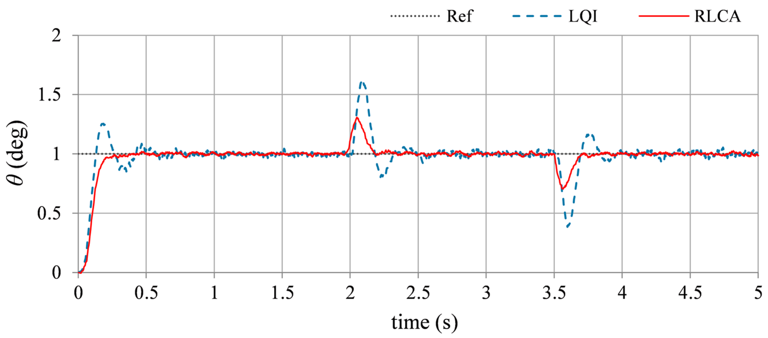
Step reference tracking: This simulation case is used to evaluate the controller’s ability to track step changes in altitude under nominal (disturbance-free) conditions. The UAV longitudinal model with nominal parameters is used. The test is performed by tasking the UAV to track a step reference trajectory of +1.0 deg. The variations in the pitch angle of the LQI controller and the RLCA are shown in Figure 9.
B.
Ramp reference tracking: This test case assesses the UAV’s ability to follow continuously changing altitude as a result of cruise altitude adjustments for steady ascent (or descent) during long-range flights. A ramp trajectory closely mimics how a UAV’s autopilot system adjusts altitude smoothly during the takeoff phase or the landing phase. Hence, this test is performed by tasking the UAV model to track the ramp reference trajectory of 4.0 deg. peak-to-peak amplitude, +3.0 deg. offset, and a frequency of 0.1 Hz to represent a gradual altitude climb and descent. The reference tracking accuracy (or lag) manifested by each controller is presented in Figure 10.
C.
Impulsive disturbance suppression: This simulation is used to test the UAV’s disturbance rejection ability against sudden external forces caused by wind gusts or mid-air collision with flying objects. The test is performed by introducing an external pulse of ±2.0 V magnitude and 100 ms duration in the control input signal at t = 2.0 s and t = 3.5 s, respectively, to observe the system’s transient response. This arrangement emulates the application of a short-duration impulsive force under steady flight conditions of the UAV. The time domain profiles of the UAV’s pitch angle, under the influence of each controller, are shown in Figure 11.
D.
Step disturbance rejection: This simulation case examines the UAV’s response to sustained external disturbances, such as constant wind disturbance or a sudden change in elevator deflection. The test is performed by introducing an external step signal of +1.0 V magnitude and 100 ms duration in the control input signal at t = 2.0 s to observe the system’s disturbance recovery response. This arrangement emulates the application of a constant external force under steady flight conditions of the UAV. The time domain profiles of the UAV’s pitch angle, under the influence of each controller, are shown in Figure 12.
E.
Model uncertainties compensation: This simulation evaluates the UAV’s ability to compensate for model uncertainties resulting from variations in actuator dynamics. This scenario captures a critical aspect of uncertainty compensation—adjustments in control system dynamics due to actuator nonlinearities or miscalibrations. The test is conducted by increasing the servomotor gain K s by 20% at t = 2.0 s, simulating the actuator’s sensitivity to hardware inconsistencies or miscalibrations. The sudden increment in K s modifies the UAV’s state-space model by changing key system parameters, and altering the elevator’s control response characteristics, which potentially affects the UAV’s pitch stability and tracking accuracy. The time-domain responses of the UAV’s pitch angle, under the influence of each controller, are presented in Figure 13.
F.
Performance under extreme conditions: To rigorously assess the robustness of the UAV’s control algorithm in extreme real-world conditions, a test case is designed with simultaneous dynamic variations, external disturbances, and sensor noise. The UAV follows a continuous ramp reference trajectory, challenging its tracking performance under changing setpoints. Sudden impulsive disturbances of ±2.0 V magnitude and 100 ms duration are injected at discrete intervals to simulate wind gusts or mid-air collisions, while band-limited white noise is added to the control input to replicate turbulence and sensor noise. Additionally, a 20% increment in the UAV’s servomotor gain K s at t ≈ 8.0 s is introduced to assess robustness against model-induced parametric uncertainties. The time-domain responses of the UAV’s pitch angle, under the influence of each controller, are presented in Figure 14.

5.3. Performance Evaluation and Discussion

The simulation results are assessed using the following key performance metrics (KPMs).
  • RMSEθ: The root mean squared value of the tracking error e θ , calculated as follows:
    R M S E θ = e θ n 2 n
    where n represents the total number of samples.
  • OS: The peak deviation observed during the start-up phase of the response;
  • Tset: The duration required for the system response to settle within ±2% of the reference value;
  • Mpeak: The maximum deviation (overshoot or undershoot) that occurs following a disturbance;
  • Trec: The time taken for the response to stabilize within ±2% of the reference value after experiencing a disturbance.
Table 2 presents a quantitative summary of the simulation results, demonstrating the robust tracking and disturbance rejection capabilities of the proposed control law. The results validate that the proposed RLCA robustifies control performance by ensuring a balanced trade-off between aggressive and conservative control actions, improving transient response, and preserving steady-state accuracy.
In Test A (Figure 9), the LQI controller exhibits moderate tracking performance, characterized by noticeable overshoot, oscillations, and an extended settling time. In contrast, the RLCA scheme achieves superior tracking accuracy, with minimal overshoot, faster convergence, and reduced steady-state fluctuations. In Test B (Figure 10), the LQI controller maintains an oscillatory tracking response and demonstrates sensitivity to sinusoidal disturbance, resulting in lag and noticeable degradation in tracking accuracy. Meanwhile, the RLCA scheme exhibits greater robustness and adaptability to track the ramp trajectory, while also optimizing control resource allocation. In Test C (Figure 11), the LQI-controlled system shows noticeable deviations from the reference trajectory, followed by a slow recovery. In contrast, the RLCA scheme effectively dampens impulsive disturbances, quickly restoring the system to its reference position while also attenuating peak overshoots. In Test D (Figure 12), the LQI controller struggles to maintain steady-state accuracy after a disturbance and exhibits a slower transient recovery. However, the RLCA scheme achieves superior trajectory tracking accuracy by efficiently adapting to the step disturbance. In Test E (Figure 13), the LQI controller demonstrates poor model error compensation, with large fluctuations in the response. Conversely, the RLCA scheme significantly improves disturbance attenuation, resulting in a smoother response. Similarly to payload variations, the changes in actuator dynamics also impact the UAV’s state-space model by modifying key system parameters. While actuator variations alter control effectiveness, payload changes affect stability derivatives. However, both of these parametric uncertainties influence the UAV’s overall flight behavior. Since both scenarios lead to variations in UAV’s system dynamics, the outcomes of Test E validate that RLCA’s adaptive control strategy remains effective in compensating for such uncertainties in real time.
In Test F (Figure 14), the LQI controller exhibits noticeable chattering and sensitivity to disturbances in the tracking response, leading to increased tracking error and slower stabilization. Specifically, it demonstrates higher RMSEθ, peak deviations, and recovery times, resulting in lag and reduced accuracy. Meanwhile, the RLCA scheme significantly enhances robustness and adaptability, effectively minimizing tracking error, overshoot, and transient recovery time. By adaptively regulating the control resource allocation, the RLCA scheme ensures improved disturbance rejection and faster transient recovery, making it a superior alternative to the LQI controller.
The superior performance of the RLCA over the LQI controller is attributed to its adaptive gain modulation and structured control strategy. Unlike the fixed-gain LQI, which applies uniform control gains irrespective of varying system conditions, the RLCA dynamically adjusts its control response based on real-time state errors. This adaptability enables it to achieve improved tracking accuracy, faster convergence, and better disturbance rejection. One of the primary advantages of the RLCA is its ability to effectively mitigate overshoot while enhancing convergence speed. This is achieved through the interplay of its three constituent control terms:
  • Dissipative control component: Under small error conditions, the dissipative term ensures controlled energy dissipation, preventing excessive control input fluctuations that could lead to oscillations or overshoot. This mechanism exponentially attenuates the applied control action as the system state approaches equilibrium, ensuring a smooth and stable convergence.
  • Model-reference tracking component: The RLCA employs an LQI-derived model-reference tracking term, which acts as a baseline controller under nominal conditions. By maintaining alignment with the LQI control law when disturbances are absent, the RLCA preserves steady-state accuracy while minimizing unnecessary control effort. This ensures that the system operates optimally without excessive control actions that could compromise stability.
  • Anti-dissipative control component: In contrast to the LQI controller, which lacks a real-time adaptive response to exogenous perturbations, the RLCA leverages an anti-dissipative term informed by the phase of the system’s state error. This term intensifies control actions under large error conditions, ensuring rapid disturbance rejection. The inclusion of an error cube polynomial further amplifies corrective control inputs when the system deviates significantly from the reference trajectory, accelerating transient recovery while maintaining stability.
These control components are self-regulated via HSF-based adaptive weight functions, allowing smooth transitions between different control phases while minimizing chattering and actuator stress. By dynamically modulating control gains in response to real-time system states, the RLCA achieves an optimal balance between aggressive correction during disturbances and conservative control near equilibrium, which accounts for its reduced overshoot and faster convergence speed. The synergistic combination of the aforementioned three control actions enhances the controller’s adaptability by enabling it to flexibly manipulate the control trajectory as per the state error variations.
These theoretical insights are corroborated by the simulation results, where the RLCA consistently demonstrates lower RMSEθ values, reduced peak deviations, and shorter settling times across multiple test scenarios, including nominal tracking, impulsive disturbances, and model uncertainties. This highlights the RLCA’s robustness and adaptability, making it a more effective solution for UAV longitudinal motion control compared to the fixed-gain LQI controller.

6. Conclusions

This study presents the methodical formulation of an innovative RLCA framework for robust optimal longitudinal motion control of UAVs, enhancing its trajectory tracking precision and disturbance rejection capacity. The baseline elevator position control procedure is realized by implementing a fixed-gain LQI tracking control law. However, the baseline LQI controller is limited by its inability to adapt to disturbances and changing flight conditions, resulting in either excessive control effort or poor tracking performance. Therefore, the baseline control procedure is supplemented by augmenting it with a learning-based adaptative control law that employs self-adjusting dissipative, anti-dissipative, and model-reference tracking control terms. The resulting RLCA scheme dynamically modulates its learning gains, ensuring robust disturbance rejection, smoother transitions, reduced control energy consumption, and enhanced stability during the vertical (longitudinal) flight phase of the UAV. By dynamically balancing aggressiveness and conservatism in control actions, the RLCA effectively reduces overshoot, enhances convergence speed, and ensures robust trajectory tracking, making it a more reliable choice for UAV longitudinal motion control. The proposed control algorithm is benchmarked against the baseline LQI controller by performing credible MATLAB simulations. The simulation results verify that the structured adaptability allows the RLCA to outperform the traditional LQI control in managing the UAV’s longitudinal motion under bounded exogenous disturbances.
Several potential research directions can be explored in the future to further enhance the robustness of the proposed RLCA for UAV longitudinal motion control. The effectiveness of the RLCA framework can be further validated through hardware-in-the-loop flight experiments to assess its practical feasibility under real aerodynamic conditions and actuator constraints. The hyperbolic gain scaling mechanism of the learning gains can be replaced by fuzzy inference systems, neural networks, or other computational intelligence algorithms. To validate the RLCA’s adaptability to payload variations, tailored simulations can be conducted that involve variations in the system’s stability derivatives to alter the UAV’s mass distribution. Finally, the proposed controller design can be extended by employing data-driven and reinforcement-learning-based schemes to analyze the system’s adaptability, practicality, and computational complexity in real-time applications.

Author Contributions

Conceptualization, O.S.; methodology, O.S.; software, O.S. and A.T.; validation, J.I.; formal analysis, O.S. and A.T.; investigation, A.T.; resources, J.I.; data curation, A.T.; writing—original draft preparation, O.S.; writing—review and editing, J.I.; visualization, A.T.; supervision, J.I.; project administration, J.I. All authors have read and agreed to the published version of the manuscript.

Funding

This research received no external funding.

Data Availability Statement

The data supporting the conclusions of this article will be made available by the corresponding author on a reasonable request.

Conflicts of Interest

The authors declare no conflicts of interest.

References

  1. Irfan, S.; Zhao, L.; Ullah, S.; Javaid, U.; Iqbal, J. Differentiator- and observer-based feedback linearized advanced nonlinear control strategies for an unmanned aerial vehicle system. Drones 2024, 8, 527. [Google Scholar] [CrossRef]
  2. Sonugür, G. A Review of quadrotor UAV: Control and SLAM methodologies ranging from conventional to innovative approaches. Robot. Auton. Syst. 2023, 161, 104342. [Google Scholar]
  3. Asadzadeh, S.; de Oliveira, W.J.; de Souza Filho, C.R. UAV-based remote sensing for the petroleum industry and environmental monitoring: State-of-the-art and perspectives. J. Petroleum Sci. Eng. 2022, 208, 109633. [Google Scholar]
  4. Li, H.; Wang, C.; Yuan, S.; Zhu, H.; Li, B.; Liu, Y.; Sun, L. Energy Scheduling of Hydrogen Hybrid UAV Based on Model Predictive Control and Deep Deterministic Policy Gradient Algorithm. Algorithms 2025, 18, 80. [Google Scholar] [CrossRef]
  5. Tutsoy, O.; Hendoustani, D.; Ahmadi, K.; Nabavi, Y.; Iqbal, J. Minimum distance and minimum time optimal path planning with bioinspired machine learning algorithms for impaired unmanned air vehicles. IEEE Trans. Intell. Transp. Syst. 2024, 25, 9069–9077. [Google Scholar]
  6. Liu, C.; Chen, W. Disturbance Rejection Flight Control for Small Fixed-Wing Unmanned Aerial Vehicles. J. Guid. Control Dyn. 2016, 39, 2810–2819. [Google Scholar]
  7. Ducard, G.; Carughi, G. Neural Network Design and Training for Longitudinal Flight Control of a Tilt-Rotor Hybrid Vertical Takeoff and Landing Unmanned Aerial Vehicle. Drones 2024, 8, 727. [Google Scholar] [CrossRef]
  8. Yang, Y.; Kim, S.; Lee, K.; Leeghim, H. Disturbance Robust Attitude Stabilization of Multirotors with Control Moment Gyros. Sensors 2024, 24, 8212. [Google Scholar] [CrossRef] [PubMed]
  9. Bianchi, D.; Di Gennaro, S.; Di Ferdinando, M.; Acosta Lùa, C. Robust Control of UAV with Disturbances and Uncertainty Estimation. Machines 2023, 11, 352. [Google Scholar] [CrossRef]
  10. Yit, K.K.; Rajendran, P. Enhanced Longitudinal Motion Control of UAV Simulation by Using P-LQR Method. Int. J. Micro Air Vehicle 2015, 7, 203–210. [Google Scholar] [CrossRef]
  11. Li, J.; Liu, X.; Wu, D.; Pi, Z.; Liu, T. A High Performance Nonlinear Longitudinal Controller for Fixed-Wing UAVs Based on Fuzzy-Guaranteed Cost Control. Drones 2024, 8, 661. [Google Scholar] [CrossRef]
  12. Sree Ezhil, V.R.; Rangesh Sriram, B.S.; Christopher Vijay, R.; Yeshwant, S.; Sabareesh, R.K.; Dakkshesh, G.; Raffik, R. Investigation on PID controller usage on Unmanned Aerial Vehicle for stability control. Mater. Today: Proc. 2022, 66, 1313–1318. [Google Scholar] [CrossRef]
  13. Nguyen, D.H.; Lowenberg, M.H.; Neild, S.A. Identifying limits of linear control design validity in nonlinear systems: A continuation-based approach. Nonlinear Dyn. 2021, 104, 901–921. [Google Scholar] [CrossRef]
  14. Saleem, O.; Rizwan, M.; Zeb, A.A.; Ali, A.H.; Saleem, M.A. Online adaptive PID tracking control of an aero-pendulum using PSO-scaled fuzzy gain adjustment mechanism. Soft Comput. 2020, 24, 10629–10643. [Google Scholar]
  15. Zhang, Y.; Zhang, Y.; Zhang, Y. A Fast-Convergent Hyperbolic Tangent PSO Algorithm for UAVs. IEEE Access 2020, 8, 132456–132465. [Google Scholar]
  16. Wang, J.; Zhang, L.; Liu, Y. Parameter Adaptation-Based Ant Colony Optimization with Dynamic Hybrid Mechanism. Int. J. Comput. Intell. Appl. 2020, 19, 215–230. [Google Scholar]
  17. Zhang, L.; Wang, X.; Li, Y. Application of Hybrid Algorithm Based on Ant Colony Optimization and Particle Swarm Optimization in UAV Path Planning. J. Intell. Robot. Syst. 2023, 101, 635–648. [Google Scholar]
  18. Perrusquía, A.; Yu, W. dentification and optimal control of nonlinear systems using recurrent neural networks and reinforcement learning: An overview. Neurocomput 2021, 438, 145–154. [Google Scholar]
  19. Wang, H.; Xu, K.; Liu, P.X.; Qiao, J. Adaptive Fuzzy Fast Finite-Time Dynamic Surface Tracking Control for Nonlinear Systems. IEEE Trans. Circuit Syst. 2021, 68, 4337–4348. [Google Scholar] [CrossRef]
  20. Moali, O.; Mezghani, D.; Mami, A.; Oussar, A.; Nemra, A. UAV Trajectory Tracking Using Proportional-Integral-Derivative-Type-2 Fuzzy Logic Controller with Genetic Algorithm Parameter Tuning. Sensors 2024, 24, 6678. [Google Scholar] [CrossRef]
  21. Kuang, J.; Chen, M. Adaptive Sliding Mode Control for Trajectory Tracking of Quadrotor Unmanned Aerial Vehicles Under Input Saturation and Disturbances. Drones 2024, 8, 614. [Google Scholar] [CrossRef]
  22. Tian, W.; Zhang, X.; Yang, D. Double-layer fuzzy adaptive NMPC coordinated control method of energy management and trajectory tracking for hybrid electric fixed wing UAVs. Int. J. Hydrogen Energy 2022, 47, 39239–39254. [Google Scholar]
  23. Kanokmedhakul, Y.; Bureerat, S.; Panagant, N.; Radpukdee, T.; Pholdee, N.; Yildiz, A.R. Metaheuristic-assisted complex H-infinity flight control tuning for the Hawkeye unmanned aerial vehicle: A comparative study. Expert. Syst. Appl. 2024, 248, 123428. [Google Scholar]
  24. Yanez-Badillo, H.; Beltran-Carbajal, F.; Tapia-Olvera, R.; Favela-Contreras, A.; Sotelo, C.; Sotelo, D. Adaptive robust motion control of quadrotor systems using artificial neural networks and particle swarm optimization. Mathematics 2021, 9, 2367. [Google Scholar] [CrossRef]
  25. Flores, G. Longitudinal modeling and control for the convertible unmanned aerial vehicle: Theory and experiments. ISA Trans. 2022, 122, 312–335. [Google Scholar] [PubMed]
  26. Madeiras, J.; Cardeira, C.; Oliveira, P.; Batista, P.; Silvestre, C. Saturated Trajectory Tracking Controller in the Body-Frame for Quadrotors. Drones 2024, 8, 163. [Google Scholar] [CrossRef]
  27. Liang, X.; Zheng, M.; Zhang, F. A Scalable Model-Based Learning Algorithm with Application to UAVs. IEEE Control Syst. Lett. 2018, 2, 839–844. [Google Scholar] [CrossRef]
  28. Lwin, N.; Tun, H.M. Implementation of flight control system based on Kalman and PID controller for UAV. Int. J. Sci. Technol. Res. 2014, 3, 309–312. [Google Scholar]
  29. Rahimi, M.R.; Hajighasemi, S.; Sanaei, D. Designing and simulation for vertical moving control of UAV system using PID, LQR and Fuzzy Logic. Int. J. Elect. Comput. Eng. 2013, 3, 651. [Google Scholar]
  30. Zhao, X.; Yuan, M.; Cheng, P.; Xin, L.; Yao, L. Robust H∞/S-plane Controller of Longitudinal Control for UAVs. IEEE Access 2019, 7, 91367–91374. [Google Scholar]
  31. Maqsood, A.; Hiong Go, T. Longitudinal flight dynamic analysis of an agile UAV. Aircr. Eng. Aerosp. Technol. 2010, 82, 288–295. [Google Scholar]
  32. Saleem, O.; Kazim, M.; Iqbal, J. Robust Position Control of VTOL UAVs Using a Linear Quadratic Rate-Varying Integral Tracker: Design and Validation. Drones 2025, 9, 73. [Google Scholar] [CrossRef]
  33. Saleem, O.; Iqbal, J. Blood-glucose regulator design for diabetics based on LQIR-driven Sliding-Mode-Controller with self-adaptive reaching law. PLoS ONE 2024, 19, e0314479. [Google Scholar]
  34. Lewis, F.L.; Vrabie, D.; Syrmos, V.L. Optimal Control, 3rd ed.; John Wiley & Sons: Hoboken, NJ, USA, 2012. [Google Scholar]
  35. Saleem, O.; Iqbal, J.; Afzal, M.S. A robust variable-structure LQI controller for under-actuated systems via flexible online adaptation of performance-index weights. PLoS ONE 2023, 18, e0283079. [Google Scholar]
  36. Saleem, O.; Iqbal, J. Phase-Based Adaptive Fractional LQR for Inverted-Pendulum-Type Robots: Formulation and Verification. IEEE Access 2024, 12, 93185–93196. [Google Scholar]
  37. Alagoz, B.B.; Ates, A.; Yeroglu, C.; Senol, B. An experimental investigation for error-cube PID control. Trans. Inst. Meas. Control 2015, 37, 652–660. [Google Scholar]
  38. Hassan, M.A.; Cao, Z.; Man, Z. Hyperbolic-Secant-Function-Based Fast Sliding Mode Control for Pantograph Robots. Machines 2023, 11, 941. [Google Scholar] [CrossRef]
Figure 1. Schematic of the UAV’s longitudinal flight dynamics.
Algorithms 18 00180 g001
Figure 2. Schematic of LQI control law for UAV’s longitudinal motion control.
Algorithms 18 00180 g002
Figure 3. Error profile of a system under disturbance [37].
Algorithms 18 00180 g003
Figure 4. Variation pattern of the error cube polynomial with respect to error variations.
Algorithms 18 00180 g004
Figure 5. Rationale of the proposed RLCA framework.
Algorithms 18 00180 g005
Figure 6. Waveforms of the hyperbolic gain scaling functions expressed in (27).
Algorithms 18 00180 g006
Figure 7. Schematic of RLCA framework for UAV’s longitudinal motion control.
Algorithms 18 00180 g007
Figure 8. Flow of the parameter optimization procedure [33].
Algorithms 18 00180 g008
Figure 9. Step reference tracking response of the UAV under nominal conditions.
Algorithms 18 00180 g009
Figure 10. Ramp reference tracking response of the UAV under nominal conditions.
Algorithms 18 00180 g010
Figure 11. Step reference tracking response of the UAV under impulsive disturbances.
Algorithms 18 00180 g011
Figure 12. Step reference tracking response of the UAV under step disturbance.
Algorithms 18 00180 g012
Figure 13. Step reference tracking response of the UAV under model uncertainties.
Algorithms 18 00180 g013
Figure 14. Ramp reference tracking response of the UAV under impulsive disturbances.
Algorithms 18 00180 g014
Table 1. Description of constituent terms in the control law.
Control TermMathematical Expression
Dissipative term β   u t
Model-reference tracking term γ u t u l q i t
Anti-dissipative term δ e θ t + ρ e θ 3 t sign e ˙ θ t
Table 2. Summary of experimental results.
ExperimentPerformance IndexControl Procedure
SymbolUnitLQIRLCA
ARMSEθdeg.0.0170.013
OSdeg.0.2460.027
Tsetsec.0.5160.296
BRMSEθdeg.0.1270.026
OSdeg.1.5370.217
Tsetsec.0.5140.288
CRMSEθdeg.0.0270.019
OSdeg.0.2550.020
Tsetsec.0.5240.252
Mpeakdeg.0.630.31
Trecsec.0.3050.211
DRMSEθdeg.0.0230.017
OSdeg.0.2470.025
Tsetsec.0.5200.204
Mpeakdeg.0.3330.145
Trecsec.1.2920.815
ERMSEθdeg.0.0280.015
OSdeg.0.2500.010
Tsetsec.0.5170.288
Mpeakdeg.0.7350.270
Trecsec.0.4270.403
FRMSEθdeg.0.2630.081
OSdeg.1.1930.046
Tsetsec.0.4960.302
Mpeakdeg.2.9581.709
Trecsec.0.3440.235
Disclaimer/Publisher’s Note: The statements, opinions and data contained in all publications are solely those of the individual author(s) and contributor(s) and not of MDPI and/or the editor(s). MDPI and/or the editor(s) disclaim responsibility for any injury to people or property resulting from any ideas, methods, instructions or products referred to in the content.

