
Explainable MRI-Based Ensemble Learnable Architecture for Alzheimer’s Disease Detection

 , , , ,
  and
and 
Abstract
:1. Introduction
- This study integrates perturbation-based (LIME) and gradient-based (Saliency and Grad-CAM) interpretability approaches to visualize and explain an ensemble framework consisting of stacking and hard voting techniques, enhancing Alzheimer’s disease diagnosis through magnetic resonance imaging (MRI).
- A comprehensive ensemble architecture is developed that integrates multi-classifier Convolutional Neural Network architectures: VGG-19 for deep feature extraction, ResNet to address vanishing gradients, MobileNet and EfficientNet for efficient processing, DenseNet for feature reuse, a custom multi-classifier CNN, and a Vision Transformer for capturing complex spatial relationships.
- The proposed framework overcomes the limitations of single-model approaches, achieving high diagnostic accuracy and robustness while providing transparent decision-making processes.
- The implemented visualization techniques highlight critical MRI regions, enhancing clinicians’ understanding of the model and making the decision-making process more transparent and trustworthy.
- Experimental results demonstrate that both stacking and hard voting provide a refined focus on diagnostically relevant areas, proving particularly sensitive to early-stage cognitive changes in MCI cases.
2. Related Work
2.1. Perturbation-Based Methods for Explaining Medical Disease Diagnostic and Predictive Models
2.2. Gradient-Based Methods for Explaining Medical Disease Diagnostic and Predictive Models
3. Methodology
| Algorithm 1 A step-by-step XAI workflow for Alzheimer’s Disease detection |
|
3.1. Model Development
| Algorithm 2 CNN architecture for MRI classification |
|
| Algorithm 3 Comprehensive transfer learning architecture for MRI classification |
|
| Algorithm 4 Vision Transformer (ViT) for MRI classification |
|
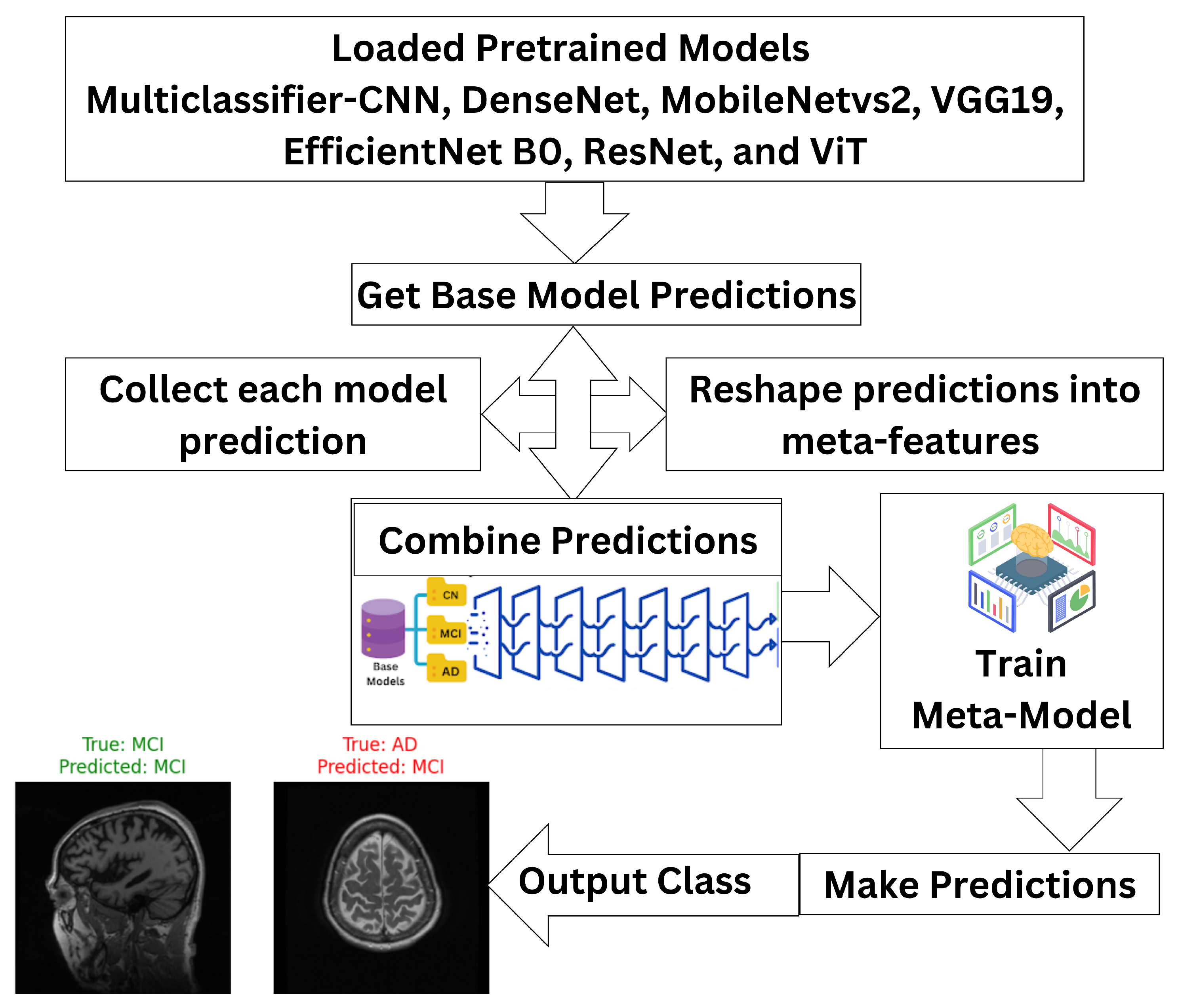
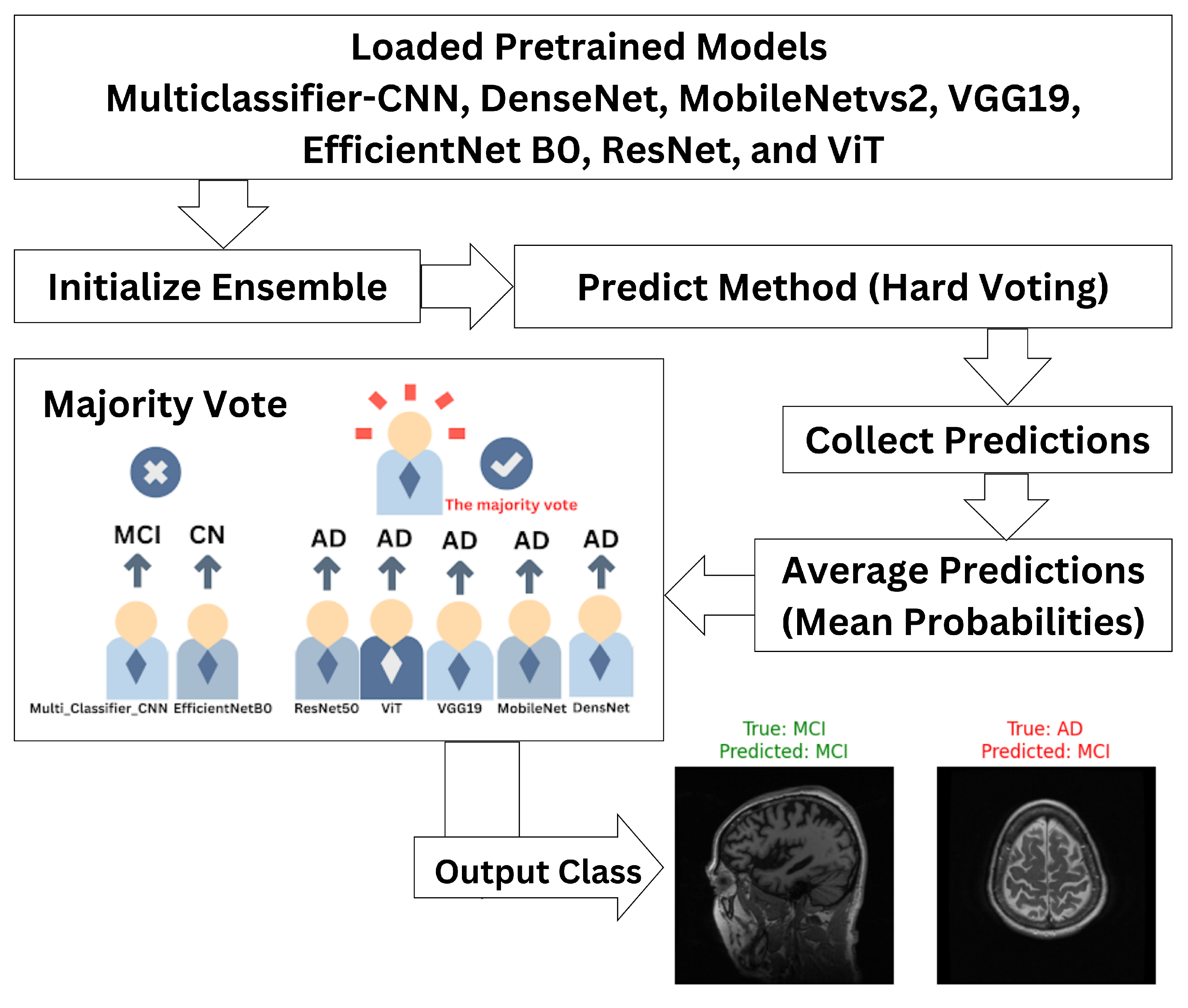
3.2. Ensemble Classifier
- are the predictions from the base models for an input x;
- g denotes the meta-model that combines these predictions to generate the final output .
- is the final ensemble prediction;
- are predictions made by M classifiers;
- mode represents the majority label among the predictions.
3.3. Model Interpretation
3.4. Model Evaluation
- True Positive (TP): Cases correctly identified as positive (correctly diagnosed with Alzheimer’s);
- True Negative (TN): Cases correctly identified as negative (correctly diagnosed as healthy);
- False Positive (FP): Cases incorrectly identified as positive (healthy subjects misdiagnosed with Alzheimer’s);
- False Negative (FN): Cases incorrectly identified as negative (Alzheimer’s subjects misdiagnosed as healthy).
4. Results and Discussion
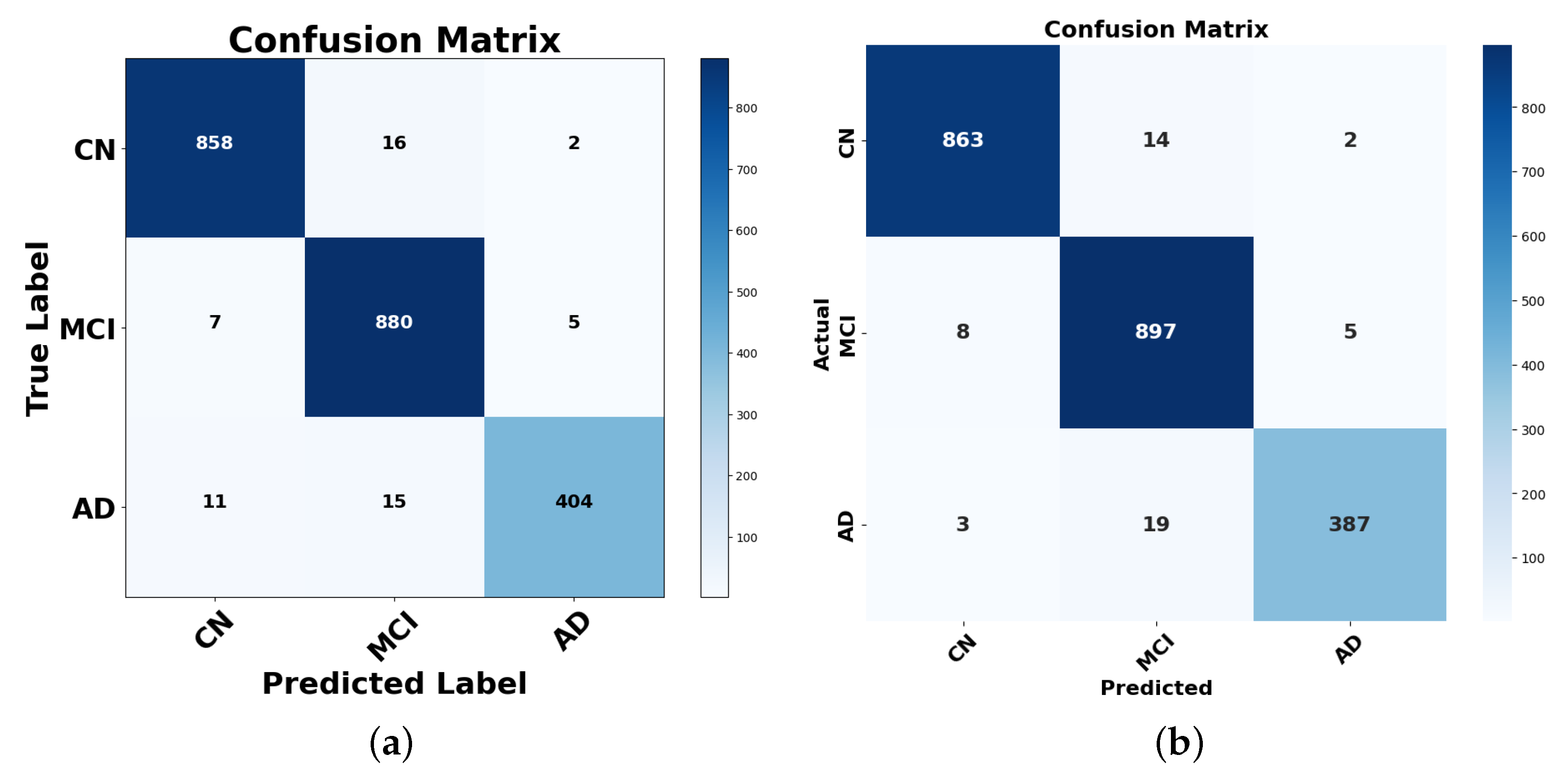
4.1. Performance Analysis Using the Confusion Matrix
4.1.1. Analysis of Misclassifications and Hard Voting Performance
4.1.2. Analysis of Misclassifications and Stacking Performance
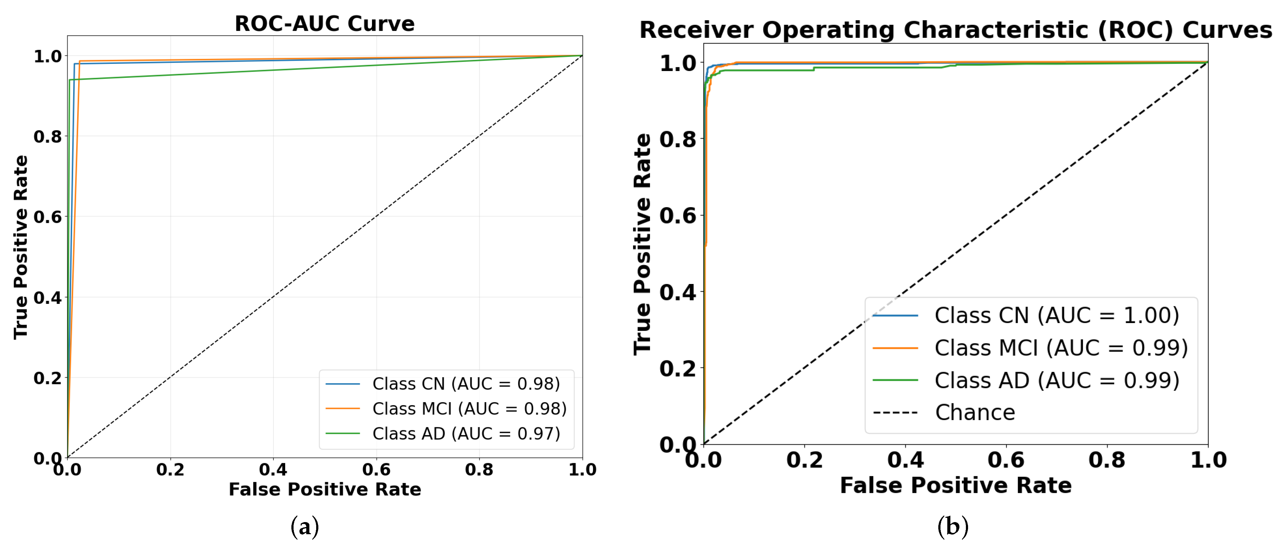
4.2. Performance Evaluation Using ROC and AUC Metrics
- Reasonable progression of difficulty: the slight performance differences between classes (CN being easiest and AD being hardest to classify in hard voting) align with clinical expectations, as cognitive normal cases are typically more distinct than disease states.
- Consistent performance across ensembles: if severe overfitting were present, we might see unrealistically perfect performance across all classes or unexpected patterns (such as AD being easier to classify than CN).
- Ensemble techniques inherently reduce overfitting: the very purpose of ensemble methods is to improve generalization by combining diverse models, which helps mitigate any overfitting present in the individual models.
- Performance ceiling effect: the near-perfect AUC values in the stacking ensemble could represent a genuine ceiling effect rather than overfitting, especially if the classification task is relatively straightforward with well-separated classes.
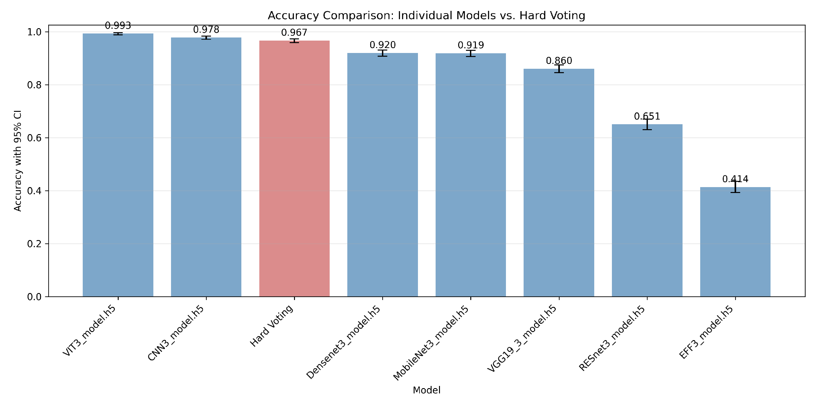
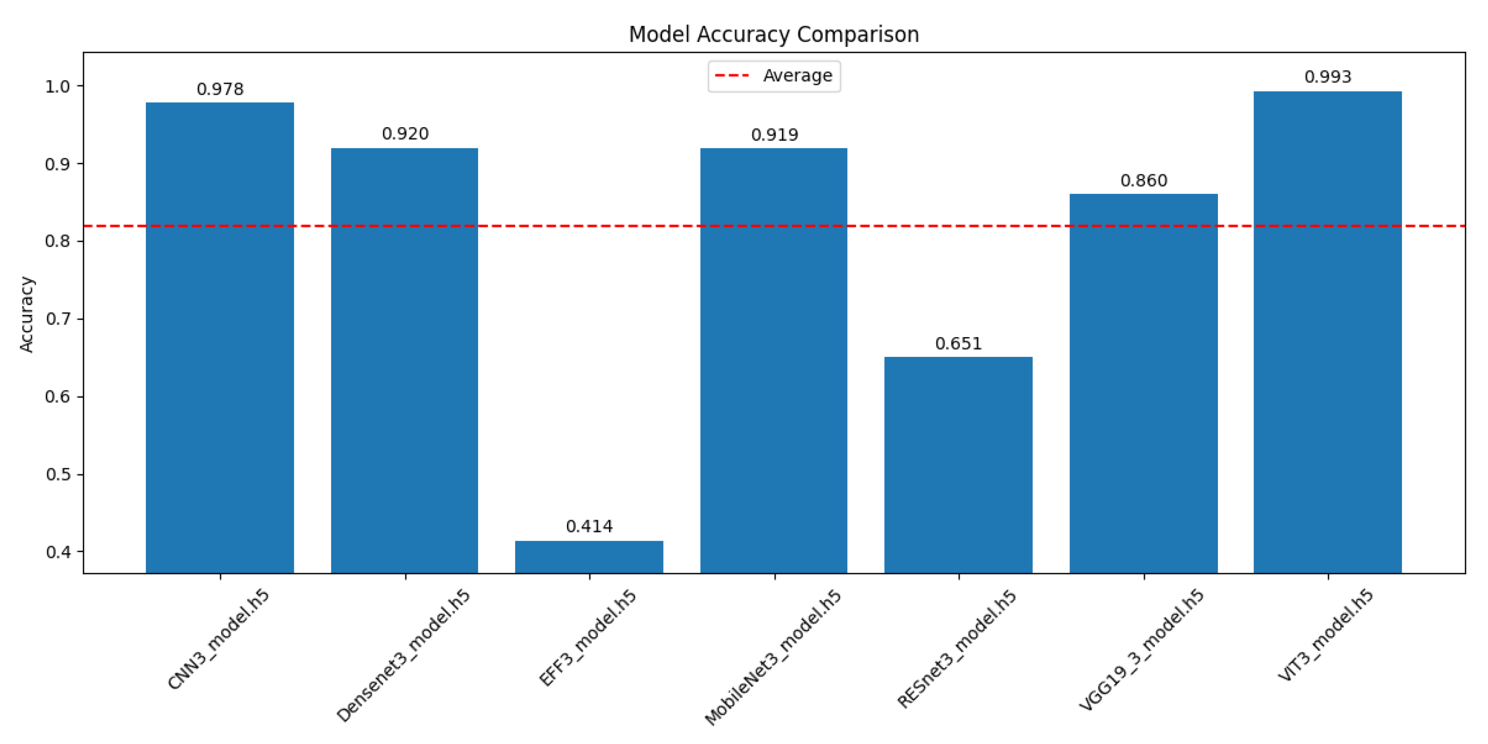
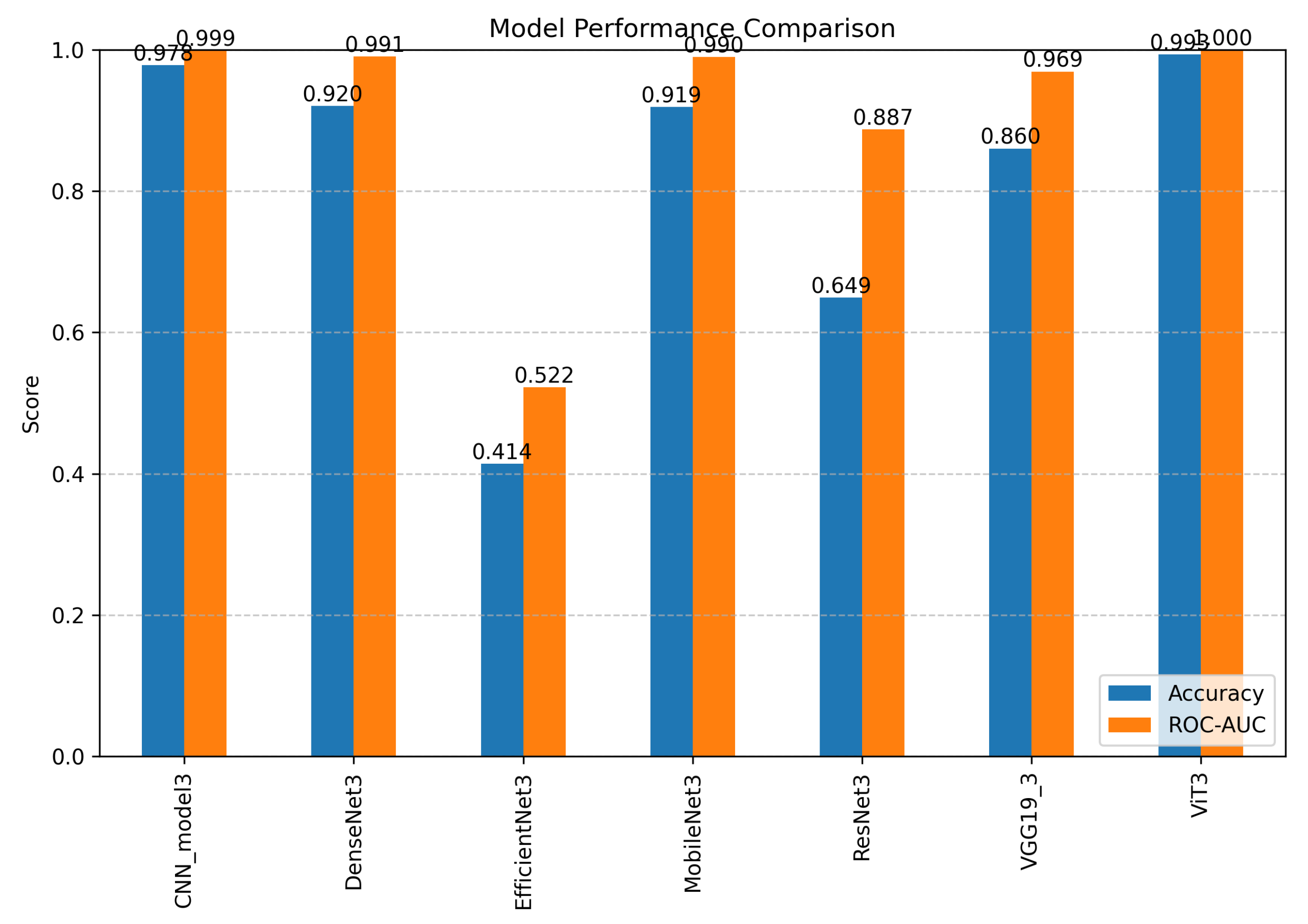
4.3. Comparative Performance Analysis of CNN and Transformer Architectures for Alzheimer’s Disease Progression Detection
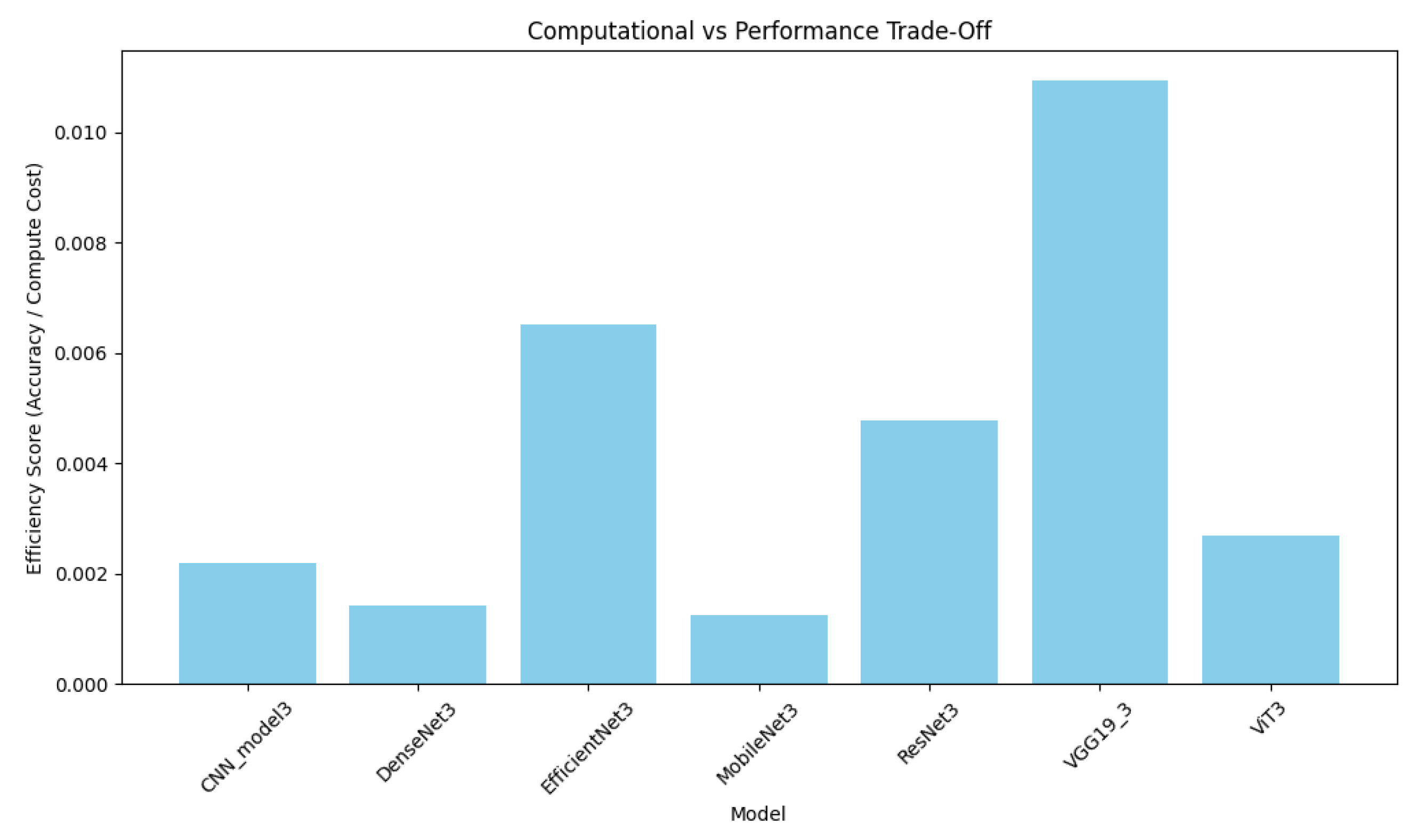
4.4. Computational Efficiency Analysis
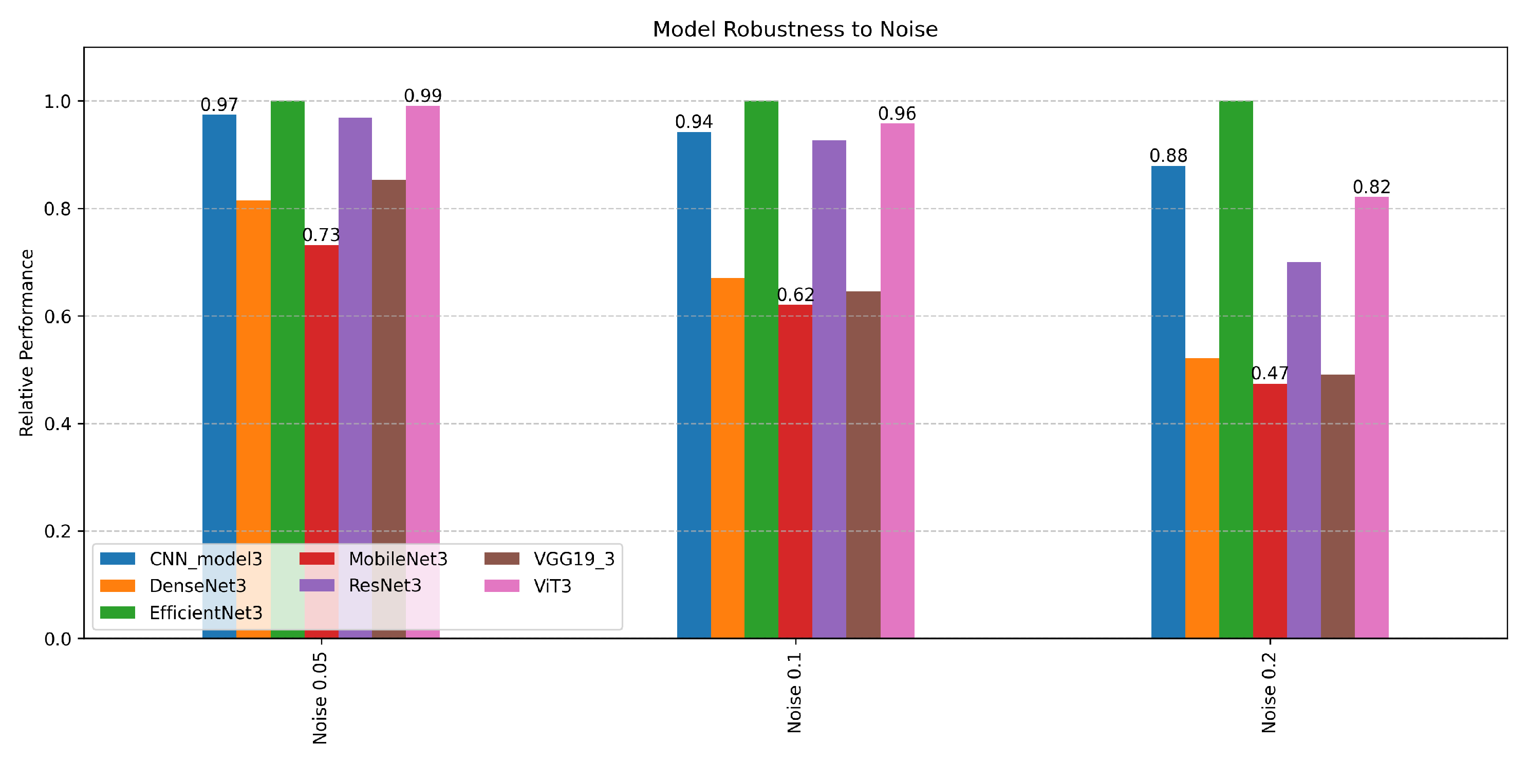
4.4.1. Ensemble Framework Robustness
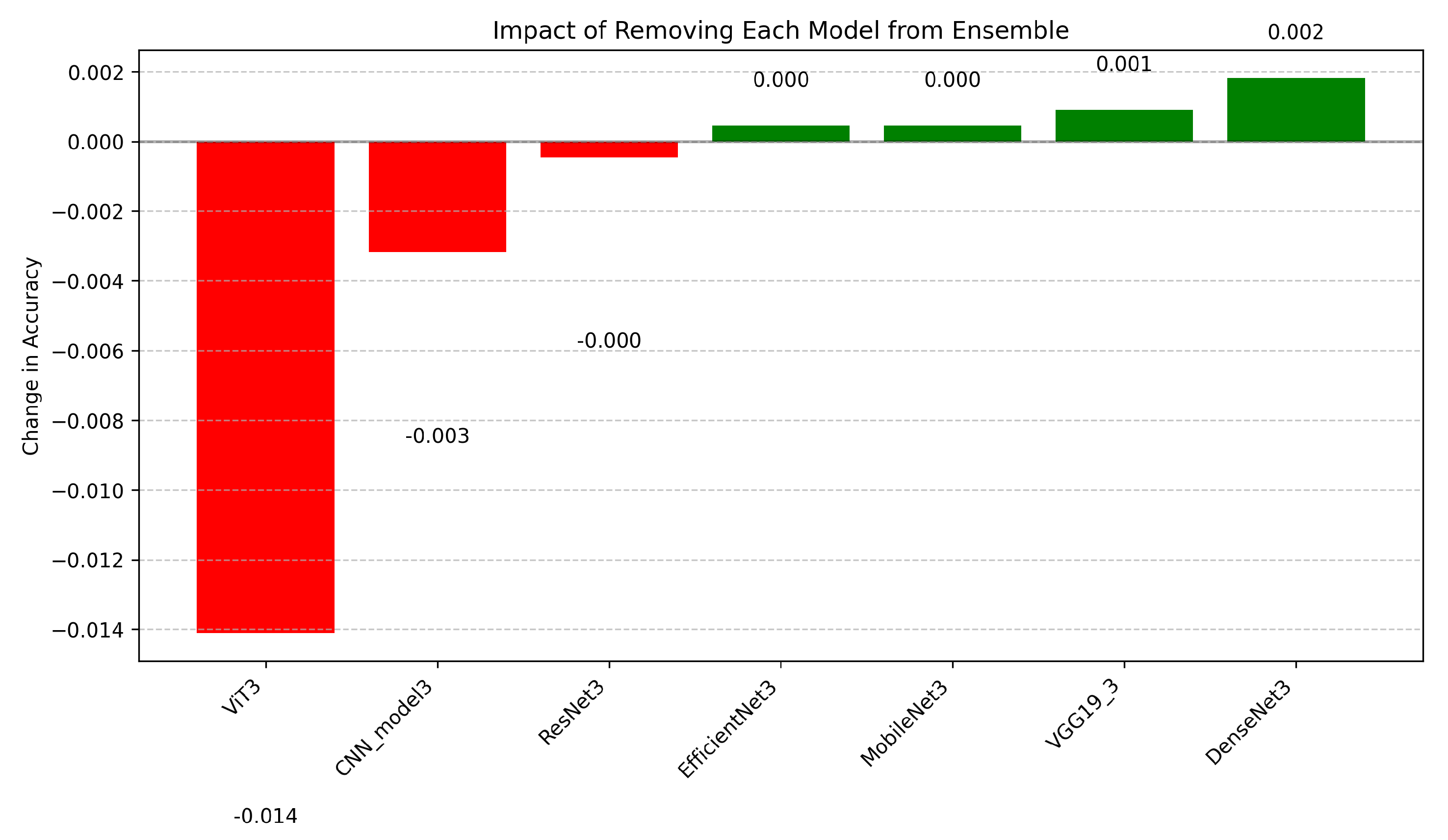
4.4.2. Ablation Study Insights
4.5. Model Trade-Offs
4.6. Comparative Analysis of Ensemble Explainability Techniques
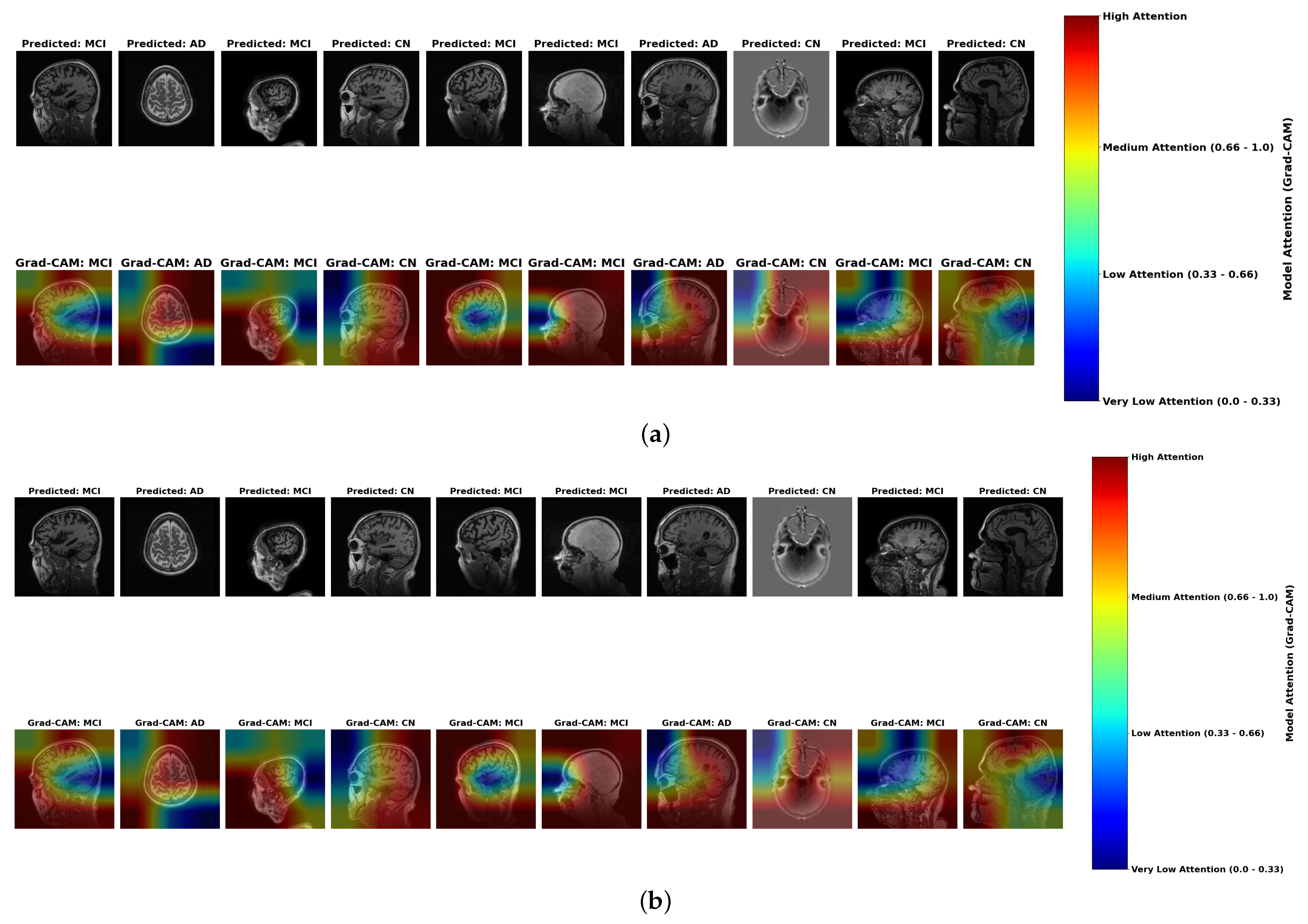
- Color Intensity and Diagnostic Relevance: Grad-CAM visualizations use a color spectrum from blue (very low attention, 0.0–0.33) to red (high attention, 0.66–1.0), revealing where models focus during classification. While both ensemble methods highlight similar regions, subtle but important differences exist in attention distribution. In AD cases, stacking ensembles exhibit slightly more concentrated red regions in medial temporal areas, particularly the hippocampus, indicating more precise focus on established pathological regions. Hard voting shows slightly more diffused yellow-to-red patterns, suggesting less targeted attention. These subtle differences in attention concentration correlate with stacking’s marginally superior accuracy (98.0%) compared to hard voting (97.0%) in Table 2.
- MCI Attention Patterns: For MCI cases, the primary distinction lies in gradient differentiation—stacking displays more nuanced attention gradients with better yellow-to-orange transitions (medium-to-high attention, 0.5–0.8) distributed across temporal-parietal regions, capturing the subtle, widespread changes characteristic of early neurodegeneration. Hard voting shows slightly less intensity differentiation, potentially missing the graduated nature of early pathological changes. These subtle gradient differences may contribute to stacking’s enhanced ability to detect borderline MCI cases, as evidenced by the model performance metrics in Table 8.
- Color Distribution in Misclassifications: Analysis of misclassified cases reveals diagnostic patterns consistent across both ensemble methods. Correctly classified AD cases display concentrated red regions in hippocampal areas, while misclassified cases (particularly AD classified as CN) show inappropriate green-to-blue coloration (low attention, 0.0–0.4) in pathologically significant regions. This color distribution anomaly provides a visual explanation for the classification errors documented in Table 7, where even the best model (ResNet) achieved only 75% accuracy on these critical cases.
4.6.1. LIME Results Comparison
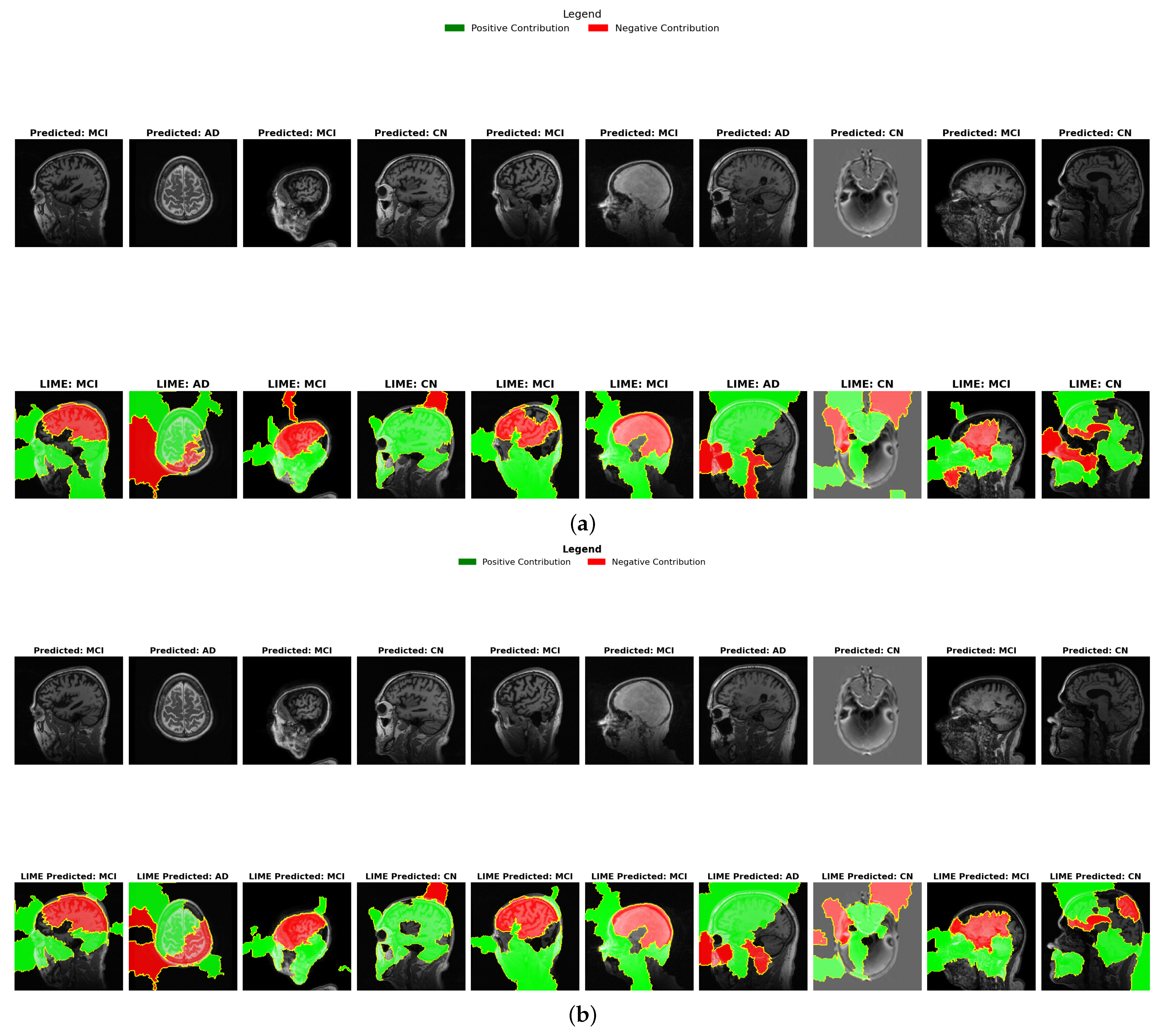
- Binary Feature Attribution (Green vs. Red): Unlike Grad-CAM’s continuous spectrum, LIME provides binary classification of regions as either positively contributing (green) or negatively contributing (red) to the diagnosis. In AD cases, both ensembles show green regions in areas associated with known pathology, but stacking demonstrates more precise positive contribution boundaries, particularly in medial temporal structures. This binary delineation offers clearer interpretability of which specific regions influence diagnostic decisions, supporting stacking’s higher precision (98.0%) reported in Table 2.
- Color Distribution in CN vs. AD: LIME visualizations reveal a diagnostic color inversion between CN and AD cases. CN cases predominantly display red coloration in medial temporal regions, indicating these areas negatively contribute to an AD diagnosis when healthy. Conversely, AD cases show green coloration in these same regions, reflecting positive contribution to diagnosis. This color-based contrastive explanation provides intuitive interpretability that aligns with the clinical understanding of Alzheimer’s progression.
- MCI Contribution Patterns: MCI cases reveal a distinctive mixed pattern of green and red regions. Stacking demonstrates more distributed green areas across cortical regions compared to hard voting, suggesting better sensitivity to the subtle, widespread changes in early neurodegeneration. This distribution difference correlates with the overlap coefficient metrics in Table 9, where higher values indicate better sensitivity to early biomarkers. The balanced color distribution in stacking’s LIME visualizations provides a potential explanation for its superior early detection capabilities.
4.6.2. Saliency Map Results Comparison
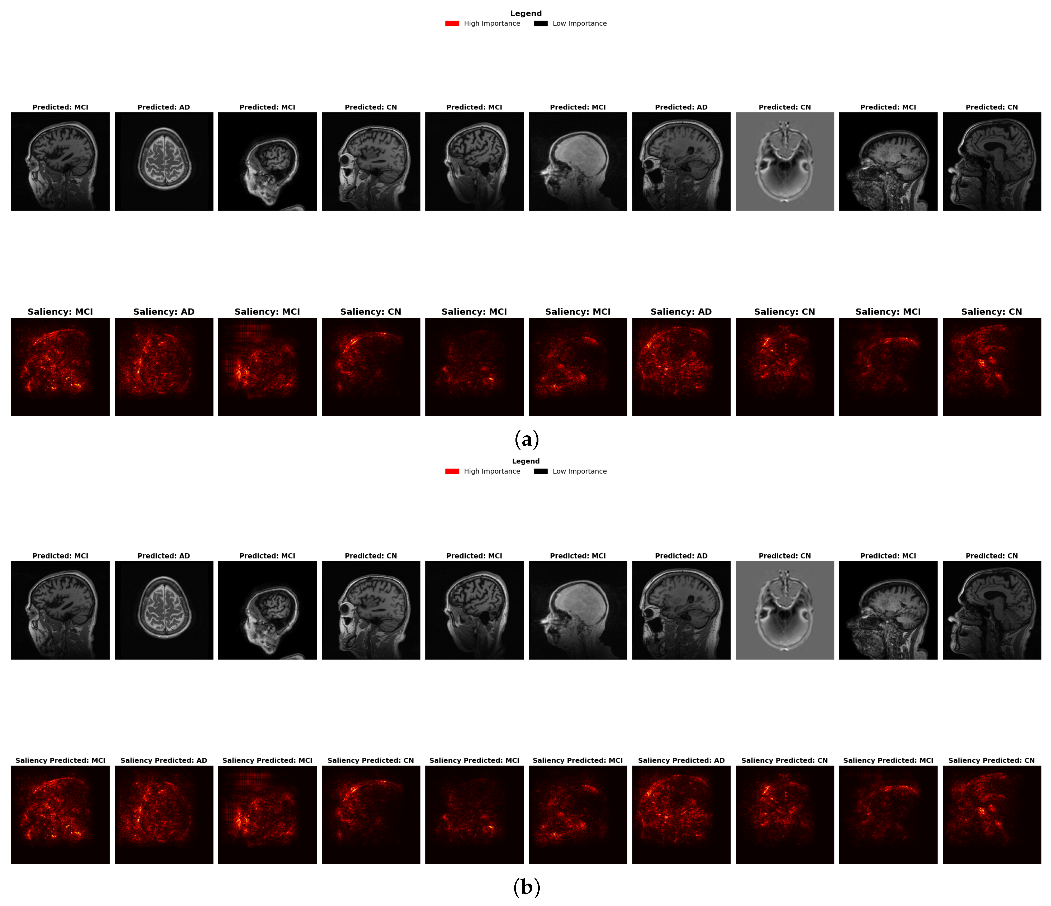
- Brightness Intensity and Diagnostic Focus: Saliency maps visualize feature importance through brightness intensity bright red indicates high importance, while darker areas represent low importance. Both ensembles show similar patterns, though stacking exhibits marginally more concentrated bright spots in the hippocampal and temporal regions, correlating with its slightly superior precision (98.0%).
- Diagnostic-Specific Brightness Patterns: Each diagnostic category shows characteristic brightness distributions across both methods: AD cases with concentrated bright spots in temporal structures, MCI with distributed patterns across broader regions, and CN with fewer, less intense bright spots, validating neuroanatomical progression patterns.
- Early Detection Enhancement: For early-stage MCI, stacking shows slightly more nuanced brightness variations in the cortical and subcortical regions, potentially capturing subtle structural changes indicative of early neurodegeneration, contributing to enhanced sensitivity to early biomarkers (Table 9).
4.7. Comparative Evaluation
5. Conclusions and Future Work
Author Contributions
Funding
Informed Consent Statement
Data Availability Statement
Conflicts of Interest
References
- Razzak, I.; Naz, S.; Ashraf, A.; Khalifa, F.; Bouadjenek, M.R.; Mumtaz, S. Mutliresolutional Ensemble PartialNet for Alzheimer Detection using Magnetic Resonance Imaging Data. Int. J. Intell. Syst. 2022, 37, 3708–3821. [Google Scholar] [CrossRef]
- Alzheimer’s Association Report. 2024 Alzheimer’s disease facts and figures. Alzheimer’S Dement. 2024, 20, 3708–3821. [Google Scholar] [CrossRef] [PubMed]
- Lazarova, S.; Grigorova, D.; Petrova-Antonova, D. Detection of Alzheimer’s Disease Using Logistic Regression and Clock Drawing Errors. Brain Sci. 2023, 13, 1139. [Google Scholar] [CrossRef]
- Golestani, R.; Gharbali, A.; Nazarbaghi, S. Assessment of Linear Discrimination and Nonlinear Discrimination Analysis in Diagnosis Alzheimer’s Disease in Early Stages. Adv. Alzheimer’s Dis. 2020, 9, 21–32. [Google Scholar] [CrossRef]
- Popescu, S.G.; Whittington, A.; Gunn, R.N.; Matthews, P.M.; Glocker, B.; Sharp, D.J.; Cole, J.H.; Initiative, F.T.A.D.N. Nonlinear biomarker interactions in conversion from mild cognitive impairment to Alzheimer’s disease. Hum. Brain Mapp. 2020, 41, 4406–4418. [Google Scholar] [CrossRef] [PubMed]
- Doshi-Velez, F.; Kim, B. Towards a Rigorous Science of Interpretable Machine Learning. arXiv 2017, arXiv:1702.08608. [Google Scholar] [CrossRef]
- Razzak, I.; Naz, S.; Alinejad-Rokny, H.; Nguyen, T.N.; Khalifa, F. A Cascaded Mutliresolution Ensemble Deep Learning Framework for Large Scale Alzheimer’s Disease Detection using Brain MRIs. IEEE/ACM Trans. Comput. Biol. Bioinform. 2024, 21, 573–583. [Google Scholar] [CrossRef]
- Agarwal, S.; Jabbari, S.; Agarwal, C.; Upadhyay, S.; Wu, Z.S.; Lakkaraju, H. Towards the Unification and Robustness of Perturbation and Gradient Based Explanations. In Proceedings of the 38th International Conference on Machine Learning, PMLR 139, Virtual, 18–24 July 2021; Available online: https://arxiv.org/abs/2102.10618 (accessed on 1 March 2024).
- Alami, A.; Boumhidi, J.; Chakir, L. Explainability in CNN-based Deep Learning models for medical image classification. In Proceedings of the International Symposium on Computer Vision, Fez, Morocco, 8–10 May 2024. [Google Scholar] [CrossRef]
- Ribeiro, M.T.; Singh, S.; Guestrin, C. “Why should I trust you?” Explaining the predictions of any classifier. In Proceedings of the ACM SIGKDD International Conference on Knowledge Discovery and Data Mining, New York, NY, USA, 13–17 August 2016; pp. 1135–1144. [Google Scholar] [CrossRef]
- Rezk, N.G.; Alshathri, S.; Sayed, A.; Hemdan, E.E.-D.; El-Behery, H. XAI-Augmented Voting Ensemble Models for Heart Disease Prediction: A SHAP and LIME-Based Approach. Bioengineering 2024, 11, 1016. [Google Scholar] [CrossRef]
- Bloch, L.; Friedrich, C.M. Systematic comparison of 3D Deep learning and classical machine learning explanations for Alzheimer’s Disease detection. Comput. Biol. Med. 2024, 170, 108029. [Google Scholar] [CrossRef]
- Sattarzadeh, S.; Sudhakar, M.; Plataniotis, K.N.; Jang, J.; Jeong, Y.; Kim, H. Integrated Grad-Cam: Sensitivity-Aware Visual Explanation of Deep Convolutional Networks Via Integrated Gradient-Based Scoring. In Proceedings of the ICASSP 2021—2021 IEEE International Conference on Acoustics, Speech and Signal Processing (ICASSP), Toronto, ON, Canada, 6–11 June 2021; pp. 1775–1779. [Google Scholar] [CrossRef]
- Shah, S.T.H.; Khan, I.I.; Imran, A.; Shah, S.B.H.; Mehmood, A.; Qureshi, S.A.; Raza, M.; Di Terlizzi, A.; Cavagliá, M.; Deriu, M.A. Data-driven classification and explainable-AI in the field of lung imaging. Front. Big Data 2024, 7, 1393758. [Google Scholar] [CrossRef]
- Salahuddin, Z.; Woodruff, H.C.; Chatterjee, A.; Lambin, P. Transparency of Deep Neural Networks for Medical Image Analysis: A Review of Interpretability Methods. Comput. Biol. Med. 2022, 140, 105111. Available online: https://arxiv.org/abs/2212.10565 (accessed on 1 March 2024). [CrossRef]
- Ijiga, A.C.; Igbede, M.A.; Ukaegbu, C.; Olatunde, T.I.; Olajide, F.I.; Enyejo, L.A. Precision healthcare analytics: Integrating ML for automated image interpretation, disease detection, and prognosis prediction. World J. Biol. Pharm. Health Sci. 2024, 18, 336–354. [Google Scholar] [CrossRef]
- Shivhare, I.; Jogani, V.; Purohit, J.; Shrawne, S.C. Analysis of Explainable Artificial Intelligence Methods on Medical Image Classification. In Proceedings of the International Conference on Artificial Intelligence and Emerging Technologies, Bhilai, India, 5–6 January 2023. [Google Scholar] [CrossRef]
- Rodrigues, C.M.; Boutry, N.; Najman, L. Transforming gradient-based techniques into interpretable methods. Pattern Recognit. Lett. 2024, 184, 66–73. [Google Scholar] [CrossRef]
- Muzellec, S.; Andéol, L.; Fel, T.; VanRullen, R.; Serre, T. Gradient strikes back: How filtering out high frequencies improves explanations. arXiv 2023, arXiv:2307.09591. [Google Scholar]
- Pelka, O.; Friedrich, C.M.; Nensa, F.; Mönninghoff, C.; Bloch, L.; Jöckel, K.-H.; Schramm, S.; Hoffmann, S.S.; Winkler, A.; Weimar, C.; et al. Sociodemographic data and APOE-ε4 augmentation for MRI-based detection of amnestic mild cognitive impairment using deep learning systems. PLoS ONE 2020, 15, e0236868. [Google Scholar] [CrossRef] [PubMed]
- Zeineldin, R.A.; Karar, M.E.; Elshaer, Z.; Coburger, J.; Wirtz, C.R.; Burgert, O.; Mathis-Ullrich, F. Explainability of deep neural networks for MRI analysis of brain tumors. Int. J. Comput. Assist. Radiol. Surg. 2022, 17, 1673–1683. [Google Scholar] [CrossRef] [PubMed]
- Rahman, M.M.; Lewis, N.; Plis, S. Geometrically Guided Integrated Gradients. arXiv 2022, arXiv:2206.05903. [Google Scholar]
- Band, S.S.; Yarahmadi, A.; Hsu, C.-C.; Biyari, M.; Sookhak, M.; Ameri, R.; Dehzangi, I.; Chronopoulos, A.T.; Liang, H.-W. Application of explainable Artificial Intelligence in Medical Health: A Systematic Review of Interpretability Methods. Inf. Med. Unlock. 2023, 40, 101286. [Google Scholar] [CrossRef]
- Qiu, L.; Yang, Y.; Cao, C.C.; Zheng, Y.; Ngai, H.; Hsiao, J.; Chen, L. Generating Perturbation-based Explanations with Robustness to Out-of-Distribution Data. In Proceedings of the ACM Web Conference 2022, New York, NY, USA, 25–29 April 2022. [Google Scholar] [CrossRef]
- Alzheimer’s Disease Neuroimaging Initiative. ADNI Data and Samples. 2024. Available online: https://adni.loni.usc.edu/data-samples/adni-data/ (accessed on 1 January 2025).
- Wolpert, D.H. Stacked generalization. Neural Netw. 1992, 5, 241–259. [Google Scholar] [CrossRef]
- Bonab, H.; Can, F. Less Is More: A Comprehensive Framework for the Number of Components of Ensemble Classifiers. arXiv 2017, arXiv:1709.02925. [Google Scholar] [CrossRef]
- Pedregosa, F.; Varoquaux, G.; Gramfort, A.; Michel, V.; Thirion, B.; Grisel, O.; Blondel, M.; Prettenhofer, P.; Weiss, R.; Dubourg, V.; et al. Scikit-learn: Machine Learning in Python. J. Mach. Learn. Res. 2011, 12, 2825–2830. [Google Scholar]
- He, H.; Garcia, E.A. Learning from Imbalanced Data. IEEE Trans. Knowl. Data Eng. 2009, 21, 1263–1284. [Google Scholar] [CrossRef]
- Richardson, E.; Trevizani, R.; Greenbaum, J.A.; Carter, H.; Nielsen, M.; Peters, B. The Receiver Operating Characteristic Curve Accurately Assesses Imbalanced Datasets. Patterns 2024, 5, 100994. [Google Scholar] [CrossRef]
- Adarsh, V.; Gangadharan, G.R.; Fiore, U.; Zanetti, P. Multimodal classification of Alzheimer’s disease and Mild Cognitive Impairment using Custom MKSCDDL Kernel over CNN with Transparent Decision-Making for Explainable Diagnosis. Sci. Rep. 2024, 14, 1774. [Google Scholar] [CrossRef]
- Mahmud, T.; Barua, K.; Habiba, S.U.; Sharmen, N.; Hossain, M.S.; Andersson, K. An Explainable AI Paradigm for Alzheimer’s Diagnosis Using Deep Transfer Learning. Diagnostics 2024, 14, 345. [Google Scholar] [CrossRef]
- Duamwan, L.M.; Bird, J.J. Explainable AI for Medical Image Processing: A Study on MRI in Alzheimer’s Disease. In Proceedings of the PETRA ’23: Proceedings of the 16th International Conference on Pervasive Technologies Related to Assistive Environments, Corfu, Greece, 5–7 July 2023; pp. 480–484. [Google Scholar] [CrossRef]
- El-Sappagh, S.; Alonso, J.M.; Islam, S.M.R.; Sultan, A.M.; Kwak, K.S. A multilayer multimodal detection and prediction model based on explainable artificial intelligence for Alzheimer’s disease. Sci. Rep. 2021, 11, 2660. [Google Scholar] [CrossRef] [PubMed]


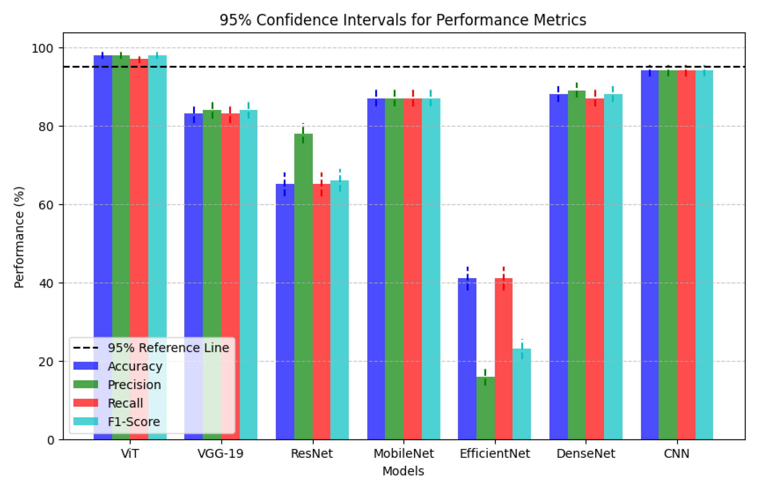
| Models | Accuracy | Precision | Recall | F1-Score |
|---|---|---|---|---|
| ViT | 98.0% | 98.0% | 97.0% | 98.0% |
| VGG-19 | 83.0% | 84.0% | 83.0% | 84.0% |
| ResNet | 65.0% | 78.0% | 65.0% | 66.0% |
| MobileNet | 87.0% | 87.0% | 87.0% | 87.0% |
| EfficientNet | 41.0% | 16.0% | 41.0% | 23.0% |
| DenseNet | 88.0% | 89.0% | 87.0% | 88.0% |
| CNN | 94.0% | 94.0% | 94.0% | 94.0% |
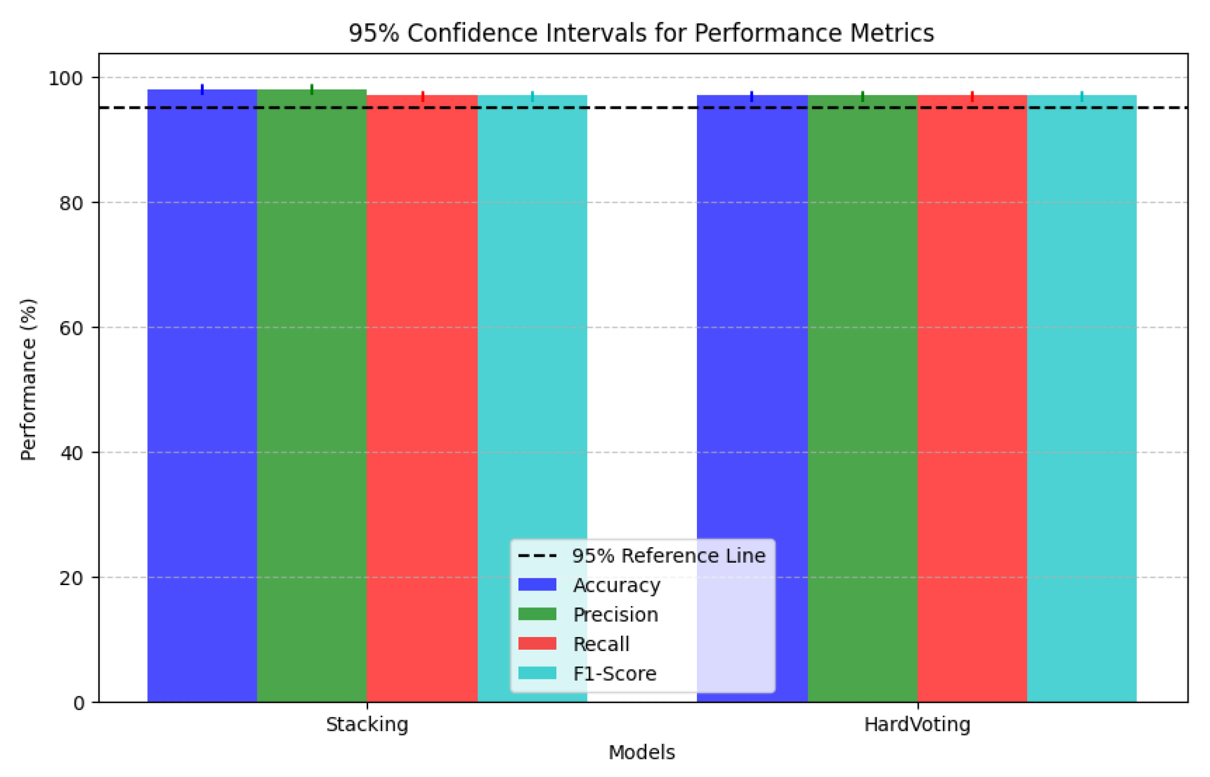
| Ensemble Techniques | Accuracy | Precision | Recall | F1-Score |
|---|---|---|---|---|
| Stacking | 98.0% | 98.0% | 97.0% | 97.0% |
| Hard Voting | 97.0% | 97.0% | 97.0% | 97.0% |
| Model | CN→MCI (FP) | MCI→AD (FP) | MCI→CN (FN) | AD→MCI (FN) |
|---|---|---|---|---|
| ViT3 | 0.17% | 0.65% | 0.17% | 0.65% |
| CNN_model3 | 1.52% | 1.59% | 1.52% | 1.59% |
| DenseNet3 | 5.25% | 4.69% | 5.25% | 4.69% |
| MobileNet3 | 5.62% | 4.18% | 5.62% | 4.18% |
| VGG19_3 | 7.84% | 8.08% | 7.84% | 8.08% |
| ResNet3 | 6.92% | 22.70% | 6.92% | 22.70% |
| EfficientNet3 | 50.00% | 50.00% | 50.00% | 50.00% |
| Error Type | % of Errors | Error Category | Clinical Impact | Best Models | Best Accuracy | VIT Accuracy |
|---|---|---|---|---|---|---|
| 2→0 | 44.44% | False Negative | High | ResNet | 75.00% | 0.00% |
| 0→1 | 22.22% | False Positive | Medium | DenseNet, VGG19 | 100.00% | 0.00% |
| 1→2 | 11.11% | False Positive | Medium–High | Multiple | 100.00% | 0.00% |
| 2→1 | 11.11% | False Negative | High | DenseNet | 100.00% | 0.00% |
| 1→0 | 11.11% | False Negative | Medium–High | Multiple | 100.00% | 0.00% |
| Model | 2→0 (4) | 0→1 (2) | 1→2 (1) | 2→1 (1) | 1→0 (1) | Overall |
|---|---|---|---|---|---|---|
| DenseNet | 0.00% | 100.00% | 100.00% | 100.00% | 0.00% | 44.44% |
| ResNet | 75.00% | 50.00% | 0.00% | 0.00% | 0.00% | 44.44% |
| VGG19 | 25.00% | 100.00% | 0.00% | 0.00% | 100.00% | 44.44% |
| CNN | 25.00% | 50.00% | 0.00% | 0.00% | 100.00% | 33.33% |
| EfficientNet | 0.00% | 0.00% | 100.00% | 0.00% | 100.00% | 22.22% |
| MobileNet | 0.00% | 50.00% | 100.00% | 0.00% | 0.00% | 22.22% |
| ViT | 0.00% | 0.00% | 0.00% | 0.00% | 0.00% | 0.00% |
| Error Type | Instance Index | Correct Models | # Correct | % Agreement |
|---|---|---|---|---|
| 2→0 | 604 | CNN, ResNet | 2/7 | 28.57% |
| 2→0 | 1224 | ResNet | 1/7 | 14.29% |
| 2→0 | 2045 | VGG19 | 1/7 | 14.29% |
| 2→0 | 2116 | ResNet | 1/7 | 14.29% |
| 0→1 | 1353 | CNN, DenseNet, VGG19 | 3/7 | 42.86% |
| 0→1 | 1550 | Multiple | 4/7 | 57.14% |
| 1→2 | 487 | Multiple | 3/7 | 42.86% |
| 2→1 | 1326 | DenseNet | 1/7 | 14.29% |
| 1→0 | 1798 | Multiple | 3/7 | 42.86% |
| Model | Correct 2→0 | % Correct | False Negative Rate |
|---|---|---|---|
| ResNet | 3/4 | 75.00% | 25.00% |
| CNN | 1/4 | 25.00% | 75.00% |
| VGG19 | 1/4 | 25.00% | 75.00% |
| DenseNet | 0/4 | 0.00% | 100.00% |
| EfficientNet | 0/4 | 0.00% | 100.00% |
| MobileNet | 0/4 | 0.00% | 100.00% |
| ViT | 0/4 | 0.00% | 100.00% |
| Architecture | MCI Accuracy | Misclassified as CN | Misclassified as AD | Mean Confidence | Mean Uncertainty |
|---|---|---|---|---|---|
| ViT | 99.78% | 0.11% | 0.11% | 0.998 | 0.004 |
| EfficientNet | 100.00% | 0.00% | 0.00% | 0.399 | 1.533 |
| CNN | 98.46% | 1.43% | 0.11% | 0.979 | 0.054 |
| DenseNet | 94.07% | 4.84% | 1.10% | 0.890 | 0.350 |
| MobileNet | 93.19% | 6.26% | 0.55% | 0.877 | 0.369 |
| VGG19 | 89.78% | 5.16% | 5.05% | 0.806 | 0.561 |
| ResNet | 50.66% | 7.25% | 42.09% | 0.522 | 0.713 |
| Architecture | Overlap Coefficient | Confusion Rate | Confidence Gap |
|---|---|---|---|
| EfficientNet | 0.9500 | 0.5000 | 0.0000 |
| ViT | 0.9423 | 0.0017 | 0.0017 |
| CNN | 0.9270 | 0.0152 | 0.0032 |
| MobileNet | 0.8980 | 0.0562 | 0.0062 |
| DenseNet | 0.8956 | 0.0525 | 0.0122 |
| VGG19 | 0.8668 | 0.0784 | 0.0097 |
| ResNet | 0.8055 | 0.0692 | 0.0143 |
| Architecture | Confidence Mean | Confidence Std | Mean Entropy | Max Entropy | Difficult Cases |
|---|---|---|---|---|---|
| ViT | 0.998 | 0.035 | 0.004 | 1.024 | 91 |
| CNN | 0.979 | 0.108 | 0.054 | 1.545 | 91 |
| DenseNet | 0.890 | 0.191 | 0.350 | 1.582 | 91 |
| MobileNet | 0.877 | 0.211 | 0.369 | 1.578 | 91 |
| VGG19 | 0.806 | 0.241 | 0.561 | 1.580 | 91 |
| ResNet | 0.522 | 0.365 | 0.713 | 1.585 | 91 |
| EfficientNet | 0.399 | 0.001 | 1.533 | 1.538 | 91 |
| Architecture | Overlap Coefficient | Confusion Rate | Confidence Gap |
|---|---|---|---|
| ViT | 0.9286 | 0.0065 | 0.0038 |
| CNN | 0.8958 | 0.0159 | 0.0087 |
| VGG19 | 0.8222 | 0.0808 | 0.0616 |
| DenseNet | 0.8191 | 0.0469 | 0.0128 |
| MobileNet | 0.8323 | 0.0418 | 0.0281 |
| ResNet | 0.5673 | 0.2270 | 0.0312 |
| EfficientNet | 0.0000 | 0.5000 | 0.0000 |
| Architecture | Interpretability Score | Visualization Approach | Biomarker Alignment | Clinical Explainability | Region Specificity |
|---|---|---|---|---|---|
| CNN | High | Gradient-based | High | High | High |
| ResNet | High | Gradient-based | High | High | High |
| VGG19 | High | Gradient-based | High | High | Medium |
| DenseNet | High | Gradient-based | High | High | Medium |
| EfficientNet | Medium–High | Efficient feature | High | Medium | Medium |
| MobileNet | Medium–High | Efficient feature | High | Medium | Medium |
| ViT | Medium | Attention-based | Medium | Medium | Medium |
| Model | Size (MB) | Parameters (M) | Layers | Avg. Inference Time (ms) | Memory Usage (MB) | Trainable/Non-Trainable |
|---|---|---|---|---|---|---|
| CNN | 27.62 | 7.24 | 20 | 0.43 | 1027.84 | 7.24 M/0 |
| DenseNet | 79.93 | 20.95 | 718 | 2.92 | 222.47 | 2.63 M/18.33 M |
| EfficientNet | 22.99 | 6.03 | 249 | 1.55 | 40.95 | 3.32 M/2.70 M |
| MobileNet | 16.12 | 4.23 | 162 | 0.97 | 766.00 | 1.97 M/2.26 M |
| ResNet | 100.49 | 26.34 | 183 | 1.64 | 83.51 | 11.69 M/14.66 M |
| VGG19 | 127.04 | 33.30 | 39 | 2.18 | 36.14 | 13.26 M/20.04 M |
| ViT | 332.34 | 87.12 | 27 | 5.15 | 71.95 | 87.12 M/0.003 M |
| Ref | Classifier | Best Accuracy Score | XAI Method | Dataset |
|---|---|---|---|---|
| Mahmud et al. [32] | DenseNet169 and DenseNet201 | 96.00% | Saliency Maps, Grad-CAM | MRI Scans OASIS |
| Duamwan et al. [33] | CNN | 94.96% | LIME | ADNI MRI |
| El-Sappag et al. [34] | Random Forest | 93.95% | SHAP | ADNI Multimodal with 12 Features |
| Adarsh et al. [31] | CNN + MKSCDDL + Scandent Decision Trees | 98.27% | Scandent Decision Trees, Discriminative Dictionary Learning | ADNI MRI |
| This Study | Stacking Ensemble | 98.00% | Grad-CAM, LIME, Saliency Map | ADNI MRI |
Disclaimer/Publisher’s Note: The statements, opinions and data contained in all publications are solely those of the individual author(s) and contributor(s) and not of MDPI and/or the editor(s). MDPI and/or the editor(s) disclaim responsibility for any injury to people or property resulting from any ideas, methods, instructions or products referred to in the content. |
© 2025 by the authors. Licensee MDPI, Basel, Switzerland. This article is an open access article distributed under the terms and conditions of the Creative Commons Attribution (CC BY) license (https://creativecommons.org/licenses/by/4.0/).
Share and Cite
Adeniran, O.T.; Ojeme, B.; Ajibola, T.E.; Peter, O.O.E.; Ajala, A.O.; Rahman, M.M.; Khalifa, F. Explainable MRI-Based Ensemble Learnable Architecture for Alzheimer’s Disease Detection. Algorithms 2025, 18, 163. https://doi.org/10.3390/a18030163
Adeniran OT, Ojeme B, Ajibola TE, Peter OOE, Ajala AO, Rahman MM, Khalifa F. Explainable MRI-Based Ensemble Learnable Architecture for Alzheimer’s Disease Detection. Algorithms. 2025; 18(3):163. https://doi.org/10.3390/a18030163
Chicago/Turabian StyleAdeniran, Opeyemi Taiwo, Blessing Ojeme, Temitope Ezekiel Ajibola, Ojonugwa Oluwafemi Ejiga Peter, Abiola Olayinka Ajala, Md Mahmudur Rahman, and Fahmi Khalifa. 2025. "Explainable MRI-Based Ensemble Learnable Architecture for Alzheimer’s Disease Detection" Algorithms 18, no. 3: 163. https://doi.org/10.3390/a18030163
APA StyleAdeniran, O. T., Ojeme, B., Ajibola, T. E., Peter, O. O. E., Ajala, A. O., Rahman, M. M., & Khalifa, F. (2025). Explainable MRI-Based Ensemble Learnable Architecture for Alzheimer’s Disease Detection. Algorithms, 18(3), 163. https://doi.org/10.3390/a18030163