Control of High-Power Slip Ring Induction Generator Wind Turbines at Variable Wind Speeds in Optimal and Reliable Modes

Abstract

This work analyzes high-power wind turbines (WTs) from the Oravita region, Romania. These WTs are based on slip ring induction generator with wound rotor and we propose a modified architecture with two power converters on both the stator and on the rotor, functioning at variable wind speeds spanning a large interval. Investigations developed around a realistic WT model with doubly fed induction generator show how WT control enables variable wind speed operations at optimal mechanical angular speed (MAS), guaranteeing maximal power point (MPP), but only up to a critical wind speed value, after which the electrical power must saturate for reliable operation. In this reliable operating region, blade pitch angle control must be enforced. Variable wind speed acts as a time-varying parameter disturbance but also imposes the MPP operation setpoint in one of the two analyzed regions. To achieve null tracking errors, a double integrator must appear within the MAS controller when the wind speed disturbance is realistically modeled as a ramp-like input; however, inspecting the linearized model reveals several difficulties as described in the paper, together with the proposed solution tradeoff. The study developed around the Fuhrlander-FL-MD-70 1.5[MW] WT model shows that several competitive controllers are designed and tested in the identified operating regions of interest, as they validate the reliable and performant functioning specifications.

1. Introduction

This work analyzes functioning regimes for high-power wind turbines (WTs) with wound rotor induction generators, at large wind speed variations under the requirement of optimal operation at maximum power point (MPP). The wind speed value $V\left(t\right)$ is fundamental in this context, as it imposes the optimal mechanical angular speed (MAS), $n_{OPTIM}$, that ensures MPP operation for the WT.

To this day, WTs have developed a variety of types and sizes, some reaching up to 6 [MW] installed capacity and with blades diameters up to 150 [m]. Repurposed for either small area operations (even for personal locations used within islanded micro-grids) or for mass energy production in wind farms covering large areas (sometimes offshore), the WTs capture and convert the wind energy to electric energy that is meant to be delivered to some electrical grid to which the WTs are connected. To this end, the main research topics revolve around modeling [1,2,3,4,5], control [6,7,8,9] and operation analysis [10,11,12,13].

On the power transformation pipeline, a series of energy transformations occur which must be optimized from an efficiency point of view by the designers/manufacturers [10,11,12,13,14,15]. In this respect, there are WTs with or without a reducer. In reducer-based ones with ratios beyond 1:100 with the generator having nominal MAS of about 3000 [rpm], power losses occur; however, the generator mass is small [16,17,18,19,20]. In those without a reducer mechanism, there are no additional power losses, but the generator mass must be carefully designed in order to work at such small MAS, while the materials needed for producing such a device have significantly higher costs (supermagnet alloys from neodymium, iron, boron—Nd2Fe14B) [21,22,23].

Modern WTs are equipped with blade pitch angle control systems; therefore, when the wind speeds are too high, the angle of attack of the blade is adapted to keep the MAS within safe bounds. The blade angle typically varies from 0 to 90 angular degrees, with the higher-end value being applied to stop the WT’s rotor during violent windstorms. A blade pitch angle control system bases its feedback on anemometer measurements for wind speed and on the MAS (or the generated electrical power).

Remark 1. 

Automatic blade pitch angle control also keeps the energy conversion in reliable condition by avoiding mechanical stress in the WT’s tower structure, within bearing and within the transmission elements. Hence, it increases the WT lifespan and decreases the maintenance costs. It is due to this that the blades pitch angle $\beta$ is based on three independent actuation systems powered by alternative energy sources.

In the specialized literature, only induction generators with wound rotors having a single power converter in the rotor are generally analyzed (see works [10,11,12,13,17,18,19,20]). In this work, we analyze the induction generator with two power converters in both the stator and in the rotor. In the Oravita (Romania) region, there are six Fuhrlander FL-MD-70 WTs of 1.5 [MW] capacity, each equipped with an induction generator with a wound rotor [24]. In this case, by imposing the rotor voltage $U_R$, the optimal MAS can be tracked. The value $U_R$ is intended to control the additional rotor resistance $R_{ad}$. The group of six WTs from Oravita work at wind speeds ranging from 3 up to 25 [m/s], then the MAS, depending linearly on the wind speed, should adapt within its own range at a ratio of about 3/25 = 1/8.3333 set by the wind speed variation. At this high wind speed variation, two power converters are needed: one in the stator circuit controllable by the stator frequency $f$, which delivers the stator power $P_{stator}$, and a second converter for the rotor, which is responsible for the rotor delivered power $P_{rotor}$ [25,26,27].

Remark 2. 

The power converter from the rotor circuit changes the rotor resistance through the rotor voltage in a way that, apparently, an additional $R_{ad}$ resistance is introduced.

The wind speed variation is divided into two regions. The first one ranges within [3; 11] [m/s] and corresponds to small to medium wind speeds. The second one is [11; 25] [m/s] and corresponds to high wind speeds. In the first interval, the WT operates in MPP, with optimal MAS at the value $n_{OPTIM}$, with optimal stator frequency value $f_{OPTIM}$ and with optimal rotor additional resistance $R_{ad-OPTIM}$. These values are realized by the stator power converter for $f_{OPTIM}$ and by the rotor power converter for $R_{ad-OPTIM}$. In the second range, for limiting the electrical and mechanical stress within admissible bounds, under high wind speeds, both the WT power and MAS are saturated; the WT power is regulated through the blade pitch angle $\beta$, while the generator power is characterized by the stator working at constant frequency $f$ and the rotor working at constant $R_{ad}$ actuated by the rotor converter. In this regime, the generator power changes only subject to the MAS value $n$ but it is the WT power characteristic selected as the controller quantity.

Remark 3. 

In the first interval corresponding to small up to medium wind speeds, the blade pitch angle β = 0 is constant, while in the second interval, it is changed as it enters the active control role.

Recent results on blade pitch angle control are analyzed from the literature. Improved WT operation under individual pitch control was proposed by the authors of [28]. A linear quadratic pitch angle controller was designed for a variable speed WT of 850 [kW] in [29]. Intelligent genetic algorithms were used to optimize the parameters of a PID for WT blade pitch controller in [30], while for WT load mitigation, individual pitch controllers were proposed by Han et al. in [31]. Comparisons of different metaheuristic optimizers were provided by the authors of [32] for the same blade pitch control problem. A similar optimal-based control approach is followed by [33] but for a doubly fed induction generator in WT, based on evolutionary algorithm. Machine learning is a novel approach dedicated to pitch angle control in WTs and was among the first reported in the work of [34,35]. Actuator faults were considered for improving the load mitigation in WTs through fault-tolerant pitch control by the authors of [36]. Yet another machine learning control, this time a reinforcement learning approach, was proposed for the same control problem in the work [37]. A wider and theoretically oriented work towards stability analysis under several controllers is proposed in [38]. Under large wind speed variation, which is also the topic of concern in this work, the pitch control was considered by Chen et al. in [39]. Adaptive control for improved tracking performance of WTs through blade pitch angle control is proposed by Zhou et al. in [40]. For offshore WTs, the control robustness issue under high wind and waves was considered and proven feasible by the authors of the work [41].

For variable speed wind turbine operation, the wind speed is the most important factor, as it is simultaneously a time-varying parameter in the dynamical model and also imposes the optimal MAS reference input value to ensure MPP tracking. On short time intervals lasting from several seconds to several tens of seconds, the wind speed can be accepted to follow a ramp-like temporal variation schedule. In effect, this also drives a ramp-like MAS reference input variation. The internal model principle in control requires a double integrator to ensure null steady state tracking error; however, the WT model analyzed in this work shows that this is not possible in the operating region where MAS control is required, so a tradeoff must be made. On the other hand, at higher wind speeds, corresponding to the operating region where the blade pitch angle is used to control the WT power, the linearized dynamics show that a double integrator is feasible and therefore implemented.

Different from the analyzed literature, this paper works out several distinct contributions. First, a real-world case study analysis is proposed, based on WT models operating in the Oravita region, Romania. Secondly, the high wind speed variation in continental locations forces the WTs to operate in different regions, aimed at either maximum operation efficiency (maximum power point) or at maximally reliable operation through saturation of the powers and MAS. This aspect is clearly analyzed in our work. Thirdly, with two identified operating regions corresponding to small wind speeds and large wind speeds, feasible control is proposed dedicated to improved tracking performance under disturbance rejection. For this, realistic ramp-like linear wind speed variation disturbances are considered and the possibility of reducing the steady-state errors in the controller variables of interest is investigated. Using a linearized model, we show that in the MPPT operation mode of the first analyzed region corresponding to smaller wind speeds, we cannot use a stabilizing double integrator within the MAS controller, as required by the internal model principle from control theory. The discussion and validation of control approaches in such a wide operating range of wind speed variation has not been tackled properly in the analyzed literature. Fourthly, we propose the original application of modern control algorithms and compare their performances. These algorithms are VRFT control, sliding-mode control and model predictive adaptive control (MPAC). Comparing the performances of such controllers requires careful design and preparation, which are discussed in detail herein. Last but not least, the use of an architecture with two power converters in the proposed combination of WT and doubly fed induction generator is a first proposal in the literature, aimed at maximizing energy capture over the entire wind speed operation range.

This paper discusses the mathematical model of the analyzed WT in Section 2, both in the blade power characteristic identification and in the complete characterization of the electric doubly fed induction generator and its associated stator and rotor converters. Section 3 is dedicated to the WT control in the operating region corresponding to low wind speeds and it is aimed at ensuring MPP operation. Section 4 aims for reliable WT control in the second operating region of interest corresponding to high wind speeds, where the MAS and the generator value must be saturated. Section 5 concludes the results and points out future research directions.

2. Mathematical Models of the WT and of the Doubly Fed Induction Generator

2.1. WT Mathematical Model and Parameters

The wind system control is focused on the main variables that define its functioning at the WT’s MPP: the angular speed $n\left[ \mathrm{r}\mathrm{p}\mathrm{s}\right]$, which must track the optimal value $n_{OPTIM}$, and the stator current $I_S$, which must be constrained at the nominal value $I_N=724.64 \left[\mathrm{A}\right]$ for the analyzed WT model. In the deep continental Oravita area, the wind speeds typically reach 25 [m/s] during summer windstorms. Here, the Fuhrlander FL-MD-70 WTs of 1.5 [MW] capacity is three-bladed with 70 [m] diameter and with an equivalent inertial moment of $J=136 \left[\mathrm{k}\mathrm{g}{\mathrm{m}}^2\right]$. These WTs automatically start whenever the wind speed increases beyond 3 [m/s]. The WT is meant to function in dynamic regime at variable wind speeds [2,3,4,5,6,7]. Given the dynamical process [2,3,4,5,6,7], the kinetic moment equation is

$$J{\displaystyle \frac{d\omega }{dt}}=M_{TV}-M_{GE},$$

(1)

where $\omega$ is the mechanical angular speed (MAS) at the electric generator’s shaft, $J$ is the equivalent moment of inertia, $M_{TV}$ is the torque of the WT at the generator’s shaft and $M_{GE}$ is the electromagnetic torque of the generator’s shaft. In terms of powers, the equivalence of the previous equation becomes

$$J{\displaystyle \frac{d\omega }{dt}}\omega =P_{TV}-P_{GE},$$

(2)

with $P_{TV}$ being the WT power and $P_{GE}$ being the generator electromagnetic power. Expressing $\omega =2\pi n=6.28n$ and considering the inertial moment $J=136 \left[\mathrm{k}\mathrm{g}{\mathrm{m}}^2\right]$, Equation (2) is particularized at $\overline{J}=5369.1 \left[\mathrm{k}\mathrm{g}{\mathrm{m}}^2\right]$ as

$$\overline{J}{\displaystyle \frac{dn}{dt}}n=P_{TV}-P_{GE}.$$

(3)

The term $P_{TV}$ in the previous equation generally depends on the wind speed and the MAS, while $P_{GE}$ depends on the MAS, on the voltage and on the frequency of the generator’s stator and rotor, respectively. When the WT is started, it is required to bring it to the maximum power point as soon as possible. After coupling the generator to the power grid by WT MAS control, the MPP should be tracked at all times. Up to a maximal wind speed value of $V_{MAX}=10.788$ [m/s], $P_{TV}$ can be absorbed by the generator functioning at nominal flux and current values on the stator. Beyond the mentioned wind speed value, the power captured by the generator will saturate from above.

The WT mathematical model (MM) is completely defined by the characteristic $P_{TV}\left(n,V,\beta \right)$ [1,2,3,4,5]. Based on data collected in the Oravita location, the $P_{TV}\left(n,V,\beta \right)$ characteristic was fitted to a widely used literature model, $P_{TV}\left(n,V,\beta ,\theta \right)=a{V}^3{e}^{-c{\displaystyle \frac{V}{n}}}({\displaystyle \frac{1}{2\pi }} {\displaystyle \frac{V}{n}}{e}^{-d\beta }-b)$ with parameters $\theta =[a,b,c,d]$:

$$P_{TV}\left(n,V,\beta ,\theta \right)=5.692\times {10}^5{V}^3{e}^{-{\displaystyle \frac{6.6041V}{n}}}\left(0.15915{\displaystyle \frac{V}{n}}{e}^{-3.0303\times {10}^{-2}\times \beta }-1.7488\times {10}^{-2}\right).$$

(4)

Generally, the parameters of the model $P_{TV}$ can be identified in two steps. First, for $\beta =0$, the main parameters $a,b,c$ can be identified through nonlinear regression on (4) about the values $n,V$ measured at the time points when ${\displaystyle \frac{dn}{dt}}$ = 0 and using measured $P_{GE}$, for which it holds that $P_{TV}=P_{GE}$. This approach avoids knowing $dn/dt$, which is difficult to obtain in practice, as the sampling period is not sufficiently high. However, if $dn/dt$ is available, then $P_{TV}$ can be computed at any point in time, accepting a known measured $P_{GE}$.

Then, there are several solutions for finding parameter $d$. For example, when the WT works under no load, the stationary condition $P_{TV}\left(n,V,\beta \right)=0$ leads to $\beta =d\ln \left({\displaystyle \frac{9.1005V}{n_{MAX}}}\right)$, meaning that, by measuring the blade’s pitch angle, the maximum MAS value $n_{MAX}$, at some wind speed value $V$, the coefficient $d$ can be determined. This operation is not safe enough, as it lets the WT accelerate to high MAS values, which may damage the structure.

Another possibility is to increase wind speed until reaching the stationary condition $P_{TV}=P_{GE}$ for a constant and known value $P_{GE}$, again for a prior set value $\beta \ne 0$, from which, based on the above relationship (4), we find $d$. This approach is mostly impractical and should be performed in a wind tunnel with controllable wind speed.

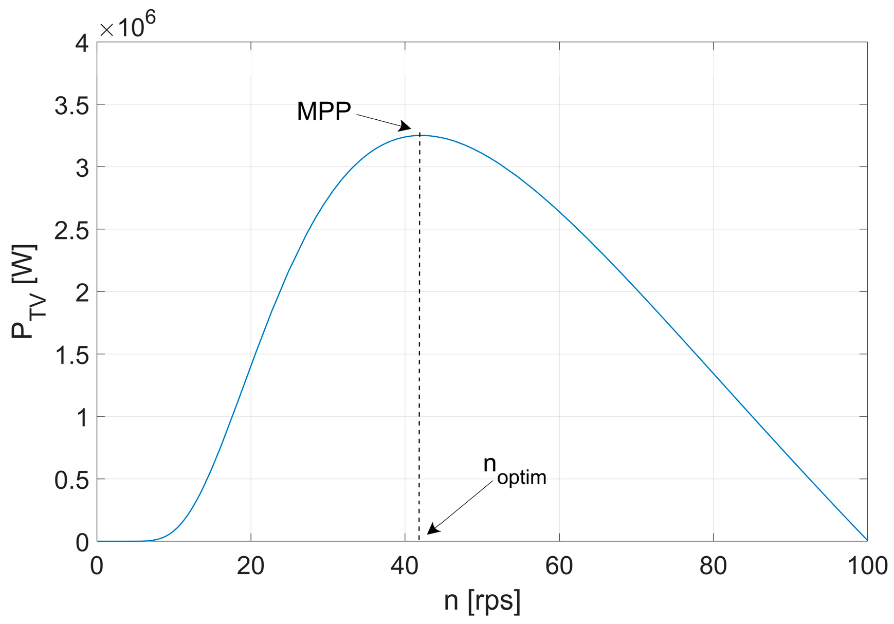
Finally, if $dn/dt$ is measured at any point in time, then from (4) and with the WT operating at $\beta \ne 0$, we could obtain all parameters from $\theta$ simultaneously, via nonlinear regression. A closeup of the $P_{TV}$ curve for $V=11$ [m/s] is revealed in Figure 1 where the MPP corresponds to an optimal MAS value. Although the power curve $P_{TV}$ in Figure 1 is a classical one from the literature, its shape is instrumental in analyzing the dynamic optimal operation behavior. Unstable dynamics observed by linearization at the MPP will challenge how the MPP tracking performance will manifest in response to variable wind speed.

The above MM is critical for deducing optimal operation at various wind speeds [3,4,5,6]. For the WT to operate at MPP, the optimal MAS control is ensured by changing the load at the electric generator, based on wind speed variation [9,10,11,12]. We note another issue with adapting to quick wind speed variation due to the high mechanical inertia of the WT [18,19,20,21,22,42].

2.2. Mathematical Model of the Slip Ring Induction Generator

The Fuhrlander FL-MD-70 models have the following nominal data: equivalent moment of inertia $J=136 \left[\mathrm{k}\mathrm{g}{\mathrm{m}}^2\right]$, nominal power $P_N=P_{GE}=1.5 \left[\mathrm{M}\mathrm{W}\right]$, nominal voltage $U_N=690 \left[\mathrm{V}\right]$, nominal current $I_N=724.64 \left[\mathrm{A}\right]$, pole number equal to four ($2p_1=4$), nominal MAS $n_N=1518.3 \left[\mathrm{r}\mathrm{p}\mathrm{m}\right]$, nominal slip $s_N=-1.2231\times {10}^{-2}$ [24].

The doubly fed slip ring induction wound rotor generator parameters are as follows [43]. The short circuit impedance $Z_{sc}=0.1058 [\Omega ]$, and the short circuit resistance is $R_{sc}=R_s+R_R=4.7610\times {10}^{-2} [\Omega ]$, where $R_S=R_R=2.3805\times {10}^{-2 }[\Omega ]$ are the stator and rotor resistances, respectively. The short circuit nominal reactance is $X_{sc}^n=0.10309 [\Omega ]$ at 50 [Hz], which at different frequencies $f$ becomes $X_{sc}=X_{sc}^n\cdot {\displaystyle \frac{f}{50}}[\Omega ]$. At the stator voltage ${\underset{\_}{U}}_S$ ($\underset{\_}{o}$ means phasor notation for “$o$”) and frequency $f$, the generator stator and rotor currents ${\underset{\_}{I}}_s,{\underset{\_}{I}}_R$ are (at negligible magnetization current)

$$\begin{array}{c}{\underset{\_}{I}}_S={\displaystyle \frac{{\underset{\_}{U}}_S}{R_S+\frac{R_R}{s}+j{X}_{Sc}}}={\displaystyle \frac{{\underset{\_}{U}}_S}{2.3805\times {10}^{-2}+\frac{2.3805\times {10}^{-2}}{s}+j\frac{0.10309f}{50}}},\\ {\underset{\_}{I}}_R=-{\displaystyle \frac{{\underset{\_}{U}}_S}{2.3805\times {10}^{-2}+\frac{2.3805\times {10}^{-2}}{s}+j\frac{0.10309f}{50}}}.\end{array}$$

(5)

where $s$ is the slip at non-nominal operation. Note that the slip depends on the frequency $f$ and MAS value $n$ according to

$$s={\displaystyle \frac{n_1-n}{n1}}={\displaystyle \frac{\frac{f}{p_1}-n}{\frac{f}{p_1}}}={\displaystyle \frac{\frac{f}{2}-n}{f/2}}={\displaystyle \frac{f-2n}{f}}=1-{\displaystyle \frac{2n}{f}},$$

(6)

The generator’s nominal power at the shaft is equivalently expressed as

$$P_{GE}=3{\displaystyle \frac{p_1{U}_S^2(R_R/s)}{{\left(R_S+\frac{R_R}{s}\right)}^2+{\left(2.0618\times {10}^{-3}\right)}^2{f}^2 }},$$

(7)

where $2p_1$ is the number of poles.

With a single stator converter in the generator, wind energy can only be captured within a reduced wind speed domain. Thus, we propose an additional rotor converter within the architecture, which maximizes the wind energy capture over the full interval of wind speeds under which the WT operates. With a wound rotor, the rotor voltage ${\underset{\_}{U}}_R$ can be used to control the desired MAS as follows. Through a rotor converter, it is ${\underset{\_}{U}}_R$ that can change the rotor parameters $R_R$ through an additional additive resistance defined as

$$R_{ad}={\underset{\_}{U}}_R/{\underset{\_}{I}}_R.$$

(8)

Therefore, by proper adaptation of the rotor additional resistance $R_{ad}$, we can change $R_R+R_{ad}$, in turn modifying the equivalent generator’s characteristic to make it depend on the wind speed value $V$. As a consequence, since $R_{ad}$ will be more significant than $R_R$, the rotor electric power $P_{rotor}$ injected into the grid will be approximated with

$$P_{rotor}=3R_{ad}{I}_R^2.$$

(9)

Ultimately, it is the rotor converter that changes $R_{ad}$ through ${\underset{\_}{U}}_R$, to result in $P_{rotor}$. At variable frequency, the asynchronous generator works at the constant stator flux value

$$\Psi ={\displaystyle \frac{U_N}{\omega }}={\displaystyle \frac{U_N}{2\pi f}}={\displaystyle \frac{690}{2\pi 50}}=2.1963 \left[\mathrm{W}\mathrm{b}\right],$$

(10)

at which the “$U/f$” ratio in the stator becomes ${\displaystyle \frac{U_s}{f}}=\Psi \times 2\pi =13.8 [\mathrm{V}\mathrm{s}]$, leading to the final generator power influenced by $R_{ad}$ to be obtained as

$$P_{GE}={\displaystyle \frac{3\times {13.8}^2\times (2.3805\times {10}^{-2}+R_{ad})/(1-2n/f)}{{\left(\frac{2.3805\times {10}^{-2}+(2.3805\times {10}^{-2}+R_{ad})/(1-2n/f)}{f}\right)}^2+{\left(2.0618\times {10}^{-3}\right)}^2 }},$$

(11)

Remark 4. 

With the generator operating at variable frequency, two limitations are imposed:

(1) 

The controlled stator flux has maximal value of $\Psi =2.1963 \left[\mathrm{W}\mathrm{b}\right]$.

(2) 

The stator current $I_s$ is saturated at nominal value $I_N=724.64 \left[\mathrm{A}\right]$.

The wind speed value used to discriminate between the two operating regions being analyzed is $V_{MAX}=10.788$ [m/s] and was obtained by the nonlinear equation system formed with the conditions $P_{TV-MAX}=2442.3V^3=P_{GE}$, plus $I_S=I_N=724.64 \left[\mathrm{A}\right]$, plus the nominal slip condition $1-2n/f=-1.2231\times {10}^{-2}$. Solving the above nonlinear equation leads to $f=101.55$ [Hz], $n=51.394$ [rps] and $V_{MAX}=10.788$ [m/s]. The value $V_{MAX}$ is a threshold between the two operating regions in our work.

Notice that the power converters and the generator have their own internal transient dynamics; however, the time scale is much faster than that of the WT control, so static relationships in terms of current, voltage and power are acceptable.

We briefly underline some critical analysis between induction generators and permanent magnet synchronous ones. Induction generators (with slip rings) have the following advantages. (1) They do not have permanent magnets (PMs), so there will not be failures when the PM demagnetizes. (2) They are generally cheaper compared to synchronous generators with PM. (3) They can very easily switch to motor mode when a quick start of the turbine is desired. Several disadvantages of the induction generators: (1) They cannot provide reactive power. (2) They absorb reactive power from the grid in order to operate.

Synchronous generators with PM have the following advantages. (1) They can provide reactive power. (2) They can operate without voltage from the grid. Some disadvantages include the following. (1) When the PM demagnetizes, they can no longer operate. (2) They require more complex power electronics converters, which may increase the cost and complexity of the system.

3. Wind System Control at Variable Wind Speeds from 3 [m/s] up to ${\mathit{V}}_{\mathit{M}\mathit{A}\mathit{X}}$ [m/s]

With the determined mathematical model of the WT, there are two operation ranges (ORs) under consideration that depend on the wind speed value. The first OR—named OR1—is for $3\le V\left(t\right)\le V_{MAX}=10.788 [\mathrm{m}/\mathrm{s}]$, where the wind power from the WT can still be captured at the generator that works at nominal stator flux and stator current values. Here, the control objective is to regulate the MAS $n$ to the value $n_{OPTIM}$, where the latter depends linearly on the wind speed value $V\left(t\right)$. This control is achievable through the generator frequency $f$. The second OR—called OR2—is for $V_{MAX}\le V\left(t\right)\le 21 [\mathrm{m}/\mathrm{s}]$, where the operation forces the generator power to saturate and the objective is to regulate $P_{TV}$ through the blade pitch angle $\beta$, which will be analyzed later.

For wind speeds up to the value $V_{MAX}$, the MPP must ensure optimal operation for the wind system based on the following equations that define the mechanical Equation (3), considered for the case $\beta =0$ specific to OR1:

$$\begin{array}{c}{P}_{TVMAX}\left(V\right)=2442.3V^3,\\ P_{GE}=-{\displaystyle \frac{571.32\times \frac{\left(2.3805\cdot {10}^{-2}+R_{ad}\right)}{1-\frac{2n}{f}}}{{\left(\frac{2.3805\cdot {10}^{-2}+\frac{\left(2.3805\cdot {10}^{-2}+R_{ad}\right)}{1-\frac{2n}{f}}}{f}\right)}^2+{\left(2.0618\cdot {10}^{-3}\right)}^2}},\\ I_N=724.64\\ ={\displaystyle \frac{13.8}{\sqrt{{\left(\frac{2.3805\cdot {10}^{-2}+\frac{\left(2.3805\cdot {10}^{-2}+R_{ad}\right)}{1-\frac{2n}{f}}}{f}\right)}^2+{\left(2.0618\cdot {10}^{-3}\right)}^2}}},\hfill \\ P_{TV}\left(n,V\right)=5.692\times {10}^5{V}^3{e}^{-{\displaystyle \frac{6.6041V}{n}}}\left(0.15915{\displaystyle \frac{V}{n}}-1.7488\times {10}^{-2}\right)\end{array}$$

(12)

where $P_{TVMAX}\left(V\right)$ is obtained from the MPP on the $P_{TV}\left(n,V\right)$ characteristic, at which point the optimal MAS setpoint is ${n=n}_{OPTIM}=3.8269\times V$.

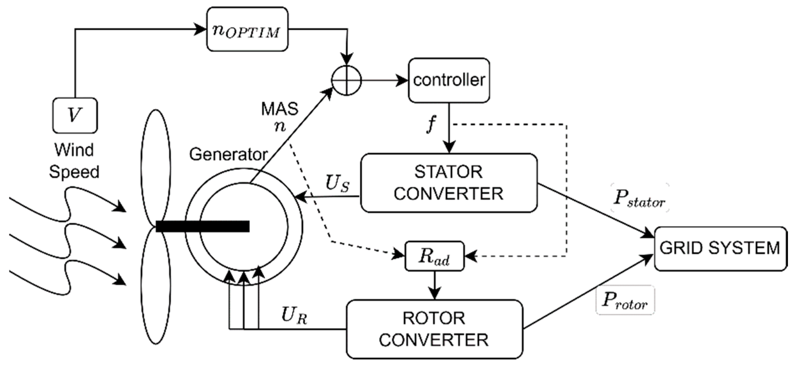
Using the converter block displaced between the generator and the electrical grid, the optimal values of the stator frequency and of the additional rotor resistance $f_{OPTIM}$ and $R_{ad-OPTIM}$ are realized, respectively. From the prescribed ratio “U/f”, the stator voltage $U_S$ follows immediately, with a value that makes the flux constant. The generator’s electrical power $P_{GE}$ injected to the grid is the summed effect of the stator and rotor powers, that is, $P_{GE}=Pstator+Protor$ (see Figure 2).

From a control analysis perspective, the stator current needs to flow at the nominal value $I_N=724.64 \left[\mathrm{A}\right]$ and the MAS $n$ must track the optimal value $n_{OPTIM}$. To smartly decouple the control problem, we extract the solution for $R_{ad}$ that ensures $I_S=I_N$ from the previous equation, which results in $R_{ad}$ as a function of $n$ and $V$:

$$\begin{array}{c}{R}_{ad}(n,V)=R_{ad-OPTIM}(n,V)\\ \hspace{1em}\hspace{1em}\hspace{1em}\hspace{1em}\hspace{1em}\hspace{1em}=\left({\displaystyle \frac{2}{f}}n-1\right)\left(1.8932\times {10}^{-2}f-{\displaystyle \frac{2.3805\times {10}^{-2}}{\frac{2}{f}n-1}}\right)\hfill \\ \hspace{1em}\hspace{1em}\hspace{1em}\hspace{1em}\hspace{1em}\hspace{1em}+2.3805\times {10}^{-2},\hfill \end{array}$$

(13)

Then, the remaining control objective concerns the control of the MAS value $n$ seen as the controlled output, through the stator frequency $f$ seen as the control input. With the resulting values $f,n$, the $R_{ad-OPTIM}$ above ensures nominal stator current value.

3.1. Linearized System Analysis and Control

Equation (3) is transformed to a more common shape under the assumption $\beta =0$, as in

$${\displaystyle \frac{dn}{dt}}={\displaystyle \frac{1}{\overline{J}n}}\left(P_{TV}\left(n,V\right)-P_{GE}\left(n,f\right)\right).$$

(14)

Define $n$ to be a state variable and further rewrite the state space model

$$\begin{array}{c}{\displaystyle \frac{dn\left(t\right)}{dt}}=g\left(n\left(t\right),f\left(t\right),V\left(t\right)\right),\\ y\left(t\right)=h\left(n\left(t\right),f\left(t\right),V\left(t\right)\right)=n\left(t\right),\end{array}$$

(15)

where $g(.)$ is the state equation and $h(.)$ is the output equation. A small signal analysis around a constant operating point is next performed. Let this point be $\mathcal{P}(V_0,n_0,f_0)$. Using the first order linearization around $\mathcal{P}$, we can write

$$\begin{array}{c}{\displaystyle \frac{d\Delta n\left(t\right)}{dt}}={\left.{\nabla }_{n}g\right|}_{V_0,n_0,f_0}\Delta n+{\left.{\nabla }_{f}g\right|}_{V_0,n_0,f_0}\Delta f+{\left.{\nabla }_{V}g\right|}_{V_0,n_0,f_0}\Delta V,\\ \Delta y\left(t\right)={\left.{\nabla }_{n}h\right|}_{V_0,n_0,f_0}\Delta n+{\left.{\nabla }_{f}h\right|}_{V_0,n_0,f_0}\Delta f+{\left.{\nabla }_{V}h\right|}_{V_0,n_0,f_0}\Delta V=\Delta n\left(t\right),\end{array}$$

(16)

where we denote with $\nabla$ the Jacobian of the functions $g,h$ with respect to their arguments at the operating point $\mathcal{P}(V_0,n_0,f_0)$ and $\Delta$ means the small variation of the argument about the linearization value. Subsequently, the variation notation with $\Delta$ will be discarded and we use only absolute notation $f,V,n$. The variables’ roles are as follows. $f$ is the control input, $V$ is the disturbance input, $n$ is the control output. In the Laplace transform domain of the variable “s”, the following transfer functions result: $H_{f\to n}\left(s\right)=K_f/(1+sT)$ and $H_{V\to n}\left(s\right)=K_v/(1+sT)$.

Remark 5. 

Linearization around several points $\mathcal{P}(V_0, n_0, f_0)$ reveals crucial observations that have critical impact upon the control design. We classify two main cases:

• Case 1. When linearization is performed at the MPP by imposing the operating point constraint $n_0=3.8269f_0$, we obtain that $K_f>0,K_v<0$ and $T<0$.
• Case 2. When the linearization is performed at arbitrary point $\mathcal{P}(V_0,n_0,f_0)$ , we observe the following. (a) When $n_0>3.8269f_0$ (operation to the right of the MPPT on the $P_{TV}$ curve), we have $K_f<0,K_v>0$ and $T>0$ , making for an open-loop stable transfer function; (b) when $n_0<3.8269f_0$ (operation to the left of the MPPT on the $P_{TV}$ curve), we have $K_f>0,K_v<0$ and $T<0$ , making for an open-loop unstable transfer function.

With the nonlinear process as the one in (12), there are several tradeoffs to be accounted for, when linear control is to be used: robustness under the time varying process nature, stability and performance. When operating at variable wind speeds, the design choices become more stringent. For a reasonable ramp-like variation of the wind speed value $V\left(t\right)$, a double integrator should be included in the controller (according to the internal model principle); however, this reduces the stability margin. Two options are considered:

Option (1) The feedback controller is a proportional–integral (PI) controller with the transfer function $C\left(s\right)=(p_{1}s+p_0)/s$. With the closed-loop transfer function from MAS setpoint, the controlled MAS is $(K_f{p}_{1}s+K_f{p}_0)/\left(T{s}^2+\left(1+K_f{p}_1\right)s+K_f p_0\right)$ with the characteristic polynomial of the closed loop being $T{s}^2+\left(1+K_f{p}_1\right)s+K_f p_0$, which allows for flexible and robust design. However, there will be nonzero steady state tracking error with respect to ramp-like disturbance $V\left(t\right)$ as well as for ramp-like MAS reference input imposed by $V\left(t\right)$ via linear dependence, based on the MPP principle. For both Case 1 and Case 2b in Remark 5, there exist negative values of $p_1<0,p_0<0$ that will make the closed loop stable. For Case 2a in Remark 5, again, a suitable combination of $p_1,p_0$ can be found to stabilize the closed loop.

Option (2) The feedback controller is a double integrator with transfer function $C\left(s\right)=(p_{1}s+p_0)/s^2$. The closed-loop characteristic polynomial will be $T{s}^3+s^2+K_f{p}_{1}s+K_f{p}_0$ which may still offer stability for proper choice of $p_1,p_0$, but stability margin is significantly smaller. In this case, since the coefficient of $s^2$ is 1, then for $T<0$ (Cases 1 and 2b from Remark 5), it will be impossible to make a stable closed loop by any selection of $p_1,p_0$. We conclude that a double integrator is not feasible to be designed at the MPP; however, it may be designed at a suboptimal operating point such as in Case 2a in Remark 5.

We consider a reasonable ramp-like variation for the wind speed as in $V\left(t\right)=2.0071\times {10}^{-3}t+3$, starting from $V\left(0\right)=3 [{\displaystyle \frac{\mathrm{m}}{\mathrm{s}}}]$ and up to the value $V_{MAX}$. After extensive testing with selected pair values $(p_1,p_0)$ that make the closed loop stable around the linearization point, when testing in dynamic regime for the ramp-like $V\left(t\right)$, only marginally stable control is achieved. This motivates the selection of the plain PI control algorithm revealed under Option 1, which will drive the control to be stable, fast and with acceptable steady state tracking error. For the operating point characterized by $\mathcal{P}(V_0=4 [\mathrm{m}/\mathrm{s}],n_0=15.30 [\mathrm{r}\mathrm{p}\mathrm{s}],f_0=0.953 [\mathrm{H}\mathrm{z}\left]\right)$, we select $p_1=-10, p_0=-30$ as the PI controller gain parameters leading to $C_{PI}\left(s\right)=-(10s+30)/s$.

3.2. A Competitive Linear VRFT Controller for Nonlinear Control

For comparison, we design a competitive PI controller algorithm based on the VRFT principle [44,45,46,47,48,49] which was proposed for automated tuning based on (but not limited to) reference model specification. For data collection, we fix the wind speed value $V=5$ [m/s] and use a pre-stabilizing feedback controller with transfer function $-20-0.2/s$ applied to the closed-loop error $e\left(t\right)=n_{ref}\left(t\right)-n\left(t\right)$. 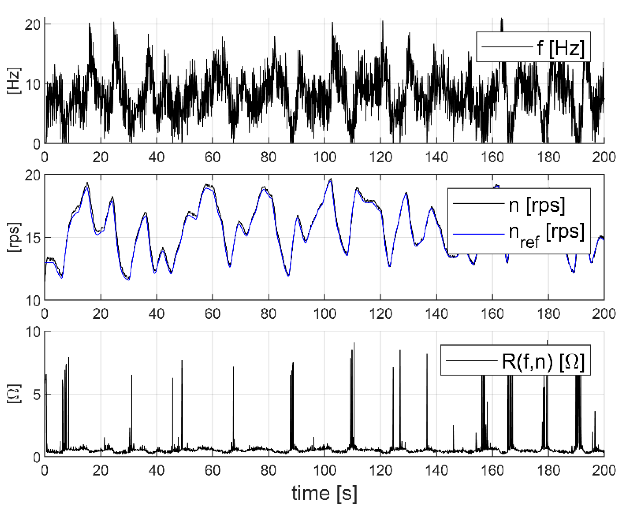Here, $11\le n_{ref}\le 20$ [rps] is generated as piece-wise constant uniform random samples with periodic switching at 3 [s] additionally filtered with a lowpass second-order filter with function $1/(s^2+2s+1)$. The control input $f$ is saturated below at zero and it is further excited with a wide power spectrum uniform random noise with amplitude in $[-4;4]$ with period 0.1 [s]. The collected input $f$ and controlled output $n$ are recorded at a sampling period of $T_s=0.05$ [s] and are shown in Figure 3. The tuned PI controller is to be implemented in discrete time; thus, it is parameterized as $C_{PI}^{VRFT}\left(q\right)=(p_0+p_1{q}^{-1})/(1-q^{-1})$. Here, $q$ is the discrete-time single step forward operator, analogous to the $z$ operator.

The reference model for setting up the desired behavior from $n_{ref}$ to $n$ in closed loop is picked as $M\left(s\right)={10}^2/(s^2+2\cdot 0.9\cdot 10\cdot s+{10}^2)$ and discretized accordingly at $T_s=0.05$ [s], to reach $M\left(q\right)$ discrete-time representation. Let the dataset of input–output samples be $DS=\{f_k,n_k\}$ with sample index $1\le k\le N$, where in our case study, we measured $N=4000$ sample points. A discrete-time VRFT prefilter is a common option for filtering the virtual feedback error defined as $e_k^v=M^{-1}\left(q\right)n_k-n_k$ and also for filtering $f_k$. This prefilter used in our case is set to $0.8/(1-0.2q^{-1})$ with sampled period $T_s$. The loss function to be minimized is $L_{VRFT}=1/N{\sum }_{k=1}^N{\left(f_k-C_{PI}^{VRFT}\left(q\right)e_k^v\right)}^2$. The resulting identified controller is $C_{PI}^{VRFT}\left(q\right)=(-4.0534+0.6495q^{-1})/(1-q^{-1})$.

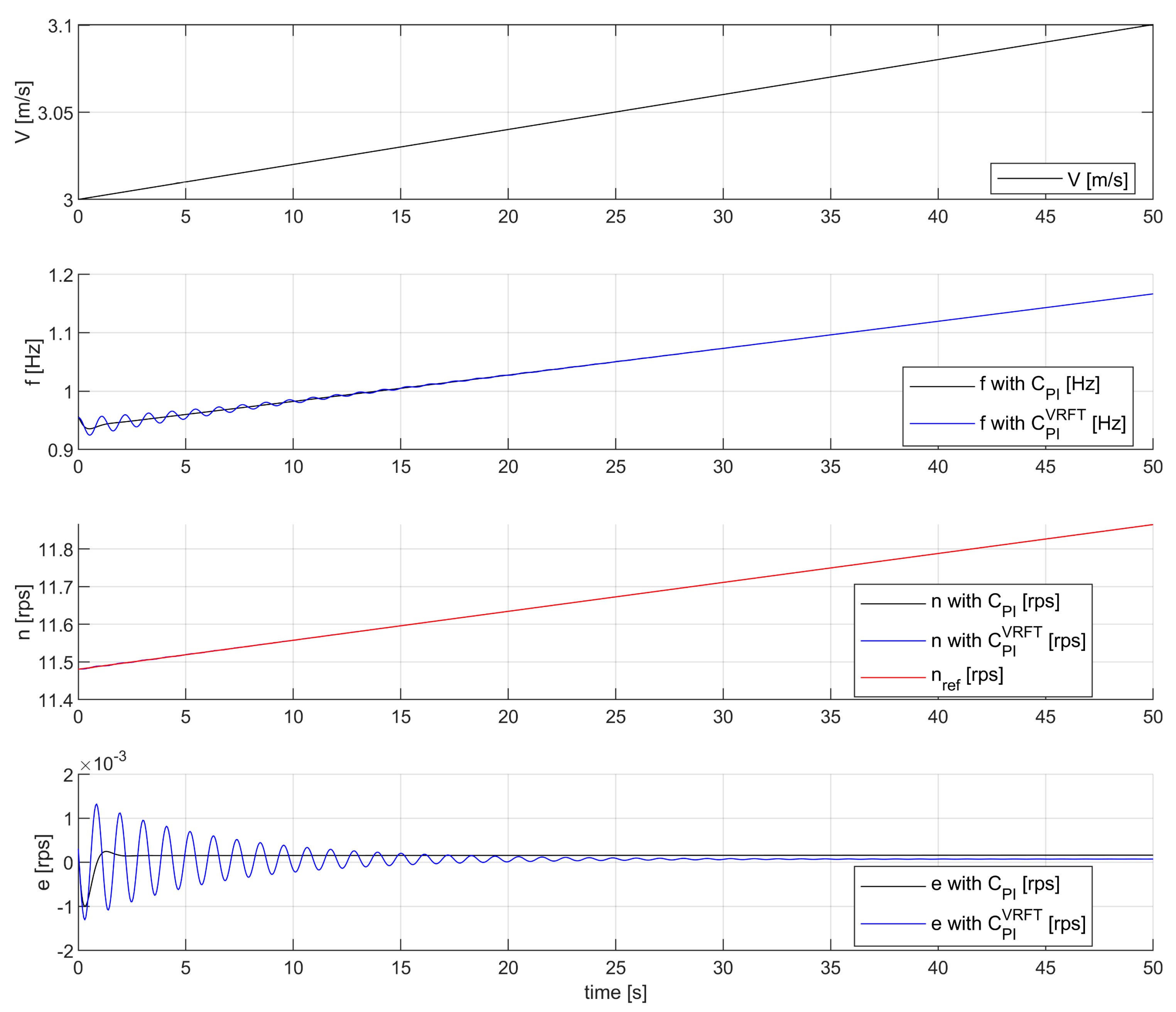
Comparative control results obtained with $C_{PI}\left(s\right)$ and $C_{PI}^{VRFT}\left(s\right)$ (the latter being implemented in discrete time) are offered in Figure 4. Note that in the testing phase, $V\left(t\right)=3+2.0071\times {10}^{-3}t$, and it acts, as a parametric disturbance on the model $P_{TV}$ but also imposes the setpoint as ${n_{ref}=n}_{OPTIM}=3.8269\times V$. Initial conditions for the test scenario are set as $f_0=0.953 \left[\mathrm{H}\mathrm{z}\right],n_0=11.481 \left[\mathrm{r}\mathrm{p}\mathrm{s}\right]$.

We observe the following. Acceptable tracking control is obtained with respect to $n_{ref}$ and relatively small steady-state errors are visible with respect to the ramp-like $V\left(t\right)$. We stress that the underlying process is nonlinear time-varying due to the parameter $V\left(t\right)$ acting as disturbance but also imposing the MPP operation via $n_{OPTIM}$. Surprisingly, given the oscillatory nature of the transient response obtained with the VRFT-trained PI controller, it shows a reduced steady-state tracking error under time-varying $V\left(t\right)$, when compared with the simple PI controller.

Regarding the sensitivity of the design with respect to the parameter’s choice, the VRFT controller seemed very sensitive to the choice of the reference model bandwidth. There may be several reasons for it, namely the linear VRFT formulation needing to cope with the nonlinear system, although the collected data span quite a wide range near the operating point, thus not perfectly fitting a linear process model description. We underline that the data collection is performed on the nonlinear model, although the linearity assumptions about the method were enforced. Secondly, the time-varying nature of the process due to the wind speed value is another important factor affecting the hypothesis.

On the other hand, the linear PI controller has fewer design parameters, namely the proportional and integrator gains, and we could observe larger domain of values under which the closed loop was stable. We aimed for two criteria, in this order: (1) fast transient response, and (2) as small as possible steady-state error with respect to the ramp-like wind speed variation. The PI controller served as a baseline for performance, while the VRFT one was tuned (via the method hyperparameters) to outperform this behavior. The achieved compromise for a stable design was met by smaller steady-state tracking errors, with larger oscillations in the initial transients.

4. Wind System Control at Variable Wind Speeds from ${\mathit{V}}_{\mathit{M}\mathit{A}\mathit{X}}$ [m/s] up to 21 [m/s]

In the region OR2 where $V_{MAX}\le V\left(t\right)\le 21$ [m/s], the reliable WT operation requires the generator power to saturate, and the objective is to regulate $P_{TV}$ via the blade pitch angle $\beta$. The control process unfolds as follows. Firstly, the values of $f$ and $R_{ad}$ are calculated at $V_{MAX}$, assuming constant steady state optimal MPP operation. In this case, the optimal MAS will be $n_{OPTIM}=3.8269\times V_{MAX}=3.8269\times 10.788=41.285 \left[\mathrm{r}\mathrm{p}\mathrm{s}\right]$. Two conditions are used to saturate the generator power, namely $P_{GE}=1.5\times {10}^6$ [W] and $I_S=I_N=724.64$ [A]. The following nonlinear system of equations:

$$\begin{array}{c}{P}_{GE}=-{\displaystyle \frac{571.32\times \frac{\left(2.3805\cdot {10}^{-2}+R\right)}{1-\frac{2n}{f}}}{{\left(\frac{2.3805\cdot {10}^{-2}+\frac{\left(2.3805\cdot {10}^{-2}+R\right)}{1-\frac{2n}{f}}}{f}\right)}^2+{\left(2.0618\cdot {10}^{-3}\right)}^2}},\\ I_N=724.64={\displaystyle \frac{13.8}{\sqrt{{\left(\frac{2.3805\cdot {10}^{-2}+\frac{\left(2.3805\cdot {10}^{-2}+R\right)}{1-\frac{2n}{f}}}{f}\right)}^2+{\left(2.0618\cdot {10}^{-3}\right)}^2}}},\end{array}$$

(17)

is used for the value ${n=n}_{OPTIM}=41.285$ [rps] to solve for stator frequency $f^{*}=49.038$ [Hz] and for the additional rotor resistance $R_{ad-OPTIM}=0.6273 [\Omega ]$ that saturate $P_{GE}$ to the maximal value of 1.5 [MW]. Under this consideration, with fixed values for $f=f^{*}$ and $R_{ad}=R_{ad-OPTIM}$, we are left with $P_{GE}={\displaystyle \frac{371.99}{\left[{\left(\frac{1.3278\cdot {10}^{-2}}{4.0785\times {10}^{-2}n-1}-4.8544\times {10}^{-4}\right)}^2+4.251\times {10}^{-6}\right]\left(4.0785\times {10}^{-2}n-1\right)}}$, which only depends on the MAS value $n$. The dynamical system is now

$$\begin{array}{c}{\displaystyle \frac{dn}{dt}}={\displaystyle \frac{1}{\overline{J}n}}\left(P_{TV}\left(n,V,\beta \right)-P_{GE}\left(n\right)\right),\\ P_{TV}\left(n,V,\beta \right)=5.692\times {10}^5{V}^3{e}^{-{\displaystyle \frac{6.6041V}{n}}}\left(0.15915{\displaystyle \frac{V}{n}}{e}^{-3.0303\times {10}^{-2}\times \beta }-1.7488\times {10}^{-2}\right),\\ P_{GE}={\displaystyle \frac{371.99}{\left[{\left(\frac{1.3278\cdot {10}^{-2}}{4.0785\times {10}^{-2}n-1}-4.8544\times {10}^{-4}\right)}^2+4.251\times {10}^{-6}\right]\left(4.0785\times {10}^{-2}n-1\right)}},\end{array}$$

(18)

which is ready to be used for control purposes. Next, the control analysis and design are attempted within region OR2.

4.1. Linearized System Analysis and Control

We bring the dynamical system (18) again to a controllable object form where

$$\begin{array}{c}{\displaystyle \frac{dn\left(t\right)}{dt}}=g\left(n\left(t\right),V\left(t\right),\beta \left(t\right)\right),\\ y\left(t\right)=h\left(n\left(t\right),V\left(t\right),\beta \left(t\right)\right)=P_{TV}(n,V,\beta ),\end{array}$$

(19)

and now the control objective is to regulate $P_{TV}$ at the setpoint $P_{TV}^{*}=1.5$ [MW] using the blade pitch angle $\beta \left(t\right)$ as the control input variable. Let us consider again a linearization point $\mathcal{P}(V_0=V_{MAX},n_0=3.8269\times V_0,{\beta }_0=0)$ to reflect operation near the MPP. Using the first-order linearization around $\mathcal{P}$, we can write

$$\begin{array}{c}{\displaystyle \frac{d\Delta n\left(t\right)}{dt}}={\left.{\displaystyle \frac{dg}{dn}}\right|}_{V_0,n_0,{\beta }_0}\Delta n+{\left.{\displaystyle \frac{dg}{df}}\right|}_{V_0,n_0,{\beta }_0}\Delta \beta +{\left.{\displaystyle \frac{dg}{dV}}\right|}_{V_0,n_0,{\beta }_0}\Delta V,\\ \Delta y\left(t\right)={\left.{\displaystyle \frac{dh}{dn}}\right|}_{V_0,n_0,{\beta }_0}\Delta n+{\left.{\displaystyle \frac{dh}{df}}\right|}_{V_0,n_0,{\beta }_0}\Delta \beta +{\left.{\displaystyle \frac{dh}{dV}}\right|}_{V_0,n_0,{\beta }_0}\Delta V=\Delta n(t),\end{array}$$

(20)

where we obtain the Jacobian of the functions $g,h$ with respect to their arguments at the operating point $\mathcal{P}(V_0,n_0,{\beta }_0)$ and $\Delta$ means the small variation of the argument about the linearization value. The transfer functions that result are $H_{\beta \to P_{TV}}\left(s\right)=-1.603\times {10}^5(1.70716s+1)/(1.70719s+1)$ and $H_{V\to P_{TV}}\left(s\right)=8.527\times {10}^5(1.70716s+1)/(1.70719s+1)$. Notice that the numerator and denominator time constants are only slightly different in both cases; therefore, pole-zero cancellation is safely employed, which means that in the linearized model, we write $P_{TV}\left(s\right)=k_{\beta }\beta \left(s\right)+k_{V}V\left(s\right)$, which renders the process a static one. Of course, the underlying system is nonlinear time-varying and the values $k_{\beta },k_V$ will change with the operating point.

The role of $V\left(t\right)$ will be important, since it will be modeled as a ramp-like disturbance. This time, different from OR1, the control goal will not be MPP tracking (which adapts $n_{OPTIM}$ based on $V$) but the WT operation imposed by regulating $P_{TV}$ at the setpoint of $P_{TV}^{*}\left(t\right)=$ 1.5 [MW]. In this context, the control must be designed so as to deliver both reference tracking and disturbance rejection. With the underlying analyzed process transfer function, a straightforward option is to use a double integrator feedback controller on the feedback error $e\left(t\right)=P_{TV}^{*}(t)-P_{TV}(t)$, namely $C\left(s\right)=(p_{1}s+p_0)/s^2$.

4.2. A Nonlinear Sliding Mode Controller

For a sliding mode control algorithm design [50,51,52], the dynamical system (18), (19) is transformed to input affine form. First, let

$$\dot{y}\left(t\right)={\nabla }_{n}h\cdot \dot{n}+{\nabla }_{V}h\cdot \dot{V}+{\nabla }_{\beta }\dot{\beta },$$

(21)

with ${\nabla }_{n}h={\displaystyle \frac{dh\left(n,V,\beta \right)}{dn}},{\nabla }_{V}h={\displaystyle \frac{dh\left(n,V,\beta \right)}{dV}},{\nabla }_{\beta }h={\displaystyle \frac{dh(n,V,\beta )}{d\beta }}$ and let us augment the dynamical system with the integrator $\dot{\beta }=u$. Then, use the MAS equation $\dot{n}={\displaystyle \frac{1}{\overline{J}n}}(y-P_{GE}(n))$ to further arrive at

$$\begin{array}{c}\dot{y}={\displaystyle \frac{{\nabla }_{n}h}{\overline{J}n}}y+{\nabla }_{\beta }h\cdot u+{\nabla }_{V}h\cdot V-{\displaystyle \frac{{\nabla }_{n}h}{Jn}}{P}_{GE}\\ \hspace{1em}\hspace{1em}\hspace{1em}\hspace{1em}\hspace{1em}\hspace{1em}:=\phi \left(n,V,\beta \right)\cdot y+B\left(n,V,\beta \right)\cdot u+\sigma (n,V,\beta ),\hfill \end{array}$$

(22)

where $\phi \left(n,V,\beta \right):={\displaystyle \frac{{\nabla }_{n}h}{\overline{J}n}}$ is the output multiplicative factor in the output differential equation, $B\left(n,V,\beta \right):={\nabla }_{\beta }h$ is the input multiplicative factor and $\sigma \left(n,V,\beta \right):={\nabla }_{V}h\cdot V-{\displaystyle \frac{{\nabla }_{n}h}{Jn}}\cdot P_{GE}(n)$ is the uncertainty factor.

Assumption 1. 

The input multiplicative factor $B\left(n,V,\beta \right)$ and its reciprocal 1/$B\left(n,V,\beta \right)$ are well defined within the entire operating region OR2.

Assumption 2. 

The uncertainty factor $\sigma (n,V,\beta )$ is bounded within the operating region OR2. Let this bound $\overline{\sigma }$ satisfy $\left|\sigma \right|<\overline{\sigma }$.

Remark 6. 

Normally, the uncertainty term $\sigma$ is partially measurable since its expression is well defined and all arguments $n,V,\beta$ are measurable. However, original model uncertainty, parameter aging and unmodeled dynamics will be lumped inside this term altogether. Take, e.g., $\phi +\widehat{\phi }$ and $B+\widehat{B}$ as additive uncertainties about nominal values $\phi , B$, then $\widehat{\phi }y+\widehat{B}u$ could easily be lumped inside $\sigma$. Both Assumption 1 and Assumption 2 are very reasonable and hold for quite wide operating conditions.

Let the following controller be used:

$$u=B^{-1}\left({\dot{y}}^{*}-\phi y\right)-B^{-1}Ksgn\left(g\right),$$

(23)

where $g:=e$ is the switching variable, which is also the control error $e=y-y^{*}$ for $y^{*}=P_{TV}^{*}$, a reference input. In the proposed control law, $K>0$ is a design gain. The factor $B^{-1}\left({\dot{y}}^{*}-\phi y\right)$ is the equivalent control component and $B^{-1}Ksgn\left(g\right)$ is called the switching component. The most direct stability analysis can be formalized with the next theorem.

Theorem 1. 

The control system obtained by the output Equation (22) coupled with controller (23) is stable for $K>\overline{\sigma }$.

Proof of Theorem 1. 

Substitute $u$ from (23) in (22) and we obtain $\dot{y}={\dot{y}}^{*}-Ksgn\left(g\right)+\sigma$, which is equivalent to $\dot{g}=-Ksgn\left(g\right)+\sigma$.

• Define the Lyapunov function $V\left(g\right)=0.5g^2$ and calculate $\dot{V}=g\dot{g}$.
• Case (1) When $g>0$, $sgn\left(g\right)=1$ and $\dot{g}=-K+\sigma \le -K+\overline{\sigma }<0$, which makes $\dot{V}=g\dot{g}<0$.
• Case (2) When $g<0, sgn\left(g\right)=-1$ and $\dot{g}=K+\sigma \ge K-\overline{\sigma }>0$, which makes $\dot{V}=g\dot{g}<0$.
• Based on the two cases above, from the fact that $g:=e$ and $e=y-y^{*}$ depends on bounded $y^{*}$ and on $y$, the control system is Lyapunov-stable with bounded $y$. □

Remark 7. 

The upper bound $\overline{\sigma }$ may be estimated more or less accurately in practice. It is customary to choose a large enough $K>\overline{\sigma }$ to allow for a safe robustness margin. The advantage with respect to the linear double integral controller is the stability certification.

Remark 8. 

Although the proposed control draws inspiration from the sliding mode method, it is seen as a particular type of sliding mode, as explained next. For one, the equivalent control component $B^{-1}\left({\dot{y}}^{*}-\phi y\right)$ found within the control law, does not compensate for some nominal value $\sigma$ of the uncertainty. In other words, the equivalent control $B^{-1}\left({\dot{y}}^{*}-\phi y\right)$ is constructed for an equivalent null uncertainty. As a consequence, it will make the control forever chatter in a limited bandwidth around $g=0$, to be analyzed next. Secondarily, the sliding motion is missing, i.e., the proposed controller consists only of the reaching phase, as it follows from the definition of $g:=e$. This way, the control may be seen as a discontinuous switching one, where the factor $-B^{-1}Ksgn\left(g\right)$ is introduced exactly to compensate for the uncertainty. The control is thus formulated directly as a tracking objective. We can gain deeper insight into the control behavior as follows.

• First, notice that $\dot{V}=g\dot{g}=g\left(-Ksgn\left(g\right)+\sigma \right)=-K\left|g\right|+g\sigma$. Since $\left|g\sigma \right|\le \left|g\right| \overline{\sigma }$, we find that $\dot{V}\le -K\left|g\right|+\overline{\sigma }\left|g\right|=(-K+\overline{\sigma })\left|g\right|$, which makes $\dot{V}<0$ bounded away from zero for all $g\ne 0$ and $K>\overline{\sigma }$. When $g=0$, we notice that $\dot{g}=\sigma \ne 0$, which means that the surface $g=0$ is not invariant and the trajectory will bounce back to a vicinity of $g=0$ from where the switching component will again push it towards $g=0$. This will make the system permanently chatter around $g=e=0$, and therefore, $y$ will oscillate around $y^{*}$ within an acceptable boundary layer. Also, a finite reaching time of $g=0,$ starting from an initial condition $g\left(t_0\right)$, is measured (by integration) to be less than ${\displaystyle \frac{\left|g\left(t_0\right)\right|}{K-\overline{\sigma }}}$.
• When the control implementation is digitalized, the sampling delay introduces chattering irrespective of how is $K$ selected about $\overline{\sigma }.$ With existing smooth implementations of the switching function $sgn(.)$ , chattering is reduced but not completely removed. Generally, a good practical compromise can be achieved for proper selection of $K$ , and we note that there exists a major advantage, since $\sigma$ is considered completely unknown; hence, it does not require recalculation for it to be compensated. Should a reliable estimate of $\sigma$ be plugged in (23), a smaller $K$ will reduce the chattering further.

4.3. A Model Predictive Adaptive Controller

A model predictive adaptive controller (MPAC) is next designed [53,54,55,56,57,58,59], starting from the linearized model $P_{TV}\left(s\right)=k_{\beta }\beta \left(s\right)+k_{V}V\left(s\right)$. The design is carried out with respect to the input channel $\beta$, thus ignoring the effect of $V$ directly; however, for model uncertainty and disturbance rejections, we augment the control input channel with an integrator. Hence, the augmented model for MPAC design becomes $P_{TV}\left(s\right)={\displaystyle \frac{k_{\beta }}{s}} {\beta }^{\prime }\left(s\right)$, with ${\beta }^{\prime }$ the control input derivative. We discretize the model using the zero-order hold method and arrive at

$$P_{TV,k}=P_{TV,k-1}+k_{\beta }{T}_s{{\beta }^{\prime }}_k=P_{TV,k-1}+k_d{\beta }_k^{\prime },$$

(24)

which incorporates the sampling period $T_s$. Let the output predictors ${\widehat{P}}_{TV,k+i},i=1,\dots ,N$ be unfolded over time as

$$\left(\begin{array}{c}{\widehat{P}}_{TV,k+1}\\ {\widehat{P}}_{TV,k+2}\\ ⋮\\ {\widehat{P}}_{TV,k+N}\end{array}\right)=\left(\begin{array}{c}{P}_{TV,k}\\ P_{TV,k}\\ ⋮\\ P_{TV,k}\end{array}\right)+\left(\begin{array}{cccc}{k}_d& 0& \dots & 0\\ k_d& k_d& \dots & 0\\ ⋮& ⋮& \ddots & ⋮\\ k_d& k_d& \dots & k_d\end{array}\right)\left(\begin{array}{c}{\beta }_k^{\prime }\\ {\beta }_{k+1}^{\prime }\\ ⋮\\ {\beta }_{k+N-1}^{\prime }\end{array}\right)\leftrightarrow {\widehat{\mathrm{P}}}_{\mathrm{T}\mathrm{V}}=\Psi +P{\rm B},$$

(25)

where the ${\widehat{P}}_{TV}$ vector stacks the future outputs, the $\Psi$ vector is the current state context and ${\rm B}={\left[{\beta }_k^{\prime },\dots ,{\beta }_{k+N-1^{\prime }}\right]}^T$ stacks the present and future control input derivatives, $P$ is the input predictor matrix. Define the receding horizon cost

$$J\left(k\right)=\sum _{i=1}^N{\left(r_{k+i}-{\widehat{P}}_{TV,k+i}\right)}^2+\lambda {\left({\beta }_{k+i-1}^{\prime }\right)}^2={\left(R-{\widehat{P}}_{TV}\right)}^T\left(R-{\widehat{P}}_{TV}\right)+\lambda {{\rm B}}^T{\rm B},$$

(26)

where $R={\left[r_{k+1},\dots ,r_{k+N}\right]}^T$ stacks the future reference inputs and $\lambda$ is a control energy/effort penalty. The cost is written as $J\left(k\right)={{\rm B}}^T\left(P^{T}P+\lambda I\right){\rm B}-2M^{T}P{\rm B}+M^{T}M$ with $M=R-\Psi$ and $I$ the identity matrix of appropriate size. Define the inequality type constraints ${\beta }_{min}\le {\beta }_{k+i}^{\prime }<{\beta }_{max},i=1,\dots N-1$ and rewrite in matrix form as

$$\left(\begin{array}{c}I\\ -I\end{array}\right){\rm B}\le \left(\begin{array}{c}{{\rm B}}_{max}\\ -{{\rm B}}_{min}\end{array}\right),$$

(27)

where ${{\rm B}}_{max}={\left[{\beta }_{max},\dots ,{\beta }_{max}\right]}^T\in {\mathbb{R}}^N,{{\rm B}}_{min}={\left[{\beta }_{min},\dots ,{\beta }_{min}\right]}^T\in {\mathbb{R}}^N$ capture the upper and lower bound constraints on the control input derivative, in linear form. A more compact form of the linear constraints in the input is $A{\rm B}\le N, A=\left(\begin{array}{c}I\\ -I\end{array}\right), N=\left(\begin{array}{c}{{\rm B}}_{max}\\ -{{\rm B}}_{min}\end{array}\right)$. The MPAC control algorithm is finally expressed as

$${{\rm B}}^{\mathrm{*}}=\arg \underset{{\rm B}}{\min }J\left(k\right), s.t. A{\rm B}\le N,$$

(28)

and it is solved as a convex quadratic optimizer, benefiting the inherent favorable structure of the problem. In general, in MPAC for nonlinear systems where the problem structure cannot be exploited, other numerical-based search algorithms must be used [60,61]. Based on the receding horizon principle, only the first component of ${\rm B}$ is extracted and next sent to the plant for actuation, i.e., ${\beta }_k^{\prime }={\rm B}\left(1\right)$, and that implies numerical integration through the artificial integrator augmenting the plant model in the first place.

Notice that in the MPAC, the parameter $k_{\beta }$ adapts online with the current linearization point, and hence, it triggers the online update of $k_d$ and of the matrix $P$. The matrix $\Psi$ is updated online based on the last controlled output. Parameter $\lambda$ acts as a regularizer that trades off fast response time and robustness against uncertainty and disturbances. The input control constraints also act as regularizers with a similar effect; hence, more hyperparameters lead to more flexibility in the design. The artificial integrator augmenting the base dynamics adds another level of robustness.

4.4. Testing the Controllers Designed for OR2

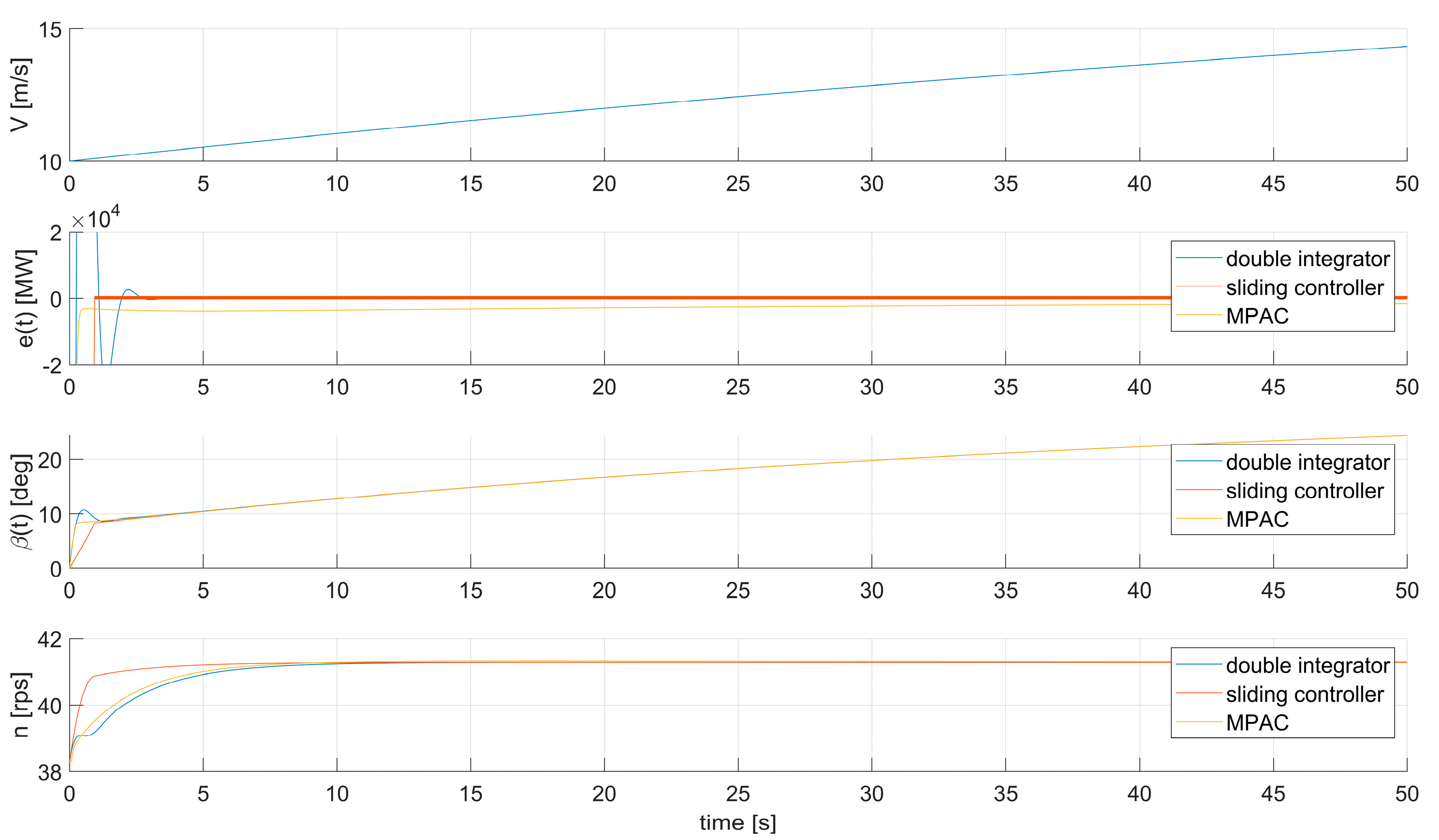
The test scenario for the competitive controllers designed for the region OR2 is captured by a wind speed variation $V\left(t\right)=21-11e^{-0.01t}$, initial conditions at time $t=0$ are $V_0=10$ [m/s] (close to $V_{MAX}$ but rounded to a smaller integer value, without generality loss), $n_0=38.269$ [rps], ${\beta }_0=0 \left[\mathrm{d}\mathrm{e}\mathrm{g}\right]$ and $P_{TV0}=2.4423$ [MW]. For time intervals up to several tens of seconds, the variation of $V\left(t\right)$ can be considered ramp-like, as will be apparent from the plots.

For robustness, the poles of the closed loops of the linearized system with the double integrator controller are allocated, resulting in $p_1=-5,{ p}_0=-20$.

For the sliding mode controller, the main parameter is chosen as $K={10}^6$, and for chattering reduction, the sign function in the controller switching is smoothed as $sgn\left(g\right)=\tanh \left(10g\right)$.

For MPAC application, we choose $N=3$; the blade pitch angle derivative was saturated within thresholds ${\beta }_{min}=-40,{ \beta }_{max}=40$, and the control effort on the pitch angle derivative was set to $\lambda =1$. An interior-point barrier optimizer was employed. A sample period of $T_s=0.05$ [s] was used, as with the VRFT discrete-time controller.

The control results measured with all proposed controllers are visible in Figure 5. Fast transient responses are obtained with a slight advantage for the sliding mode controller. In the disturbance rejection, the linear double integrator rejects the disturbance with steady-state tracking error close to zero, similarly to the sliding mode controller. This is surprising, as the double integrator is linear; however, it displays sufficient robustness. The MPAC controller displays decreasing steady-state tracking error at a slower pace.

The control in operating region OR2 is deemed feasible and performant with the proposed controllers. That is, reliable operation follows by regulating $P_{TV}\left(t\right)$ to the desired value $P_{TV}^{*}\left(t\right)=1.5$ [MW]. Chattering with $\beta \left(t\right)$ is not seen due to its small value; however, its indirect effect is observed with the sliding mode controller, even though the computed $u\left(t\right)$ is integrated once to arrive at $\beta \left(t\right)$. The results were tested on the entire wind speed variation domain [10; 21] [m/s] and they hold the same control behavior. Due to the fast-transient responses, only the first 50 s are presented in Figure 5. Due to its simplicity and ability to simultaneously reject disturbance and track the reference, the double integrator may be the best tradeoff. However, testing the robustness in extreme conditions under additional operational constraints may leave a significant space for either the sliding-mode controller or for the MPAC one.

Regarding the sensitivity of the compared controllers with respect to the parameter’s choice, we disclose the following. The linear double integrator provided the baseline performance, with two main criteria, in this order: (1) fast transient response and (2) null steady-state tracking error with respect to the ramp-like wind speed.

For the sliding mode controller, we expected to outperform the linear double integrator; however, we could not make the transient response much faster, since the chattering increased. Notice from the theoretical design that the chattering will be present under any circumstance, since we chose to not compensate explicitly for the uncertainty; thus, we leave it to the switching component to deal with it. This way, the resulting controller has much simpler expression and does not need to evaluate the uncertainty factor $\sigma$ at each integration time step, so the computational complexity is heavily reduced. With the chattering result, as seen in the plot, the performance was considered good enough, with zero-on-average steady-state tracking error.

For the MPAC controller, although the targeted performance was better than with the linear double integrator, we notice its apparent lower performance when compared with the double integrator. It manifests a significantly longer time needed to bring the tracking error to zero, although the response is similarly fast to the linear controller. There are two advantages, however, to the MPAC controller. The first one is that it only has a single integrator, like the sliding mode controller. The second one is the ability to approach constraints on the controlled variables, which is a unique feature when compared with the other two competitive controllers. Although not visible in the tested scenario, the transient response obtained with MPAC could have been faster, given that the thresholds ${\beta }_{max}, {\beta }_{min}$ were larger (in absolute value) and the control effort penalty $\lambda$ was made smaller. However, this would trade faster response for robustness, and this issue must be dealt with carefully, since robustness allows us to use the same hyperparameter settings with a much wider range of scenarios. We choose a more conservative approach to ensure robustness preservation, instead of faster response in this particular scenario.

5. Conclusions

Two important operating regions were analyzed for the 1.5 [MW] WTs found near Oravita, Romania, based on a detailed, realistic mathematical model including an induction generator and two power converters for stator and rotor, which is a unique feature. The first operating region OR1 is intended for small wind speed variations in the range of 3~10 [m/s] and aims for MPP control achieved by MAS control through the stator frequency under a corresponding nominal current in the stator ensured by indirect control through an additional resistance actuated by the voltage of the rotor converter. Linear PI controllers were validated by pole placement and by the VRFT tuning method, and good tracking and disturbance rejection capability were shown in spite of the nonlinear time-varying nature of the analyzed process model. We motivate why a double integrator within the controller is not used, and this requires a performance tradeoff in terms of a small but non-zero steady-state tracking error. In the second operating region OR2, the focus changes to ensuring reliable operation by saturating the MAS and the generator power. In consequence, the WT power has to be regulated using the blade pitch angle. A linear double integrator controller, a sliding-mode controller and an MPAC were validated and compared, again showing acceptable tracking and disturbance rejection capacities, with favorable and fast transients. This operating region requiring reliable operation allows for a double integral controller.

We conclude that the proposed controllers ensure the operation specifications in a wide wind speed range, characteristic of continental wind energy harvesting locations, delivering both maximum power point tracking when possible or reliable operation at higher wind speeds. There are several future work streams related to more accurate model identification of the WT characteristics, inclusion of the converter dynamics into the controlled object model and the development of a global control logic that unifies the control operation dedicated to the two individual regions presented in this work.