Logistic Biplots for Ordinal Variables Based on Alternating Gradient Descent on the Cumulative Probabilities, with an Application to Survey Data

Abstract

Biplot methods provide a framework for the simultaneous graphical representation of both rows and columns of a data matrix. Classical biplots were originally developed for continuous data in conjunction with principal component analysis (PCA). In recent years, several extensions have been proposed for binary and nominal data. These variants, referred to as logistic biplots (LBs), are based on logistic rather than linear response models. However, existing formulations remain insufficient for analyzing ordinal data, which are common in many social and behavioral research contexts. In this study, we extend the biplot methodology to ordinal data and introduce the ordinal logistic biplot (OLB). The proposed method estimates row scores that generate ordinal logistic responses along latent dimensions, whereas column parameters define logistic response surfaces. When these surfaces are projected onto the space defined by the row scores, they form a linear biplot representation. The model is based on a framework, leading to a multidimensional structure analogous to the graded response model used in Item Response Theory (IRT). We further examine the geometric properties of this representation and develop computational algorithms—based on an alternating gradient descent procedure—for parameter estimation and computation of prediction directions to facilitate visualization. The OLB method can be viewed as an extension of multidimensional IRT models, incorporating a graphical representation that enhances interpretability and exploratory power. Its primary goal is to reveal meaningful patterns and relationships within ordinal datasets. To illustrate its usefulness, we apply the methodology to the analysis of job satisfaction among PhD holders in Spain. The results reveal two dominant latent dimensions: one associated with intellectual satisfaction and another related to job-related aspects such as salary and benefits. Comparative analyses with alternative techniques indicate that the proposed approach achieves superior discriminatory power across variables.

1. Introduction

The biplot method [1,2] allows for the simultaneous representation of the I rows and J columns of a data matrix $\mathbf{X}$ in reduced dimensions, where rows usually correspond to individuals, objects, or samples, and columns correspond to a set of their measured variables. Classical biplot methods provide a graphical representation of principal component analysis (PCA) or factor analysis (FA), which are used to obtain linear combinations that successively maximize the extracted variability. From an alternative perspective, classical biplots can also be derived through alternating regressions and calibrations [3]. This approach essentially corresponds to an alternating-least-squares algorithm.

In the context of multivariate analysis, biplots are not particularly popular, although principal component analysis remains widely used. This may be due to a limited understanding of biplots, insufficient explanation of their properties, and a lack of connection between the statistical and applied frameworks. We believe that whenever principal component analysis is used to analyze data, a biplot could significantly enhance the analysis.

For data with distributions from the exponential family, Gabriel [4] describes bilinear regression as a method for estimating biplot parameters, but the procedure has never been implemented, and the geometrical properties of the resulting representations have not been studied in detail. de Leeuw [5] proposes principal component analysis for binary data based on an alternative procedure in which each iteration is performed using iterative majorization, and Lee et al. [6] extend this procedure to sparse data matrices. However, neither of these studies describes the associated biplot. Vicente-Villardon et al. [7] propose a biplot based on logistic responses, called the “Logistic Biplot,” which is linear. They study the geometry of this type of biplot and use an estimation procedure that differs slightly from Gabriel’s method. A heuristic version of the procedure for large data matrices—in which scores for individuals are computed using an external method such as principal coordinate analysis—is described in Demey et al. [8]. This method is called the “External Logistic Biplot.” Binary logistic biplots have been successfully applied to various datasets; see, for example, Demey et al. [8], Vicente-Galindo et al. [9], Gallego and Vicente-Villardon [10], Cañueto et al. [11], and Gallego-Alvarez et al. [12]. More recently, Song et al. [13] have proposed additional algorithms to calculate the parameters of the logistic principal components, and Babativa-Márquez and Vicente-Villardón [14] have developed an algorithm for the biplot.

For nominal data, Hernández-Sánchez and Vicente-Villardón [15] proposed a biplot representation based on convex prediction regions for each category of a nominal variable. An alternating algorithm is used for parameter estimation. In Section 2, biplots for continuous, binary, and, to a lesser extent, nominal variables are described.

Linear, binary, and nominal logistic biplots are inadequate when the data are ordinal, and techniques such as CATPCA or IRT for ordinal items can be used instead. The former represents the rows and columns of the data matrix in a biplot, whereas the latter usually lacks a graphical representation. In Section 3, we extend the logistic biplot to ordinal data. A draft of this extension was already published in a repository [16]. The resulting method is termed the “ordinal logistic biplot” (OLB). Row scores are computed to yield ordinal logistic responses along the dimensions, and column parameters produce logistic response surfaces that, when projected onto the space spanned by the row scores, define a linear biplot. A proportional odds model is used, resulting in a multidimensional structure similar to a graded response model within the IRT framework. We study the geometry of this representation and develop computational algorithms for estimating the model parameters and calculating the prediction directions (or axes) used for visualization in the biplot.

The proposed model is somewhat similar to categorical principal component analysis (CATPCA) in the sense that it models ordinal data and produces a biplot. CATPCA first transforms categorical variables into numerical quantifications that best preserve relationships among variables (optimal scaling) and then performs PCA on the quantified numerical values. The method is described in Gifi [17], with more recent accounts provided in Meulman et al. [18] and Linting et al. [19]. The OLB is based on generalized linear models to obtain the components directly, without a prior quantification, which could otherwise be obtained a posteriori.

OLBs are also similar to IRT models, such as those described in Baker [20], and more specifically to multidimensional IRT (MIRT) models, as presented in Bonifay [21]. In fact, a biplot can be directly obtained from the parameters and scores of the MIRT model. Our approach differs in the way parameters are estimated (through alternating gradient descent), and we view the OLB as a more exploratory method focused not only on the relationships among variables but also on the similarities and differences among individuals, as well as the variables responsible for their positions.

Ordinal logistic biplots extend both CATPCA and IRT in the sense that they provide a graphical representation for IRT, similar in some respects to the biplot used in CATPCA, and yield a linear representation of nonlinear data, as in CATPCA.

The present paper is an extension of our previous results, published in a preprint [16], where we described the properties of the biplot for ordinal data and introduced an algorithm based on marginal maximum likelihood, as in Bock and Aitkin [22], for IRT. Here, we use a simpler algorithm based on an alternating-gradient-descent method, which does not require evaluating any integrals using Gauss–Hermite quadrature. We also add further interpretations of the biplots and discuss the relationship between the proposed representation and factor analysis based on the polychoric correlation matrix for Likert scales (see, for example, [23,24]). This is important because many researchers use Pearson correlations with a PCA biplot to analyze ordinal data. For example, Holgado-Tello et al. [25] demonstrate that polychoric correlations recover latent structures more accurately than Pearson correlations for ordinal data.

More recently, de Rooij et al. [26] have proposed an analysis of ordinal multidimensional data based on a cumulative link function and have developed an algorithm based on maximum likelihood to estimate the parameters. The authors cite our work as the basis for the construction of the biplot. We initially developed the biplot and now employ a different algorithm to perform the calculations and propose additional measures of goodness of fit for each variable.

In Section 4, the main results are applied to the study of job satisfaction among doctorate (PhD) holders in Spain. Holders of doctoral degrees or other research qualifications are crucial to the creation, commercialization, and dissemination of knowledge, as well as to innovation. The proposed methods are applied to extract useful information from Spanish data from the International Survey on the Careers of Doctorate Holders (CDH), jointly conducted by Eurostat, the Organisation for Economic Co-operation and Development (OECD), and the UNESCO Institute for Statistics (UIS).

In Section 5, we present the results of other methods, including standard PCA biplot, CATPCA, CLPCA, and IRT analyses.

2. Biplot for Continuous, Binary, or Nominal Data

In this section we describe the biplot for continuous, binary, and nominal data, with a greater focus on the first two because of their closer relation to the proposal in this paper.

2.1. Linear Biplot for Continuous Data

Let ${\mathbf{X}}_{I\times J}$ be a data matrix containing the measurements of J variables of I individuals. The S-dimensional principal component (biplot) model is formulated as

$$x_{ij}=b_{j0}+\sum _{s=1}^S{b}_{js}{a}_{is}+e_{ij}=b_{j0}+{\mathbf{a}}_i^T{\mathbf{b}}_j+e_{ij},$$

(1)

or, in matrix form,

$$\mathbf{X}={\mathbf{1}}_I{\mathbf{b}}_0^T+\mathbf{A}{\mathbf{B}}^T+\mathbf{E},$$

(2)

where ${\mathbf{b}}_0^T$ is a vector of constants. ${\mathbf{b}}_0^T$ can be estimated beforehand and contains the column means (${\mathbf{b}}_0=\overline{\mathbf{x}}$). The scores $\mathbf{A}$ and the loadings $\mathbf{B}$ are matrices of rank S with I and J rows, respectively, and $\mathbf{E}$ is an $I\times J$ matrix of errors or residuals. Then,

$$E\left[\mathbf{X}\right]={\mathbf{1}}_I{\mathbf{b}}_0^T+\mathbf{A}{\mathbf{B}}^T,$$

(3)

In practice, we avoid the constants by centering the data matrix. The reduced-rank approximation of the centered data matrix is

$$\tilde{\mathbf{X}}=E\left[\mathbf{X}-{\mathbf{1}}_I{\mathbf{b}}_0^T\right]=\mathbf{A}{\mathbf{B}}^T,$$

(4)

and is usually obtained from its singular value decomposition (SVD):

$$\tilde{\mathbf{X}}=\mathbf{U}\mathbf{\Lambda }{\mathbf{V}}^T,$$

(5)

where $\mathbf{U}$ contains the eigenvectors of $\tilde{\mathbf{X}}{\tilde{\mathbf{X}}}^T$ and $\mathbf{V}$ the eigenvectors of ${\tilde{\mathbf{X}}}^T\tilde{\mathbf{X}}$, and $\mathbf{\Lambda }$ is a diagonal matrix containing the non-zero eigenvalues of both matrices, which are the same. The SVD is closely related to the principal components.

We can choose $\mathbf{A}$ and $\mathbf{B}$ in different ways, using the first S columns of the matrices in the SVD. For example,

$$\mathbf{A}=\mathbf{U}\mathbf{\Lambda },\mathbf{B}=\mathbf{V}.$$

(6)

$\mathbf{A}$ contains the scores of the principal components and is used for visualization in a scatterplot, while $\mathbf{B}$ contains the coefficients of the principal components. This is called a JK-Biplot or RMP-Biplot by Gabriel [1].

Another possible choice is

$$\mathbf{A}=\mathbf{U},\mathbf{B}=\mathbf{V}\mathbf{\Lambda }.$$

(7)

Here, $\mathbf{B}$ contains the factor loadings and $\mathbf{A}$ the standardized factor scores. If the columns of $\tilde{\mathbf{X}}$ are standardized, then $\mathbf{B}$ contains the correlations of the observed variables with the principal components. This is called a GH-Biplot or CMP-Biplot by Gabriel [1].

Normally, the scores $\mathbf{A}$ in Equation (6) are used for visualization of the individuals, and the loadings or correlations $\mathbf{B}$ in Equation (7) are used to interpret the indirect relation to the components in a process called reification.

The joint representation is called a biplot because it simultaneously plots the individuals and variables using the rows of $\mathbf{A}={({\mathbf{a}}_1,\dots ,{\mathbf{a}}_I)}^{\prime }$ and $\mathbf{B}={({\mathbf{b}}_1,\dots ,{\mathbf{b}}_J)}^{\prime }$ as markers, in such a way that the inner product ${\mathbf{a}}_i^T{\mathbf{b}}_j$ approximates the element ${\tilde{x}}_{ij}$ as closely as possible.

If we consider the row markers $\mathbf{A}$ as fixed and the data matrix as already centered, the column markers can be computed by regression through the origin:

$${\mathbf{B}}^{\prime }={\left({\mathbf{A}}^{\prime }\mathbf{A}\right)}^{-1}{\mathbf{A}}^{\prime }(\mathbf{X}-{\mathbf{1}}_I{\overline{\mathbf{x}}}^{\prime }).$$

(8)

In the same way, fixing $\mathbf{B}$, $\mathbf{A}$ can be obtained as

$${\mathbf{A}}^{\prime }={\left({\mathbf{B}}^{\prime }\mathbf{B}\right)}^{-1}{\mathbf{B}}^{\prime }{(\mathbf{X}-{\mathbf{1}}_I{\overline{\mathbf{x}}}^{\prime })}^{\prime }.$$

(9)

Alternating steps (8) and (9), the product converges to the same subspace generated by the SVD of the centered data matrix. The regression step in Equation (8) conducts a separate linear regression for each column (variable), and the interpolation step in Equation (9) interpolates an individual using the column markers as a reference. This procedure is, in some sense, a type of EM algorithm in which the regression step is the maximization part and the interpolation step is the expectation part. An extension for frequency matrices can be found in Gabriel et al. [27].

In summary, the expected values in the original data matrix are obtained on the biplot using a simple scalar product—that is, projecting the point ${\mathbf{a}}_i$ onto the direction defined by ${\mathbf{b}}_j$. This is why row markers are usually represented as points and column markers as vectors (also called biplot axes by Gower and Hand [2]).

The biplot axis can be completed with scales to predict individual values of the data matrix. To find the point on the biplot direction that predicts a fixed value $\mu$ of the observed variable when an individual point is projected, we look for the point $(x,y)$ on the biplot axis, i.e., the one that satisfies

$$y={\displaystyle \frac{b_{j2}}{b_{j1}}}x\mathrm{and}\mu =b_{j0}+b_{j1}x+b_{j2}y.$$

Solving for x and y, we obtain

$$x={\displaystyle \frac{(\mu -b_{j0})b_{j1}}{b_{j1}^2+b_{j2}^2}},y={\displaystyle \frac{(\mu -b_{j0})b_{j2}}{b_{j1}^2+b_{j2}^2}},$$

or, in vector form,

$$(x,y)=(\mu -b_{j0}){\displaystyle \frac{{\mathbf{b}}_j}{{\mathbf{b}}_j^T{\mathbf{b}}_j}}.$$

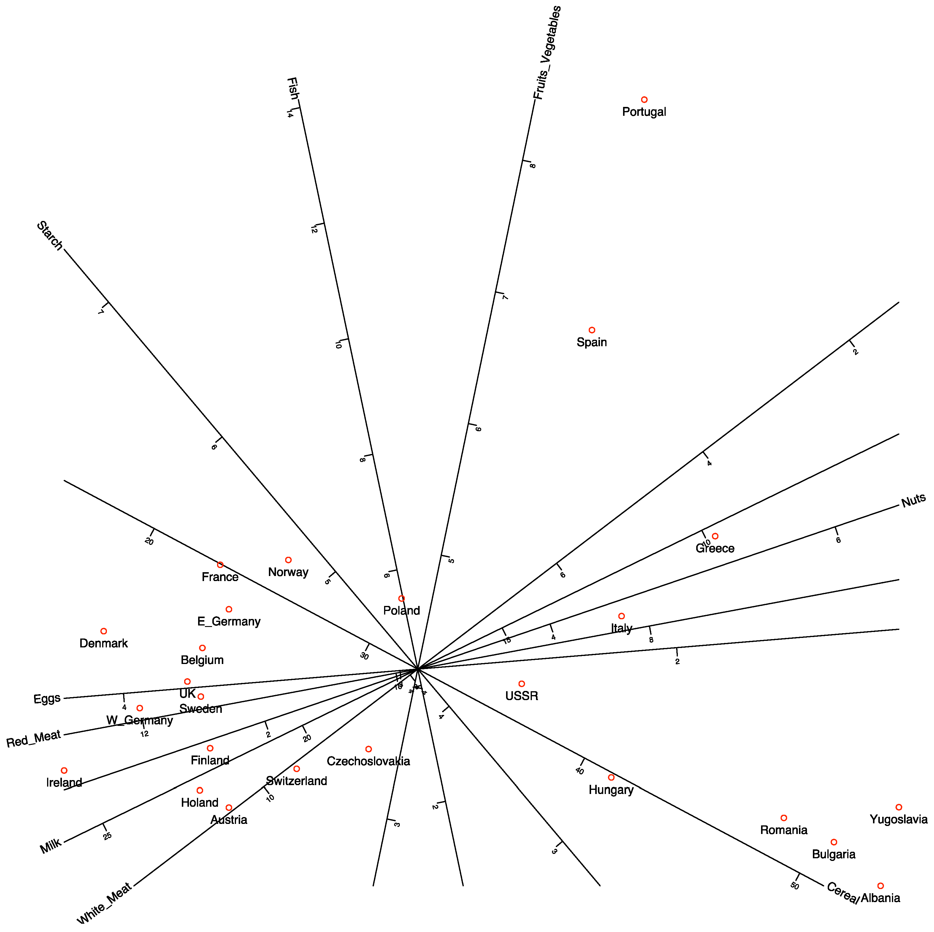
Therefore, the unit marker for the j-th variable is computed by dividing the coordinates of its corresponding marker by its squared length. Several points for specific values of $\mu$ can be labeled to obtain a reference scale. If the data are centered, then $b_{j0}=0$, and the labels can be calculated by adding the average to the value of $\mu$, i.e., $\mu +{\overline{x}}_j$. The resulting representation is shown in Figure 1. The data for this representation can be found in Weber [28] and were used to build a biplot by Gabriel [29].

Figure 1. Typical PCA biplot with scales for the variables.

The data contain the consumption of different types of proteins in various European countries. The aim is to detect groups of countries with similar behaviors and the variables responsible for them.

The biplot allows for the direct interpretation of the relationships between rows and columns, rather than the indirect relation through the principal components.

If $\widehat{\mathbf{X}}$ denotes the expected values of the biplot in the reduced dimension, $\widehat{\mathbf{X}}\approx {\mathbf{A}\mathbf{B}}^T$, the global goodness of fit is the amount of variability accounted for by the prediction, that is,

$${\rho }^2={\displaystyle \frac{\mathrm{tr}\left({\widehat{\mathbf{X}}}^T\widehat{\mathbf{X}}\right)}{\mathrm{tr}\left({\mathbf{X}}^T\mathbf{X}\right)}}.$$

(10)

Even for matrices in which we obtain a good global fit, there may be some columns whose information is not accounted for in the plot. The goodness of fit for each column is

$${\rho }_j^2={\displaystyle \frac{\mathrm{diag}\left({\widehat{\mathbf{X}}}^T\widehat{\mathbf{X}}\right)}{\mathrm{diag}\left({\mathbf{X}}^T\mathbf{X}\right)}},$$

(11)

where the division is performed element-wise. The quantity ${\rho }_j^2$ is also the $R^2$ of the regression of each column of $\mathbf{X}$ on $\mathbf{A}$, as in Equation (8). We refer to this quantity as the quality of representation of the variable. Gardner-Lubbe et al. [30] call this the predictiveness of the column. These measures are used to identify which variables are most related to the representation, or those whose information is preserved in the biplot. If two dimensions are not sufficient to account for the desired information, additional components can be used, and the quality measures can be recalculated by adapting Equations (10) and (11) to the desired number of dimensions.

2.2. Logistic Biplot for Binary Data

2.2.1. Formulation and Geometry of the Binary Logistic Biplot

Let $p_{ij}$$(i=1,\dots ,I;j=1,\dots ,J)$ be the observed probability, either 0 or 1, that an individual i possesses characteristic j, resulting in a binary data matrix ${\mathbf{P}}_{I\times J}$. The S-dimensional logistic principal components model (logistic biplot) is given by

$${\pi }_{ij}={\displaystyle \frac{e^{b_{j0}+{\sum }_k{b}_{jk}{a}_{ik}}}{1+e^{b_{j0}+{\sum }_k{b}_{jk}{a}_{ik}}}}={\displaystyle \frac{1}{1+e^{-\left(b_{j0}+{\sum }_k{b}_{jk}{a}_{ik}\right)}}},$$

(12)

or, on the logit scale,

$$\mathrm{logit}\left({\pi }_{ij}\right)=log\left({\displaystyle \frac{{\pi }_{ij}}{1-{\pi }_{ij}}}\right)=b_{j0}+\sum _{s=1}^S{b}_{js}{a}_{is}=b_{j0}+{\mathbf{a}}_i^T{\mathbf{b}}_j,$$

(13)

where ${\pi }_{ij}=\mathbb{E}\left(p_{ij}\right)$ denotes the expected probabilities that individual i possesses characteristic j, and $a_{is}$ and $b_{js}$$(i=1,\dots ,I;j=1,\dots ,J;s=1,\dots ,S)$ are the model parameters used as row and column markers, respectively. The model is a generalized bilinear model with the logit function serving as the link.

In matrix form:

$$\mathrm{logit}\left(\mathbf{\Pi }\right)={\mathbf{1}}_I{\mathbf{b}}_0^T+\mathbf{A}{\mathbf{B}}^T,$$

(14)

where $\mathbf{\Pi }$ is the matrix of expected probabilities, ${\mathbf{1}}_I$ is a vector of ones, and ${\mathbf{b}}_0=(b_{10},\dots ,b_{J0})$ is the vector of intercepts. These intercepts are included because it is not possible to center the data matrix in the same way as in linear biplots.

The points predicting different probabilities lie on parallel straight lines in the biplot. This means that predictions in the logistic biplot are made in the same way as in linear biplots—i.e., by projecting a row marker ${\mathbf{a}}_i=(a_{i1},a_{i2})$ onto a column marker ${\mathbf{b}}_j=(b_{j1},b_{j2})$ (see [7] or [8]).

The calculations required to obtain the scale markers are straightforward. To find the marker for a fixed probability $\pi$, we look for the point $(x,y)$ that predicts $\pi$ and lies along the direction of ${\mathbf{b}}_j$, i.e., on the line connecting the origin $(0,0)$ and the point $(b_{j1},b_{j2})$. That is,

$$y={\displaystyle \frac{b_{j2}}{b_{j1}}}x,$$

and

$$\mathrm{logit}\left(\pi \right)=b_{j0}+b_{j1}x+b_{j2}y.$$

Solving for x and y, we obtain

$$x={\displaystyle \frac{(\mathrm{logit}\left(\pi \right)-b_{j0})b_{j1}}{b_{j1}^2+b_{j2}^2}}\mathrm{and}y={\displaystyle \frac{(\mathrm{logit}\left(\pi \right)-b_{j0})b_{j2}}{b_{j1}^2+b_{j2}^2}}.$$

Several points corresponding to specific values of $\pi$ can be labeled to obtain a reference scale. From a practical point of view, the most informative value is $\pi =0.5$, because the line passing through that point and perpendicular to the direction divides the representation into two regions: one predicting presence and the other absence. Plotting that point together with an arrow indicating the direction of increasing probabilities is sufficient for most practical applications.

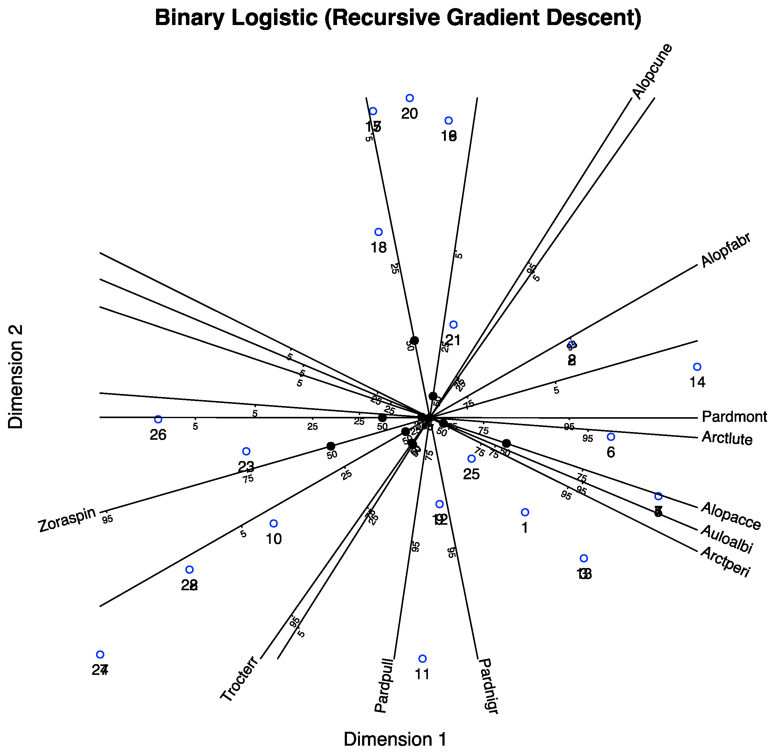
A typical representation of a binary logistic biplot is given in Figure 2.

Figure 2. Typical binary logistic biplot with probability scales for the variables.

2.2.2. Parameter Estimation

The model in Equation (12) is also a latent trait model, or Item Response Theory (IRT) model, in which the ordination axes are treated as latent variables that explain the associations among the observed variables. In this framework, it is assumed that individuals respond independently to variables, and that the variables are conditionally independent given the values of the latent traits.

Under these assumptions, the likelihood function is

$$\mathrm{Prob}(p_{ij}\mid {\mathbf{b}}_0,\mathbf{A},\mathbf{B})=\prod _{i=1}^I\prod _{j=1}^J{\pi }_{ij}^{p_{ij}}{(1-{\pi }_{ij})}^{1-p_{ij}}.$$

(15)

Taking the logarithm of the likelihood function yields

$$L=log\left(\mathrm{Prob}(p_{ij}\mid {\mathbf{b}}_0,\mathbf{A},\mathbf{B})\right)=\sum _{i=1}^I\sum _{j=1}^J\left[p_{ij}log\left({\pi }_{ij}\right)+(1-p_{ij})log(1-{\pi }_{ij})\right].$$

(16)

For fixed $\mathbf{A}$, Equation (16) can be separated into J components, one for each variable:

$$L=\sum _{j=1}^J{L}_j=\sum _{j=1}^J\left(\sum _{i=1}^I\left[p_{ij}log\left({\pi }_{ij}\right)+(1-p_{ij})log(1-{\pi }_{ij})\right]\right).$$

(17)

Maximizing each $L_j$ is equivalent to performing a standard logistic regression, using the j-th column of $\mathbf{X}$ as the response and the columns of $\mathbf{A}$ as predictors.

In the same way that the likelihood function can be separated into parts for each variable, it can also be partitioned into components for each row of the data matrix: $L={\sum }_{i=1}^I{L}_i$. The details of the procedure used to calculate the row or individual scores can be found in [7]. Binary logistic biplots computed in this manner are available in the package MULTBIPLOT [31].

This estimation procedure may be affected by the separation problem, which occurs when, in the reduced-dimensional subspace, there exists a hyperplane that completely separates presences from absences for any of the observed variables. In such cases, the maximum likelihood method does not converge.

Alternative estimation methods, such as Marginal Maximum Likelihood, can be found in [20], within the context of Item Response Theory (IRT).

Vicente-Gonzalez and Vicente-Villardon [32] employed gradient descent methods, where the cost function is defined as the negative log-likelihood:

$$L=\sum _{i=1}^I\sum _{j=1}^J\left[-p_{ij}log\left({\pi }_{ij}\right)-(1-p_{ij})log(1-{\pi }_{ij})\right].$$

(18)

Here, the function is interpreted as a cost to minimize, rather than a likelihood to maximize. The objective is to find the parameters $\mathbf{A}$, $\mathbf{B}$, and ${\mathbf{b}}_0$ that minimize the cost function.

Since there are no closed-form solutions for this optimization problem, an iterative algorithm is employed to generate a sequence of decreasing values of the cost function. We use the gradient descent method recursively, updating one component at a time while holding the others fixed. The updates for each parameter are as follows:

$$\begin{array}{cc}\hfill b_{j0}& \Leftarrow b_{j0}-\alpha {\displaystyle \frac{\partial L}{\partial b_{j0}}}=b_{j0}-\alpha \sum _{i=1}^I({\pi }_{ij}-p_{ij}),\hfill \end{array}$$

(19)

$$\begin{array}{cc}\hfill a_{is}& \Leftarrow a_{is}-\alpha {\displaystyle \frac{\partial L}{\partial a_{is}}}=a_{is}-\alpha \sum _{j=1}^J{b}_{js}({\pi }_{ij}-p_{ij}),\hfill \end{array}$$

(20)

$$\begin{array}{cc}\hfill b_{js}& \Leftarrow b_{js}-\alpha {\displaystyle \frac{\partial L}{\partial b_{js}}}=b_{js}-\alpha \sum _{i=1}^I{a}_{is}({\pi }_{ij}-p_{ij}),\hfill \end{array}$$

(21)

for some learning rate $\alpha$.

Or, in matrix form, we have

$$\begin{array}{cc}\hfill {\mathbf{b}}_0& \Leftarrow {\mathbf{b}}_0-\alpha {(\mathbf{\Pi }-\mathbf{P})}^T{\mathbf{1}}_I,\hfill \end{array}$$

(22)

$$\begin{array}{cc}\hfill {\mathbf{a}}_{\left(s\right)}& \Leftarrow {\mathbf{a}}_{\left(s\right)}-\alpha (\mathbf{\Pi }-\mathbf{P}){\mathbf{b}}_{\left(s\right)},\hfill \end{array}$$

(23)

$$\begin{array}{cc}\hfill {\mathbf{b}}_{\left(s\right)}& \Leftarrow {\mathbf{b}}_{\left(s\right)}-\alpha {(\mathbf{\Pi }-\mathbf{P})}^T{\mathbf{a}}_{\left(s\right)},\hfill \end{array}$$

(24)

where ${\mathbf{a}}_{\left(s\right)}=(a_{1s},\dots ,a_{Is})$ and ${\mathbf{b}}_{\left(s\right)}=(b_{1s},\dots ,b_{Js})$.

For large data matrices, it may be convenient to summarize the data in a matrix $\mathbf{P}$ containing unique response patterns and a vector $\mathbf{f}$ containing the frequency of each pattern. In this case, the gradient descent updates become

$$\begin{array}{cc}\hfill {\mathbf{b}}_0& \Leftarrow {\mathbf{b}}_0-\alpha {(\mathbf{\Pi }-\mathbf{P})}^T\mathbf{f},\hfill \end{array}$$

(25)

$$\begin{array}{cc}\hfill {\mathbf{a}}_{\left(s\right)}& \Leftarrow {\mathbf{a}}_{\left(s\right)}-\alpha (\mathbf{\Pi }-\mathbf{P}){\mathbf{b}}_{\left(s\right)},\hfill \end{array}$$

(26)

$$\begin{array}{cc}\hfill {\mathbf{b}}_{\left(s\right)}& \Leftarrow {\mathbf{b}}_{\left(s\right)}-\alpha {(\mathbf{\Pi }-\mathbf{P})}^T(\mathbf{f}\odot {\mathbf{a}}_{\left(s\right)}),\hfill \end{array}$$

(27)

where ⊙ denotes the Hadamard (element-wise) product.

We can organize the computations into an alternating algorithm that sequentially estimates the parameters for rows and columns, for each dimension s, while keeping fixed the parameters already obtained for the previous dimensions.

Before proceeding, the intercepts ${\mathbf{b}}_0=(b_{10},\dots ,b_{J0})$ must be estimated separately. This step is analogous to subtracting column means to center the data matrix in the continuous biplot framework.

The procedure is as follows:

In practice, the choice of the learning rate $\alpha$ can be avoided by using a pre-programmed optimization routine.

This algorithm is implemented in the package MultBiplotR [33], developed in the R language [34]. A direct extension of this algorithm is described in [14] and is implemented in the package BiplotML [35].

Algorithm 1 outlines the alternating optimization procedure for the binary logistic biplot. Our proposed ordinal algorithm, introduced in Section 3.3, builds on similar principles, with the necessary modifications to accommodate ordinal outcomes.

Algorithm 1 Algorithm to calculate the components for binary data

1: procedure P-Binary-Components($\mathbf{P},S$)   2:     Choose $\alpha$   3:     Init: ${\mathbf{b}}_0=random$   4:     repeat   5:         Update: ${\mathbf{b}}_0$ with Equation (22) or (25)   6:         Update: $\mathbf{\Pi }=\left({\pi }_{ij}\right)$ with Equation (12)   7:     until ${\mathbf{b}}_0$ do not change   8:     for $s=1\to S$ do   9:         Init: ${\mathbf{a}}_{\left(s\right)}\leftarrow random$ (or any other choice) 10:         repeat 11:            repeat 12:                Update: ${\mathbf{b}}_{\left(s\right)}$ with Equation (24) or (27) 13:                Update: $\mathbf{\Pi }=\left({\pi }_{ij}\right)$ with Equation (12) 14:            until ${\mathbf{b}}_{\left(s\right)}$ do not change 15:            repeat 16:                Update: ${\mathbf{a}}_{\left(s\right)}$ with Equation (23) or (26) 17:                Update: $\mathbf{\Pi }=\left({\pi }_{ij}\right)$ with Equation (12) 18:            until ${\mathbf{a}}_{\left(s\right)}$ do not change 19:            $L\leftarrow (-1){\mathbf{1}}_I^T((\mathbf{P}\odot \mathbf{\Pi })+((1-\mathbf{P})\odot (1-\mathbf{\Pi }))){\mathbf{1}}_J$ 20:         until L does not change     return ${\mathbf{b}}_0$, $\mathbf{B}=\left[{\mathbf{b}}_{\left(1\right)},\dots ,{\mathbf{b}}_{\left(S\right)}\right]$, $\mathbf{A}=\left[{\mathbf{a}}_{\left(1\right)},\dots ,{\mathbf{a}}_{\left(S\right)}\right]$

2.3. Logistic Biplot for Nominal Data

Let ${\mathbf{X}}_{I\times J}$ be a data matrix containing the values of J nominal variables, each with $K_j$$(j=1,\dots ,J)$ categories, for I individuals. Let ${\mathbf{P}}_{I\times L}$ be the corresponding indicator matrix, with $L={\sum }_j{K}_j$ columns. The last (or the first) category of each variable will be used as a baseline.

Let ${\pi }_{ij\left(k\right)}$ denote the expected probability that individual i belongs to category k of variable j. A multinomial logistic latent trait model with S latent traits states that the probabilities are given by

$${\pi }_{ij\left(k\right)}={\displaystyle \frac{e^{b_{j\left(k\right)0}+{\displaystyle \sum _{s=1}^S}{b}_{j\left(k\right)s}{a}_{is}}}{{\displaystyle \sum _{l=1}^{K_j}}{e}^{b_{j\left(l\right)0}+{\displaystyle \sum _{s=1}^S}{b}_{j\left(l\right)s}{a}_{is}}}},(k=1,\dots ,K_j).$$

(28)

To make the model identifiable, the parameters for the baseline category (e.g., the last one) are constrained to zero, i.e., $b_{j\left(K_j\right)0}=b_{j\left(K_j\right)s}=0$ for all $j=1,\dots ,J$ and $s=1,\dots ,S$. With this restriction, the model becomes

$${\pi }_{ij\left(k\right)}={\displaystyle \frac{e^{b_{j\left(k\right)0}+{\displaystyle \sum _{s=1}^S}{b}_{j\left(k\right)s}{a}_{is}}}{1+{\displaystyle \sum _{l=1}^{K_j-1}}{e}^{b_{j\left(l\right)0}+{\displaystyle \sum _{s=1}^S}{b}_{j\left(l\right)s}{a}_{is}}}},(k=1,\dots ,K_j-1).$$

(29)

With this constraint, the log-odds of each response (relative to the baseline category) follow a linear model:

$$log\left({\displaystyle \frac{{\pi }_{ij\left(k\right)}}{{\pi }_{ij\left(K_j\right)}}}\right)=b_{j\left(k\right)0}+\sum _{s=1}^S{b}_{j\left(k\right)s}{a}_{is}=b_{j\left(k\right)0}+{\mathbf{a}}_i^T{\mathbf{b}}_{j\left(k\right)},$$

where $a_{is}$ and $b_{j\left(k\right)s}$ are the model parameters, with $i=1,\dots ,I$; $j=1,\dots ,J$; $k=1,\dots ,K_j-1$; and $s=1,\dots ,S$.

In matrix form:

$$\mathbf{O}={\mathbf{1}}_I{\mathbf{b}}_0^T+\mathbf{A}{\mathbf{B}}^T,$$

(30)

where ${\mathbf{O}}_{I\times (L-J)}$ is the matrix containing the expected log-odds. This defines a biplot for the log-odds. Although this representation may be useful, it is often more interpretable in terms of predicted probabilities and categorical outcomes.

This representation is referred to as the nominal logistic biplot, and it is related to latent nominal models in the same way that classical linear biplots are related to factor analysis or principal component analysis, and binary logistic biplots are related to Item Response Theory or latent trait analysis for binary data.

In this case, the points predicting different probabilities are no longer located on parallel straight lines. This means that predictions in the nominal logistic biplot are not made in the same way as in linear biplots; instead, the response surfaces define prediction regions for each category, as illustrated in [15]. The nominal logistic biplot is described here in less detail, as its geometry is less directly related to our proposal than to that of the linear or binary logistic biplot.

3. Logistic Biplot for Ordinal Data

3.1. Formulation and Geometry of the Ordinal Logistic Biplot

Let ${\mathbf{X}}_{I\times J}$ be a data matrix containing the measurements of I individuals on J ordinal variables, each with $K_j$ ordered categories $(j=1,\dots ,J)$. Let ${\mathbf{P}}_{I\times L}$ be the corresponding indicator matrix, with $L={\sum }_j{K}_j$ columns.

For each ordinal variable $X_j$, let ${\mathbf{P}}_j$ be an indicator matrix of size $I\times K_j$, containing binary indicators for each category. Then the full indicator matrix is defined as $\mathbf{P}=\left({\mathbf{P}}_1,\dots ,{\mathbf{P}}_J\right)$. Each row of ${\mathbf{P}}_j$ sums to 1, and each row of $\mathbf{P}$ sums to J. Therefore, $\mathbf{P}$ can be interpreted as a matrix of observed probabilities for each category of each variable.

We also define the cumulative observed probabilities as

$$p_{ij\left(k\right)}^{*}=\left\{\begin{array}{cc}1\hfill & \mathrm{if}{x}_{ij}\le k,\hfill \\ 0\hfill & \mathrm{otherwise},\hfill \end{array}\right.\mathrm{for}k=1,\dots ,K_j-1,$$

that is, as binary indicators of the cumulative categories. Note that $p_{ij\left(K_j\right)}^{*}=1$ for all i, so the last category can be omitted without loss of information.

We organize the cumulative indicators for variable $X_j$ into a matrix ${\mathbf{P}}_j^{*}=\left(p_{ij\left(k\right)}^{*}\right)$ of size $I\times (K_j-1)$. Then the full cumulative indicator matrix is defined as

$${\mathbf{P}}^{*}=\left({\mathbf{P}}_1^{*},\dots ,{\mathbf{P}}_J^{*}\right),$$

which has dimensions $I\times (L-J)$ and contains the observed cumulative probabilities for all ordinal variables.

Let ${\pi }_{ij\left(k\right)}^{*}=P(x_{ij}\le k)$ be the (expected) cumulative probability that individual i has a value less than or equal to k on the j-th ordinal variable, and let ${\pi }_{ij\left(k\right)}=P(x_{ij}=k)$ be the (expected) probability that individual i takes the k-th value on the j-th ordinal variable. Then ${\pi }_{ij\left(K_j\right)}^{*}=P(x_{ij}\le K_j)=1$, and ${\pi }_{ij\left(k\right)}={\pi }_{ij\left(k\right)}^{*}-{\pi }_{ij(k-1)}^{*}$ (with ${\pi }_{ij\left(0\right)}^{*}=0$).

A multidimensional (i.e., S-dimensional) logistic latent trait model for the cumulative probabilities can be written as follows for $1\le k\le K_j-1$:

$${\pi }_{ij\left(k\right)}^{*}={\displaystyle \frac{1}{1+e^{-\left(d_{j\left(k\right)}+{\sum }_{s=1}^S{a}_{is}{b}_{js}\right)}}}={\displaystyle \frac{1}{1+e^{-\left(d_{j\left(k\right)}+{\mathbf{a}}_i^T{\mathbf{b}}_j\right)}}}$$

(31)

where ${\mathbf{a}}_i={(a_{i1},\dots ,a_{iS})}^{\prime }$ is the vector of latent trait scores for the i-th individual, and $d_{j\left(k\right)}$ and ${\mathbf{b}}_j={(b_{j1},\dots ,b_{jS})}^{\prime }$ are the parameters for each item or variable.

Note that we have defined a set of binary logistic models, one for each category, each with a different intercept but a common set of slopes. In the context of Item Response Theory (IRT), this is known as the graded response model or Samejima’s model [36]. The main difference from IRT models is that we do not impose the restriction that the probability of obtaining a higher category must increase along the dimensions. Our variables are not necessarily items from a test, but the models are formally the same in both cases.

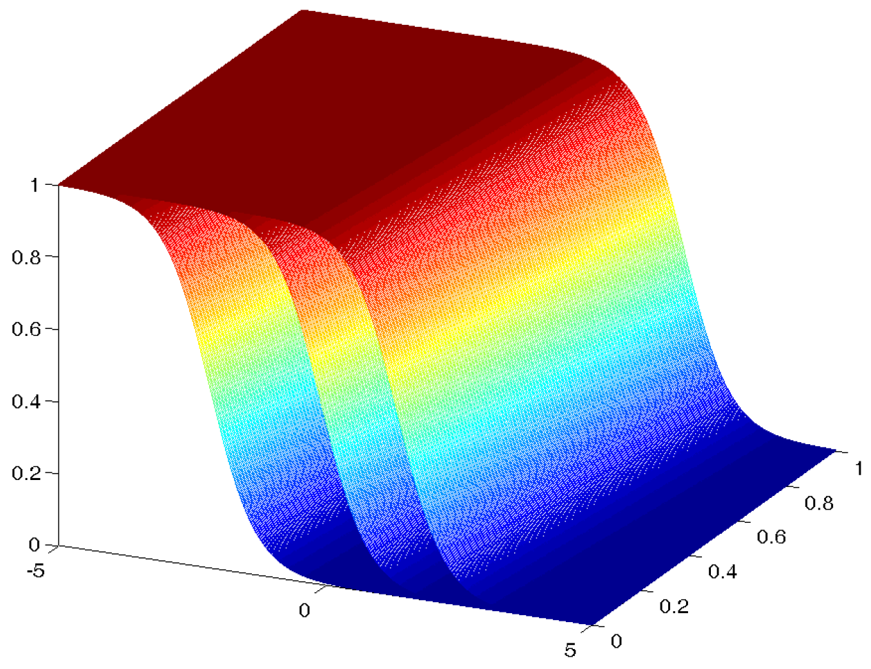
In the unidimensional case, the model corresponds to one with a unique discrimination parameter $b_j$ for all categories and different thresholds, boundaries, difficulties, or location parameters $d_{j\left(k\right)}$. The two-dimensional cumulative model is shown in Figure 3.

Figure 3. Cumulative response curves for a two-dimensional latent trait and a variable with four categories.

The ${\mathbf{a}}_i$ scores can be represented in a scatter diagram and used to identify similarities and differences among individuals or to search for clusters with homogeneous characteristics; that is, the representation resembles that obtained from any multidimensional scaling method.

In the following, we will show that the ${\mathbf{b}}_j$ parameters can also be represented on the graph as directions in the score space that best predict probabilities and help identify the variables or items responsible for differences among individuals.

On the logit scale, the model is given by

$$\mathrm{logit}\left({\pi }_{ij\left(k\right)}^{*}\right)=d_{j\left(k\right)}+\sum _{s=1}^S{a}_{is}{b}_{js}=d_{j\left(k\right)}+{\mathbf{a}}_i^T{\mathbf{b}}_j,k=1,\dots ,K_j-1$$

(32)

This defines a binary logistic biplot for the cumulative categories.

In matrix form:

$$\mathrm{logit}\left({\mathbf{\Pi }}^{*}\right)=\mathbf{1}{\mathbf{d}}^{\prime }+{\mathbf{AB}}^{\prime }$$

(33)

where ${\mathbf{\Pi }}^{*}=({\mathrm{\Pi }}_1^{*},\dots ,{\mathrm{\Pi }}_J^{*})$ is the $I\times (L-J)$ matrix of expected cumulative probabilities, ${\mathbf{1}}_I$ is a vector of ones, and $\mathbf{d}={({\mathbf{d}}_1^T,\dots ,{\mathbf{d}}_J^T)}^T$, with ${\mathbf{d}}_j^T=(d_{j\left(1\right)},\dots ,d_{j(K_j-1)})$, is the vector containing the thresholds.

$\mathbf{A}={({\mathbf{a}}_1^T,\dots ,{\mathbf{a}}_I^T)}^{\prime }$, with ${\mathbf{a}}_i^T=(a_{i1},\dots ,a_{iS})$, is the $I\times S$ matrix of individual scores, and $\mathbf{B}={({\mathbf{B}}_1^T,\dots ,{\mathbf{B}}_J^T)}^{\prime }$, where ${\mathbf{B}}_j={\mathbf{1}}_{K_j-1}\otimes {\mathbf{b}}_j^T$ and ${\mathbf{b}}_j^T=(b_{j1},\dots ,b_{jS})$, is the $(L-J)\times S$ matrix containing the slopes for all variables.

This expression defines a biplot for the odds, which will be referred to as the ordinal logistic biplot. Each equation of the cumulative biplot shares the geometry described in the binary case [7]; moreover, all curves share the same direction when projected onto the biplot.

The set of parameters $\left\{d_{j\left(k\right)}\right\}$ provides a different threshold for each cumulative category. The second part of Equation (32) does not depend on the particular category, meaning that all the $K_j-1$ curves share the same slopes.

In the following paragraphs, we derive the geometry for the general case and present an algorithm to perform the necessary calculations.

The expected probability of individual i responding in category k to item j (with $k=1,\dots ,K_j$), denoted by ${\pi }_{ij\left(k\right)}=P(x_{ij}=k)$, must be obtained by subtracting cumulative probabilities:

$${\pi }_{ij\left(k\right)}={\pi }_{ij\left(k\right)}^{*}-{\pi }_{ij(k-1)}^{*}$$

Then, using the expressions from Equation (31),

$$\begin{array}{cc}\hfill {\pi }_{ij\left(1\right)}& =P(x_{ij}=1)={\displaystyle \frac{1}{1+e^{-(d_{j\left(1\right)}+{\mathbf{a}}_i^T{\mathbf{b}}_j)}}}\hfill \\ \hfill {\pi }_{ij\left(k\right)}& =P(x_{ij}=k)=P(x_{ij}\le k)-P(x_{ij}\le k-1)\hfill \\ \hfill & ={\displaystyle \frac{1}{1+e^{-(d_{j\left(k\right)}+{\mathbf{a}}_i^T{\mathbf{b}}_j)}}}-{\displaystyle \frac{1}{1+e^{-(d_{j(k-1)}+{\mathbf{a}}_i^T{\mathbf{b}}_j)}}}\hfill \\ \hfill & ={\displaystyle \frac{e^{-{\mathbf{a}}_i^T{\mathbf{b}}_j}(e^{-d_{j(k-1)}}-e^{-d_{j\left(k\right)}})}{(1+e^{-(d_{j\left(k\right)}+{\mathbf{a}}_i^T{\mathbf{b}}_j)})(1+e^{-(d_{j(k-1)}+{\mathbf{a}}_i^T{\mathbf{b}}_j)})}},1<k<K_j\hfill \\ \hfill {\pi }_{ij\left(K_j\right)}& =P(x_{ij}=K_j)=1-{\displaystyle \frac{1}{1+e^{-(d_{j(K_j-1)}+{\mathbf{a}}_i^T{\mathbf{b}}_j)}}}\hfill \end{array}$$

(34)

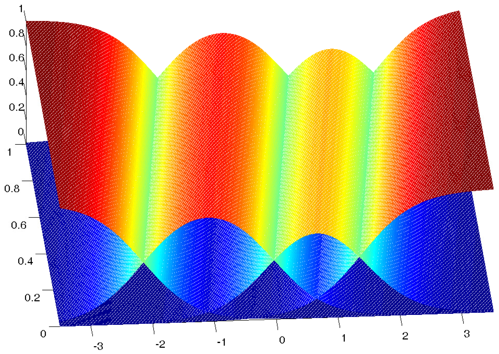
If the row scores were known, obtaining the parameters of the model in Equation (34) would be equivalent to fitting a proportional odds model, using each item as a response and the row scores as regressors. The response surfaces for such a model are shown in Figure 4.

Figure 4. Response curves for an ordinal variable with four ordered categories.

Although the response surfaces are no longer sigmoidal, the level curves remain straight lines. Therefore, the set of points in the representation (generated by the columns of $\mathbf{A}$) that predict a particular value for the probability of a category lie along a straight line. Furthermore, different probabilities for all the categories of a particular variable or item lie along parallel straight lines. A line perpendicular to all of these can be used as a biplot axis in the sense of Gower and Hand [2]; this is the direction that best predicts the probabilities of all the categories. That is, by projecting any individual point onto this direction, one obtains an optimal prediction of the category probabilities.

As all categories share the same biplot direction, it becomes impractical to display a different graded scale for each. Instead, we represent only the line segments along which the probability of a particular category is higher than the probabilities of the others. Except in pathological cases, this results in as many segments as there are categories ($K_j$), separated by $K_j-1$ points, where the probabilities of two contiguous categories are equal.

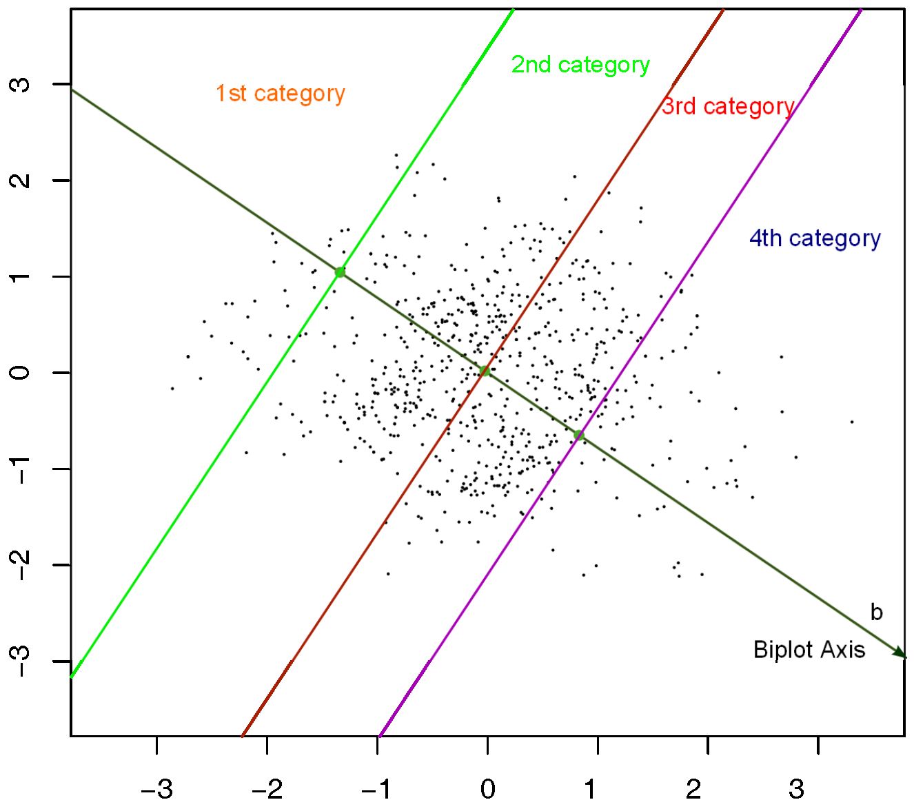
See Figure 5, where we illustrate the parallel lines representing the points that predict equal probabilities for two contiguous categories, and a line—perpendicular to all—that serves as the biplot axis. The three parallel lines divide the space spanned by the columns of $\mathbf{A}$ into four regions, each predicting a specific category of the variable. For the biplot representation, we do not require the entire set of lines, but only the axis and the points where it intersects the boundaries between prediction regions.

Figure 5. Prediction regions determined by three parallel straight lines for an ordinal variable with four categories.

3.2. Obtaining the Biplot Representation

So, if $(x,y)$ denotes one of these intersection points, it must lie on the biplot direction. That is,

$$y={\displaystyle \frac{b_{j2}}{b_{j1}}}x$$

(35)

and the probabilities of two, possibly contiguous categories (for example, l and m) at this point must be equal:

$${\pi }_{j\left(l\right)}={\pi }_{j\left(m\right)}\left({\pi }_{j\left(l\right)}^{*}-{\pi }_{j(l-1)}^{*}={\pi }_{j\left(m\right)}^{*}-{\pi }_{j(m-1)}^{*}\right).$$

(36)

We have omitted the index i because the probabilities refer to a general point rather than a specific individual. Using the condition in Equation (35), we can rewrite the cumulative probabilities (or their logits) as

$$\mathrm{logit}\left({\pi }_{j\left(k\right)}^{*}\right)=d_{j\left(k\right)}+x{b}_{j1}+y{b}_{j2}=d_{j\left(k\right)}+z$$

(37)

with

$$z=x\left({\displaystyle \frac{b_{j1}^2+b_{j2}^2}{b_{j1}}}\right)$$

(38)

By varying the value of z, we can compute the probabilities of each category along the biplot axis. Thus, finding the point $(x,y)$ is equivalent to finding the values of z for which Equation (36) holds. Once those values are found, the original coordinates can be recovered by solving for x in Equation (38), and then computing y from Equation (35).

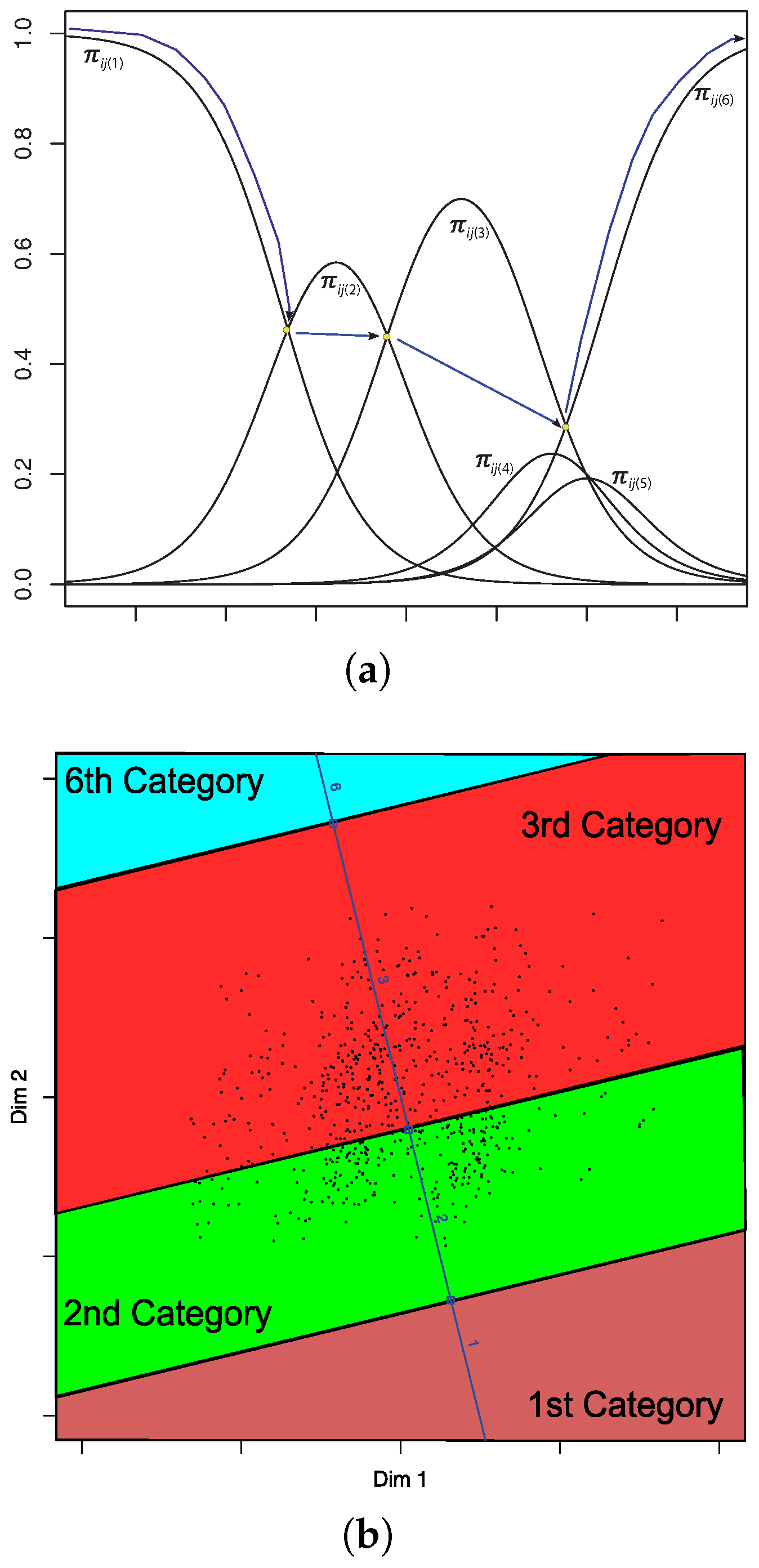
There are some pathological cases in which the probability of one or more categories is never higher than the probability of the others. In such cases, we say that the category is “hidden” or “never predicted,” and the number of separating points will be fewer than $K_j-1$. These pathological cases must be taken into account when calculating the intersection points. See Figure 6.

Figure 6. Probability curves for a variable with 6 categories, of which 2 (4 and 5) are hidden or never predicted. (a) Projection of the response curves onto a plane perpendicular to the biplot axis. (b) Final representation without the hidden categories.

The existence of abnormal cases means that not only contiguous but all pairs of categories may have to be compared. Many such comparisons are possible because the corresponding equations differ for each case:

• 1–2;
• 1–$l(l<K_j)$;
• 1–$K_j$;
• l–$K_j(l>1)$;
• l–$(l+1)(l>1)$;
• l–$j(j>l+1,l>1)$;
• $(K_j-1)$–$K_j$.

For example, in case (3), 1–$K_j$, it is simple to deduce that

$$z={\displaystyle \frac{-\left(d_{j(K_j-1)}+d_{j\left(1\right)}\right)}{2}}.$$

Cases (1), (3), (5), and (7) are straightforward. In the other three combinations, we must solve a quadratic equation to obtain the intersection points.

For example, in case (2)—the first involving the l-th category—we must solve ${\pi }_{j\left(1\right)}={\pi }_{j\left(l\right)}$, that is,

$${\displaystyle \frac{1}{1+e^{-(d_{j\left(1\right)}+z)}}}={\displaystyle \frac{e^{-z}\left(e^{-d_{j(l-1)}}-e^{-d_{j\left(l\right)}}\right)}{\left(1+e^{-(d_{j\left(l\right)}+z)}\right)\left(1+e^{-(d_{j(l-1)}+z)}\right)}}.$$

Taking $w=e^{-z}$, we obtain the quadratic equation

$$\alpha w^2-\beta w-1=0,$$

where

$$\alpha =e^{-(d_{j\left(1\right)}+d_{j(l-1)})}-e^{-(d_{j\left(1\right)}+d_{j\left(l\right)})}-e^{-(d_{j(l-1)}+d_{j\left(l\right)})},\beta =2e^{-d_{j\left(1\right)}}.$$

If both roots of the equation are negative, the curves do not intersect. If there is a positive root, we can compute the intersection point by solving for w and then reversing the transformation to obtain $(x,y)$.

In a similar way, the intersection points for cases (4), i–$K_j$ $(i>1)$, and (6), i–j with $j>i+1$, can be calculated.

• Calculate the biplot axis using the equation

  $$y={\displaystyle \frac{b_{j2}}{b_{j1}}}x.$$
• Calculate the intersection points z, and then $(x,y)$, of the biplot axis with the parallel lines that serve as boundaries of the prediction regions for each pair of categories, in the following order:

  $$\begin{array}{cc}\hfill {\pi }_{j\left(1\right)}& ={\pi }_{j\left(2\right)}\hfill \\ \hfill {\pi }_{j(l-1)}& ={\pi }_{j\left(l\right)}\mathrm{for}1<l<K_j-1\hfill \\ \hfill {\pi }_{j(K_j-1)}& ={\pi }_{j\left(K_j\right)}\hfill \end{array}$$
• If the values of z are ordered, there are no hidden categories, and the calculations are complete.
• If the z values are not ordered, proceed as follows:

  (a)

  Calculate the z values for all pairs of curves and evaluate the probabilities for the two categories involved.

  (b)

  Compare each category with the next. The next category to represent is the one with the highest probability at the intersection.

  (c)

  If the next category is $K_j$, the process is complete. If not, return to the previous step, starting with the new category.

A simpler numerical method can be developed to avoid the explicit solution of equations:

• Evaluate the predicted category for a sequence of z values, for example, from $-6$ to 6 using small steps (e.g., 0.01). The precision of the algorithm can be adjusted via the step size.
• Identify the z values at which the predicted category changes.
• Compute the mean of each pair of consecutive z values where a change occurs, and then derive the corresponding $(x,y)$ values. These points are the desired intersection points.

Categories with zero frequencies in the prediction sequence are considered “hidden” or “never predicted.”

3.3. Parameter Estimation Based on an Alternating Gradient Descent Algorithm on the Cumulative Probabilities

The alternating algorithm described in [7] can be easily extended by replacing binary logistic regressions with ordinal logistic regressions. However, a limitation of this approach is that the individual parameters cannot be estimated when an individual has responses of only 0 or 1 across all variables in the binary case, or when all responses fall into the baseline category in the ordinal case.

Additional issues arise when perfect probability predictions occur, leading to a situation of perfect separation between some categories. This procedure is similar to the joint maximum likelihood estimation used in Item Response Theory (IRT) models. An algorithm for cumulative probabilities has been developed in [26].

We propose an alternative algorithm based on an alternating gradient descent procedure and the biplot representation described earlier.

We use cumulative probabilities in combination with a recursive procedure, similar to that used for binary data, based on gradient descent methods. The cost function based on cumulative probabilities is given by

$$L=-\sum _{i=1}^I\sum _{j=1}^J\sum _{k=1}^{K_j}{p}_{ij\left(k\right)}^{*}log\left({\pi }_{ij\left(k\right)}^{*}\right),$$

(39)

where the expected cumulative probabilities are defined as

$${\pi }_{ij\left(k\right)}^{*}={\displaystyle \frac{1}{1+exp\left(-\left(d_{j\left(k\right)}+{\sum }_{s=1}^S{a}_{is}{b}_{js}\right)\right)}}={\displaystyle \frac{1}{1+exp\left(-\left(d_{j\left(k\right)}+{\mathbf{a}}_i^T{\mathbf{b}}_j\right)\right)}}.$$

(40)

We employ a recursive procedure similar to that used in the binary case, where the thresholds $d_{jk}$ are estimated first. Once these are fixed, the parameters for the latent dimensions are estimated one at a time. This approach is analogous to subtracting the mean in the case of continuous data.

As noted by a reviewer, the location parameters $d_{jk}$ are closely related to quantile regression [37], as they correspond to the quantiles of a standard normal distribution defined by the category frequencies of the variable. However, rather than employing a quantile-based method, we have used a gradient-based approach to estimate these constants, in order to maintain a compact and unified algorithmic structure.

The gradients for the binary case generalize naturally to the ordinal case by using cumulative probabilities. The parameter updates are then given by

$$\begin{array}{cc}\hfill d_{j\left(k\right)}& \leftarrow d_{j\left(k\right)}-\alpha {\displaystyle \frac{\partial L}{\partial d_{j\left(k\right)}}}=d_{j\left(k\right)}-\alpha \sum _{i=1}^I\left({\pi }_{ij\left(k\right)}^{*}-p_{ij\left(k\right)}^{*}\right),\hfill \end{array}$$

(41)

$$\begin{array}{cc}\hfill a_{is}& \leftarrow a_{is}-\alpha {\displaystyle \frac{\partial L}{\partial a_{is}}}=a_{is}-\alpha \sum _{j=1}^J{b}_{js}\sum _{k=1}^{K_j}\left({\pi }_{ij\left(k\right)}^{*}-p_{ij\left(k\right)}^{*}\right),\hfill \end{array}$$

(42)

$$\begin{array}{cc}\hfill b_{js}& \leftarrow b_{js}-\alpha {\displaystyle \frac{\partial L}{\partial b_{js}}}=b_{js}-\alpha \sum _{i=1}^I{a}_{is}\sum _{k=1}^{K_j}\left({\pi }_{ij\left(k\right)}^{*}-p_{ij\left(k\right)}^{*}\right).\hfill \end{array}$$

(43)

Let ${\mathbf{a}}_s={(a_{1s},\dots ,a_{Is})}^T$ and ${\mathbf{b}}_s={(b_{1s},\dots ,b_{Js})}^T$ be the vectors containing the row and column parameters for dimension s. Let $\mathbf{Z}$ be an $(L-J)\times J$ indicator matrix in which the j-th column takes the value 1 for the rows corresponding to the categories of the j-th variable, and 0 elsewhere. Then, the columns of the matrix

$$\mathbf{R}=({\mathbf{\Pi }}^{*}-{\mathbf{P}}^{*})\mathbf{Z}$$

(44)

contain $r_{ij}={\sum }_{k=1}^{K_j}({\pi }_{ij\left(k\right)}^{*}-p_{ij\left(k\right)}^{*})$ for each variable j.

The updates can then be written in matrix form as

$$\begin{array}{cc}\hfill \mathbf{d}& \leftarrow \mathbf{d}-\alpha {({\mathbf{\Pi }}^{*}-{\mathbf{P}}^{*})}^T{\mathbf{1}}_I,\hfill \end{array}$$

(45)

$$\begin{array}{cc}\hfill {\mathbf{a}}_s& \leftarrow {\mathbf{a}}_s-\alpha \mathbf{R}{\mathbf{b}}_s,\hfill \end{array}$$

(46)

$$\begin{array}{cc}\hfill {\mathbf{b}}_s& \leftarrow {\mathbf{b}}_s-\alpha {\mathbf{R}}^T{\mathbf{a}}_s.\hfill \end{array}$$

(47)

For large data matrices, it may be convenient to summarize the data into a matrix $\mathbf{X}$ (and the corresponding matrix of expected probabilities $\mathbf{P}$) that contains the unique response patterns, along with a vector $\mathbf{f}$ representing the frequency of each pattern. In this case, the gradient descent updates can be written as

$$\begin{array}{cc}\hfill \mathbf{d}& \leftarrow \mathbf{d}-\alpha {({\mathbf{\Pi }}^{*}-{\mathbf{P}}^{*})}^T\mathbf{f},\hfill \end{array}$$

(48)

$$\begin{array}{cc}\hfill {\mathbf{a}}_s& \leftarrow {\mathbf{a}}_s-\alpha \mathbf{R}{\mathbf{b}}_s,\hfill \end{array}$$

(49)

$$\begin{array}{cc}\hfill {\mathbf{b}}_s& \leftarrow {\mathbf{b}}_s-\alpha {\mathbf{R}}^T(\mathbf{f}\odot {\mathbf{a}}_s),\hfill \end{array}$$

(50)

where ⊙ denotes the Hadamard (element-wise) product.

We organize the optimization as an alternating algorithm (Algorithm 2), which iteratively updates the row and column parameters for each dimension s, fixing the parameters already estimated for the previous dimensions. Prior to this, the constants $d_{j\left(k\right)}$ must be estimated independently.

This algorithm produces decreasing values of the cost function and will eventually converge, at least to a local minimum. A useful strategy is to initialize the algorithm from multiple starting points and select the solution corresponding to the lowest achieved cost.

In practice, the choice of $\alpha$ can be avoided by using a pre-programmed optimization routine. In R, we have used the conjugated gradient method in the optimr routine, although other alternatives could be used. It is also convenient to standardize the row parameters for identification of the model. Here we have standard coordinates for the rows in the biplot, and the emphasis is on the variables, like in the classical Column Metric Preserving (CMP) or GH biplot.

We can observe that updating the column parameters is essentially fitting an ordinal logistic regression that can be affected by the problem of separation or perfect predictions. To avoid separation, the usual solution is to use a penalized likelihood [38]. This adds a penalty term to the likelihood function that encourages the coefficients to be smaller. In our case, we will use the Ridge penalty [39]:

$$L=-\sum _{i=1}^I\sum _{j=1}^J\sum _{k=1}^{K_j}{p}_{ij\left(k\right)}^{*}log\left({\pi }_{ij\left(k\right)}^{*}\right)+\lambda \sum _{j=1}^J\sum _{s=1}^S{b}_{js}^2.$$

(51)

Gradient adaptation for the penalized cost function is automatic. We may try several values of penalization $lambda$ to select the adequate value. In the application, we have used a penalization of $lambda=0.2$.

This algorithm will be implemented in the new version of package MultBiplotR ([33]) developed for the R language ([34]). The algorithm implementation in R is also available from the authors.

Algorithm 2 Algorithm to calculate components for ordinal data

1: procedure P-Ordinal-Components($\mathbf{P},S$)   2:     Choose the learning rate $\alpha$ (optional if using an optimization routine)   3:     Set tolerance and maximum number of iterations (e.g., ${10}^{-5}$ and 500)   4:     Initialize thresholds: $\mathbf{d}\leftarrow \mathrm{random}$                          ▹ Step 1: Estimate thresholds $\mathbf{d}$   5:     repeat   6:         Update thresholds: $\mathbf{d}\leftarrow \mathbf{d}-\alpha ·\mathrm{Gradient}$ (Equation (45))   7:         Update cumulative probabilities: ${\mathbf{\Pi }}^{*}\leftarrow {\pi }_{ij\left(k\right)}^{*}$ using Equation (40)   8:     until Convergence of $\mathbf{d}$ (change below tolerance)                       ▹ Step 2: Estimate latent dimensions   9:     for $s=1$ to S do 10:         Initialize individual scores: ${\mathbf{a}}_{\left(s\right)}\leftarrow \mathrm{random}$ 11:         Set $\mathrm{Iterations}\leftarrow 0$ 12:         repeat 13:            $\mathrm{Iterations}\leftarrow \mathrm{Iterations}+1$                          ▹ Update column parameters 14:            $\mathrm{ColIterations}\leftarrow 0$ 15:            repeat 16:                $\mathrm{ColIterations}\leftarrow \mathrm{ColIterations}+1$ 17:                Update ${\mathbf{b}}_{\left(s\right)}$ using Equation (46) 18:                Update cumulative probabilities: ${\mathbf{\Pi }}^{*}\leftarrow {\pi }_{ij\left(k\right)}^{*}$ using Equation (40) 19:            until Convergence of ${\mathbf{b}}_{\left(s\right)}$ or max ColIterations reached                             ▹ Update row parameters 20:            $\mathrm{RowIterations}\leftarrow 0$ 21:            repeat 22:                $\mathrm{RowIterations}\leftarrow \mathrm{RowIterations}+1$ 23:                Update ${\mathbf{a}}_{\left(s\right)}$ using Equation (47) 24:                Optionally standardize ${\mathbf{a}}_{\left(s\right)}$ (for identifiability) 25:                Update cumulative probabilities: ${\mathbf{\Pi }}^{*}\leftarrow {\pi }_{ij\left(k\right)}^{*}$ using Equation (40) 26:            until Convergence of ${\mathbf{a}}_{\left(s\right)}$ or max RowIterations reached 27:            Compute cost: $$L\leftarrow -{\mathbf{1}}_I^T\left(\mathbf{P}\odot log\left(\mathbf{\Pi }\right)+(1-\mathbf{P})\odot log(1-\mathbf{\Pi })\right){\mathbf{1}}_J$$ 28:         until Convergence of L or maximum Iterations reached 29:     return thresholds $\mathbf{d}$, loadings $\mathbf{B}=[{\mathbf{b}}_{\left(1\right)},\dots ,{\mathbf{b}}_{\left(S\right)}]$, scores $\mathbf{A}=[{\mathbf{a}}_{\left(1\right)},\dots ,{\mathbf{a}}_{\left(S\right)}]$

3.4. Factorization of the Polychoric Correlation Matrix

Another way of obtaining the parameters is through the factorization of the polychoric correlation matrix.

The key idea is that the observed categorical responses are discretized versions of an underlying continuous process.

Consider an ordinal variable $X_j$ with $K_j$ categories. This variable is assumed to arise from a latent continuous variable $X_j^{*}$, which follows a standard normal distribution. There are $K_j-1$ thresholds, ${\tau }_{j\left(1\right)},{\tau }_{j\left(2\right)},\dots ,{\tau }_{j(K_j-1)}$, which partition the continuous variable $X_j^{*}$ into $K_j$ ordinal categories.

The relationship between $X_j$ and $X_j^{*}$ can be expressed as

$$X_j=\left\{\begin{array}{cc}1\hfill & \mathrm{if}{X}_j^{*}\le {\tau }_{j\left(1\right)}\hfill \\ 2\hfill & \mathrm{if}{\tau }_{j\left(1\right)}<X_j^{*}\le {\tau }_{j\left(2\right)}\hfill \\ 3\hfill & \mathrm{if}{\tau }_{j\left(2\right)}<X_j^{*}\le {\tau }_{j\left(3\right)}\hfill \\ ⋮\hfill & ⋮\hfill \\ K_j\hfill & \mathrm{if}{X}_j^{*}>{\tau }_{j(K_j-1)}\hfill \end{array}\right.$$

The polychoric correlations are the correlations among the latent variables $X_j^{*}$ for $j=1,\dots ,J$. Let $\mathbf{R}$ be a $J\times J$ matrix containing the polychoric correlations among the J ordinal variables, and let ${\tau }_{j\left(k\right)}$ for $j=1,\dots ,J$ and $k=1,\dots ,K_j$ be the thresholds.

We can factorize the matrix $\mathbf{R}$ as

$$\mathbf{R}\cong \mathbf{\Lambda }{\mathbf{\Lambda }}^T$$

(52)

where $\mathbf{\Lambda }$ contains the loadings of a linear factor model for the underlying continuous variables.

It can be shown that there is a close relationship between the factor model in Equation (52) and the model in Equation (31). Further details can be found in [40].

If the factor model loadings $\mathbf{\Lambda }=\left({\lambda }_{js}\right)$ for $j=1,\dots ,J$ and $s=1,\dots ,S$ and the thresholds ${\tau }_{j\left(k\right)}$ for $j=1,\dots ,J$ and $k=1,\dots ,K_j$ are known, then the parameters for the items in our model (Equation (31)) can be computed as

$$d_{j\left(k\right)}={\tau }_{j\left(k\right)}{\left(1-\sum _{s=1}^S{\lambda }_{js}^2\right)}^{-1/2}$$

(53)

$$b_{js}={\lambda }_{js}{\left(1-\sum _{s=1}^S{\lambda }_{js}^2\right)}^{-1/2}$$

(54)

The remaining parameters for the individuals, $a_{is}$, can then be estimated using the gradient descent method with the cost function in Equation (51), holding the column parameters fixed and using updates given by Equations (42), (46) or (49).

Conversely, if we already have the biplot parameters from Equation (31), we can recover the factor model implied in Equation (52) as follows:

$${\tau }_{j\left(k\right)}=d_{j\left(k\right)}{\left(1+\sum _{s=1}^S{b}_{js}^2\right)}^{-1/2}$$

(55)

$${\lambda }_{js}=b_{js}{\left(1-\sum _{s=1}^S{b}_{js}^2\right)}^{-1/2}$$

(56)

Therefore, if the biplot parameters are known, we can also interpret the dimensions in the same way as in traditional factor analysis, using factor loadings and communalities.

3.5. Goodness of Fit

The log-likelihood can be used as a measure of overall goodness of fit, particularly for comparing different models that include, for example, different numbers of latent dimensions. Statistical tests similar to those proposed in the context of IRT models can also be used here, especially those based on ordinal logistic regressions. Mair et al. [41] propose tests based on logistic regressions for binary data, which can be extended to ordinal data.

However, while such statistical tests are theoretically valid, they present several challenges in practice. Moreover, we view the proposed procedure primarily as a descriptive and exploratory model. Therefore, our focus is less on global statistical tests and more on goodness-of-fit indices or tests applied to each variable individually.

In IRT models, items are closely linked to one or more latent dimensions and are typically assumed to contribute meaningfully to the description of those dimensions. Hence, an adequate overall fit is required. In more general exploratory contexts, however, some variables may not contribute useful information about the latent structure, potentially lowering the overall fit and leading to misleading interpretations.

Demey et al. [8] conducted a simulation study in which irrelevant variables and noise were added to a known latent structure. Their results show that the underlying structure can still be recovered, even when the overall fit is poor. By using variable-level fit indices, they are able to identify and eliminate irrelevant variables. A similar conclusion is reported in [42].

Several tests and goodness-of-fit indices can be defined for each variable, considering that each is modeled via an ordinal logistic regression with proportional odds. Here, we use a likelihood ratio test to compare a null model—with constant category probabilities (i.e., no latent dimensions)—against the full model, analogous to standard practice in logistic regression. This test should be interpreted with caution, as the latent variables are themselves estimated within the model and their variability is not explicitly accounted for. Nonetheless, it provides a useful indication of the importance of each variable in explaining the observed responses.

In classical linear biplots, such tests are typically not performed; instead, goodness-of-fit indices are calculated. In [30], the concept of predictivity is introduced as the percentage of variance in each variable explained by the dimensions—serving as a measure of prediction accuracy of the biplot. This index is implemented in the BiplotGUI package [43].

In the context of Correspondence Analysis, similar quantities have been referred to as the relative contributions of dimensions to elements (variables or individuals) [44,45]. These were later extended to biplots by [46] and others. The MULTBIPLOT package [31] uses a related approach based on contributions. These contributions can be interpreted as squared correlations between observed variables and dimensions.

From another perspective, the predictivity is equivalent to the coefficient of determination $R_j^2$ for the logistic regressions defined in Equation (8). For ordinal responses, pseudo-$R_j^2$ measures such as those of Cox and Snell or Nagelkerke can be used.

Another possible measure of fit is the percentage of correct classifications. We compute two classification rates: one based on the cumulative probabilities and another based on the original (observed) categories. Since both observed and predicted values are ordinal, we use the weighted kappa coefficient to measure the level of agreement.

4. An Empirical Study

4.1. Dataset

In 2008, for a group of 26 countries worldwide—including Spain—and using 2006 as the reference year, surveys were initiated following guidelines set by the Organisation for Economic Co-operation and Development (OECD), the UNESCO Institute for Statistics, and Eurostat (the Statistical Office of the European Union). The objective was to gather more detailed information on individuals holding a PhD (doctorate) degree. Most of the pioneering countries were members of the European Union, although other OECD members such as the United States and Australia also participated.

In Spain, the National Institute of Statistics (Instituto Nacional de Estadística, INE) led the effort to carry out this new statistical operation, with the aim of ensuring continuity in the availability of information in this field. As a result, the so-called “Survey on Human Resources in Science and Technology” was established as part of the broader statistical program on science and technology coordinated by Eurostat. The importance of this type of data collection is reflected in European Regulation 753/2004 on Science and Technology, which mandates the production of statistics on human resources in science and technology.

The CDH (Careers of Doctorate Holders) surveys aim to measure specific demographic and employment-related aspects of the doctoral population, such as research involvement, professional activity, job satisfaction, international mobility, and income levels. In Spain, the study focused on all doctorate holders residing in the country who were under 70 years of age and obtained their degree between 1990 and 2006 from a Spanish university (public or private). The sampling frame was a directory of doctorate holders provided by the University Council to INE. This register included all individuals who had defended a doctoral thesis at a Spanish university, based on electronic databases, comprising approximately 80,000 individuals.

According to the International Standard Classification of Education (ISCED-97), doctorate holders correspond to level 6, which includes tertiary programs that lead to advanced research qualifications. These programs are devoted to original research and advanced study and are not based solely on coursework.

Regarding the sampling design, a representative sample was selected for each region at the NUTS-2 level. The NUTS (Nomenclature of Territorial Units for Statistics) classification is a hierarchical system used to divide the economic territory of the European Union (see Eurostat https://ec.europa.eu/eurostat/web/nuts (accessed on 1 December 2024)). Sampling was performed independently within each region using equal-probability systematic sampling with a random start. A total of 17,000 doctorate holders were selected. Half of the sample was distributed uniformly across regions, and the remaining 50% was allocated proportionally to the number of doctorate holders residing in each region.

INE used a questionnaire harmonized at the European level, structured in several modules. The questionnaire can be accessed on the INE website (INE https://www.ine.es/metodologia/t14/t1430225_cues.pdf (accessed on 1 December 2024)). The overall national response rate was 72% of the initially selected sample. Data collection took place in 2006.

For this study, we use the responses of 12,193 doctorate holders in Spain. Our analysis focuses on Module C (Employment Situation), specifically on subsection C.6.4, which explores the level of satisfaction of doctorate holders with various aspects of their main job. Responses to this question are recorded using a Likert scale ranging from 1 to 4 (see Figure 7).

Figure 7. Question about the satisfaction related to several aspects of the job.

Each item is treated as an ordinal variable, resulting in a total of 11 items or variables. For ease of interpretation, the responses to each question have been recoded so that higher values correspond to greater levels of satisfaction. The final coding scheme is as follows:

• 1—Very dissatisfied;
• 2—Somewhat dissatisfied;
• 3—Somewhat satisfied;
• 4—Very satisfied.

4.2. Results

Using the alternating algorithm to estimate the parameters of the two-dimensional model, we obtained the fit indices shown in Table 1, the factor loadings and communalities in Table 2, and the explained variances in Table 3. To aid interpretation, the solution was rotated using a varimax rotation.

Table 1. Measures of fit (global and for each separate variable): PCC(Cum)—percentage of correct classification for the cumulative probabilities; Cox–Snell, MacFadden, and Nagelkerke pseudo-$R^2$ values; PCC—percentage of correct classification for the initial values and Kappa coefficient among the observed and expected values.

	CoxSnell	Macfaden	Nagelkerke	PCC	Kappa
Salary	0.53	0.33	0.53	71.26	0.58
Benefits	0.59	0.31	0.59	58.75	0.52
Job Security	0.65	0.36	0.65	65.32
Job Location	0.22	0.11	0.22	61.56	0.18
Working conditions	0.53	0.31	0.53	66.04	0.55
Opportunities	0.58	0.29	0.58	56.06	0.51
Challenge	0.65	0.42	0.65	71.53	0.64
Responsibility	0.36	0.22	0.36	63.80	0.38
Independence	0.45	0.26	0.45	63.24	0.45
Contrib. Soc	0.37	0.23	0.37	66.57	0.39
Soc. Status	0.40	0.24	0.40	70.30	0.41
Global				64.95

Table 2. Factor structure (loadings and communalities).

	Dimension 1	Dimension 2	Communalities
Salary	0.16	−0.82	0.70
Benefits	0.12	−0.82	0.69
Job Security	−0.02	−0.86	0.74
Job Location	0.33	−0.57	0.44
Working conditions	0.47	−0.70	0.72
Opportunities	0.76	−0.35	0.69
Challenge	0.87	0.01	0.76
Responsibility	0.77	−0.10	0.61
Independence	0.75	−0.32	0.66
Contrib. Soc	0.78	−0.06	0.62
Soc. Status	0.66	−0.43	0.63

Table 3. Variance explained by the factor structure.

	Dimension 1	Dimension 2
Variance	3.92	3.34
Cumulative	3.92	7.25
Percentage	35.61	30.32
Cum. Percentage	35.61	65.94

To prevent potential separation issues during estimation, we employed a penalized version of the model, with a penalty parameter of 0.2, which is the default value in the package used.

All calculations and figures were produced using the MultBiplotR package ([33]). In some figures, minor overlaps may appear, but these do not interfere with the interpretation. It should be kept in mind that this is an exploratory technique involving the simultaneous analysis of hundreds of objects, which naturally presents some visual complexity.

All variables exhibit an adequate fit to the model, as indicated by the different goodness-of-fit measures. The pseudo-$R^2$ values are generally high across items. For instance, the Nagelkerke pseudo-$R^2$ values range from 0.36 to 0.65, which most authors would consider reasonably strong. Similar values were observed for other pseudo-$R^2$ statistics.

In the context of ordinal logistic regression, pseudo-$R^2$ statistics quantify the improvement in model fit relative to a null (intercept-only) model, rather than representing the proportion of variance explained, as in linear regression. These indices are derived from likelihood functions and should be interpreted as indicators of how much the inclusion of predictors improves the model’s explanatory power. A more detailed interpretation of the coefficients and fit indices can be found in [47].

The percentages of correct classification for the cumulative probabilities are relatively high, ranging from 85.40% to 91.65%, with an overall rate of 88.03%. In contrast, the correct classification rates for the original ordinal responses are lower, ranging from 56.06% to 71.53%, with a global rate of 64.95%. This difference is expected, given that the model was optimized for the cumulative distributions rather than for the original ordinal values.

The Kappa coefficients are moderate to low, likely due to the same reason—that the model optimization targets the cumulative probabilities rather than the categorical responses. Nonetheless, all of these fit indices serve primarily as indicators of which variables align more strongly with the latent dimensions, that is, which variables exhibit a better fit to the model.

Analyzing the interpretation of the two extracted dimensions using their factor loadings, we observe that the first dimension exhibits higher loadings for the variables opportunities for advancement, degree of independence, intellectual challenge, level of responsibility, and contribution to society—all features typically associated with intellectual satisfaction.

The second dimension shows higher loadings for salary, benefits, job security, and working conditions, which are related to economic and work-related satisfaction. These results suggest the presence of two primary and nearly independent factors: one associated with intellectual aspects of the job, and the other with employment conditions.

The variables job location and social status exhibit similar loadings on both factors, indicating that they are associated with both dimensions. The angle between the vectors representing the variables that define each factor is close to ${90}^{\circ }$, which implies that satisfaction with income and work conditions is largely uncorrelated with intellectual satisfaction. This pattern has also been observed in other European countries, such as Austria [48].

The variance explained by two factors is 65.94%, as shown in Table 3.

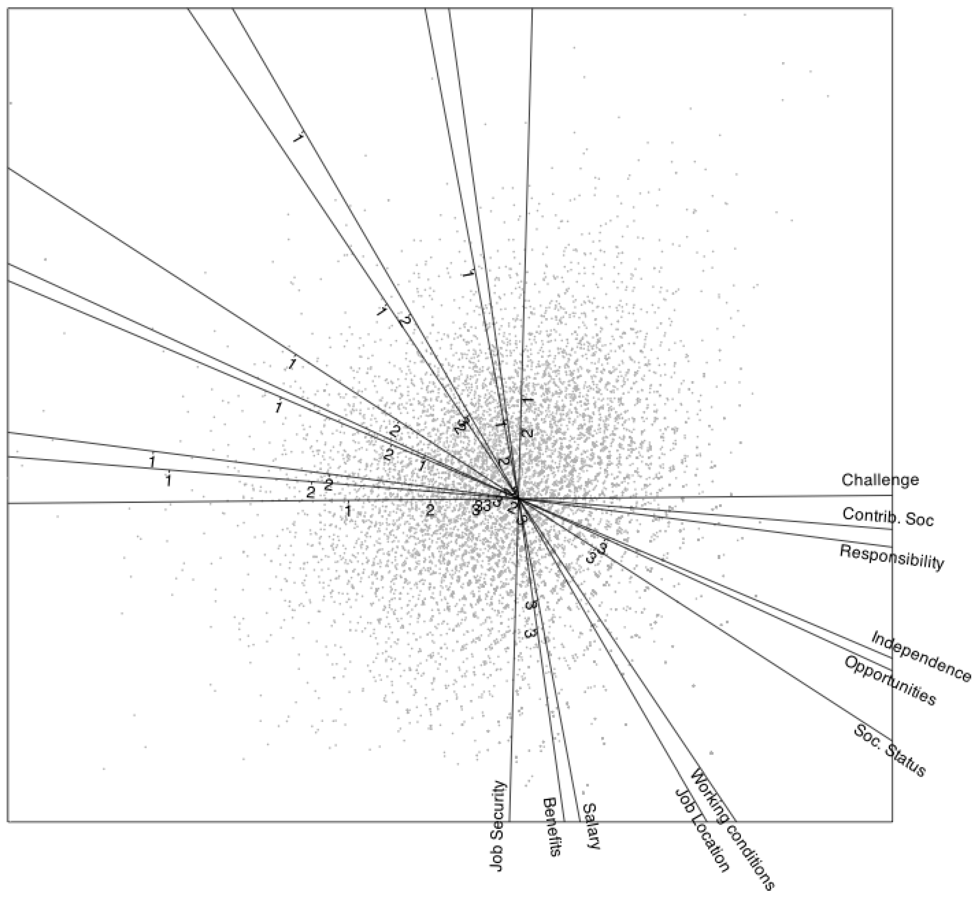
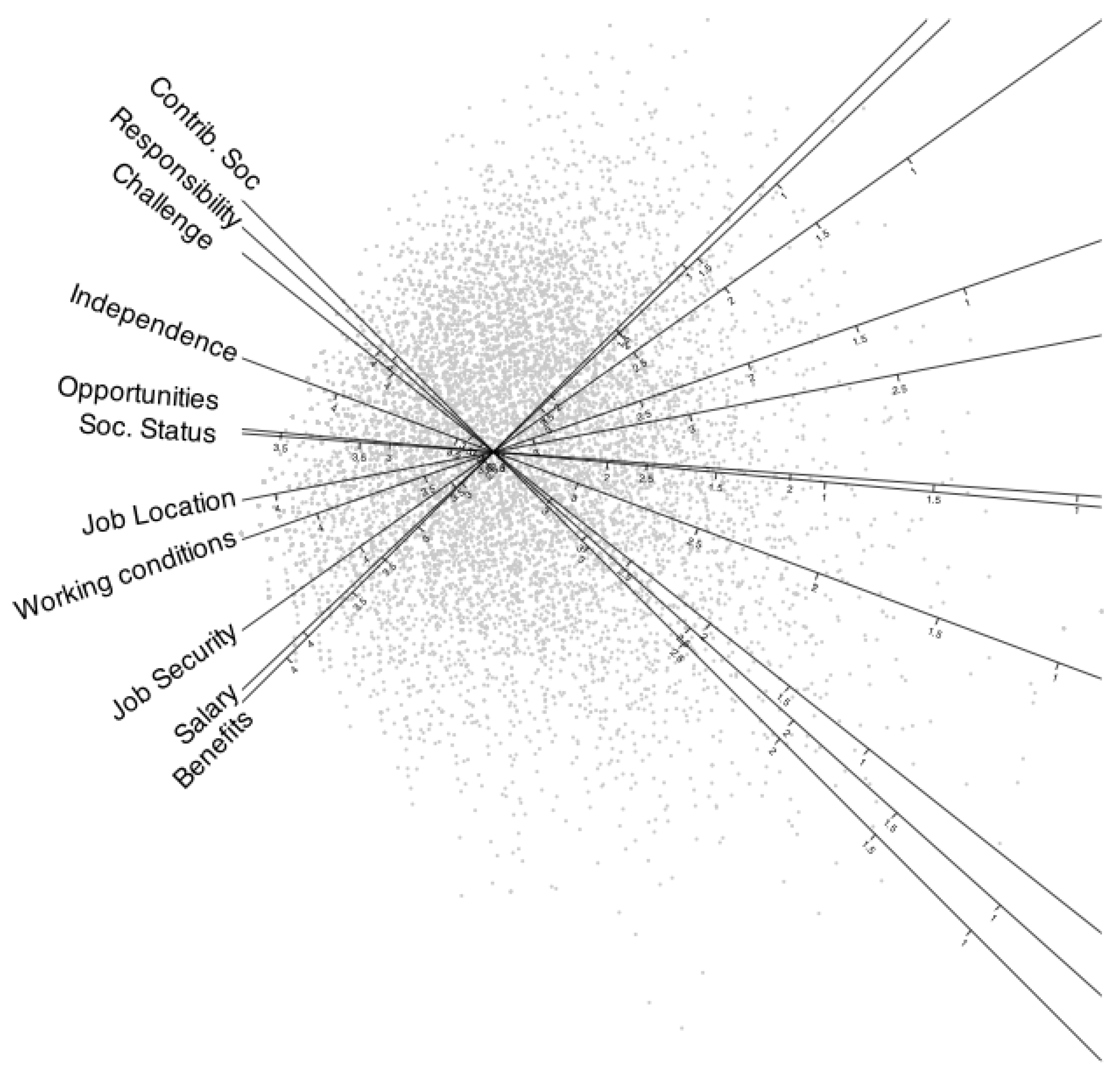
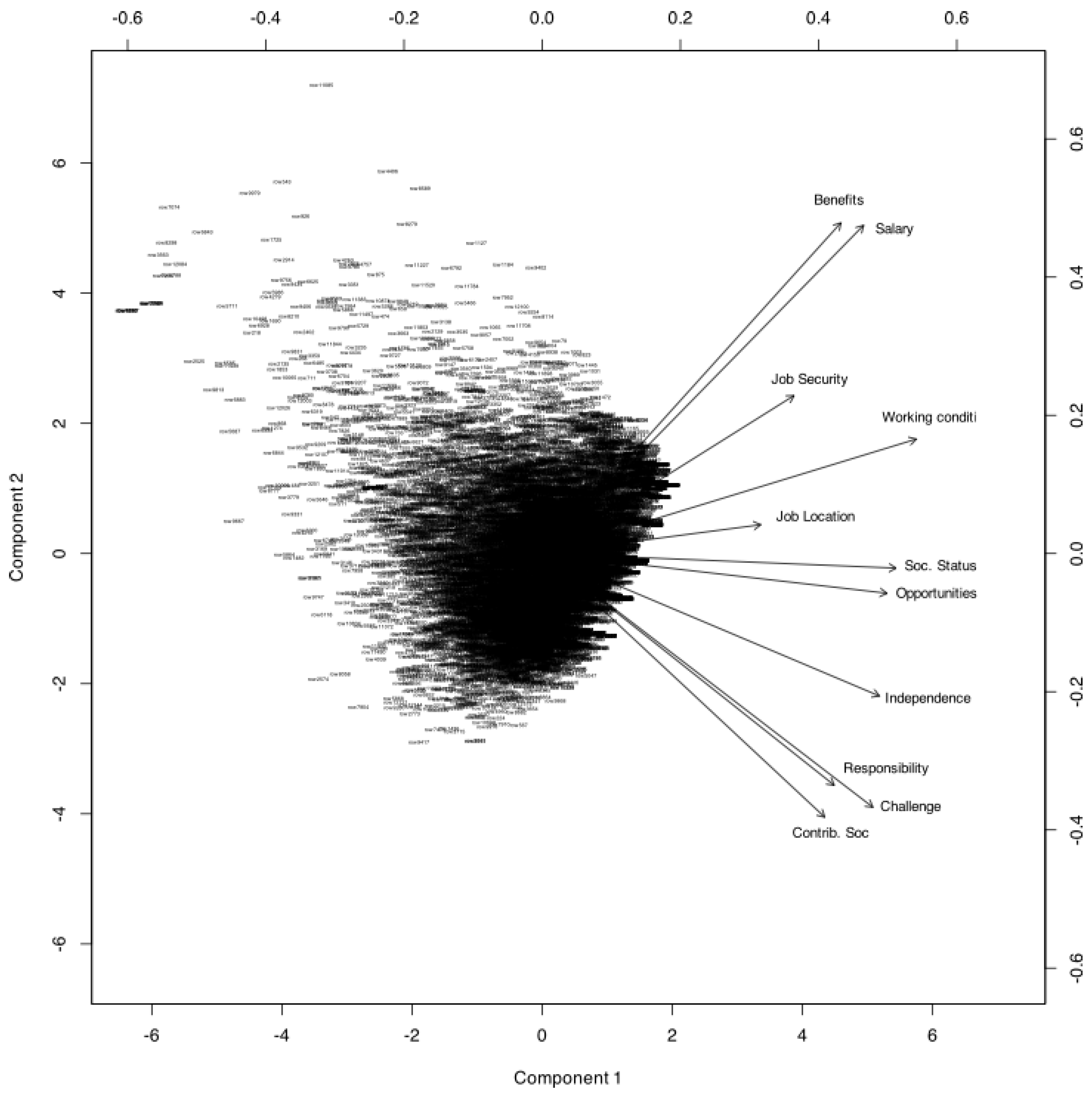
The biplot of the ordinal data is shown in Figure 8, where points represent individuals and vectors indicate the directions associated with the variables. In addition to the numerical fit measures presented earlier, graphical representations such as biplots are valuable tools for interpreting patterns in the data. Biplots allow for the simultaneous visualization of key characteristics in both individuals and variables, as well as the relationships between them.

Figure 8. Ordinal logistic biplot for the satisfaction of doctorate holders with their principal job in Spain. The labeled marks on each line are the thresholds for the separation of prediction among categories.

Although we did not initially consider our biplots within the traditional frameworks of JK (RMP) or GH (CMP) biplots, the relationship between the coordinates and factor loadings discussed in Section 3.4 indicates that the proposed biplots correspond to the GH type, in which emphasis is placed on the variables. In this type of biplot, the angles between variable directions represent correlations—specifically, polychoric correlations among ordinal variables in our case. Small acute angles indicate strong positive correlations, angles approaching ${180}^{\circ }$ suggest strong negative correlations, and right angles indicate a lack of correlation.

Some variables exhibit similar behavior—for instance, level of responsibility, intellectual challenge, and contribution to society—as reflected by the small angles between their corresponding directions. Although some groups of variables have very similar directions, the predicted category boundaries within these groups may still differ significantly. This is observed, for example, with opportunities for advancement and degree of independence.

Individual markers are represented by small dots and, to avoid visual clutter, are not labeled, as the analysis does not focus on any specific individual. In general, the distances between individual points reflect their similarity: the closer two points are, the more similar their response patterns tend to be. This graphical structure often reveals clusters of similar individuals and the variables responsible for those groupings. Clusters may also be identified using external nominal variables to assess whether the extracted dimensions are associated with known groupings.

The projection of an individual onto the direction of a variable allows for category prediction. Threshold points separating adjacent categories are marked along each variable’s direction using numeric labels. For example, a point marked “1” indicates the threshold for switching the prediction from the first to the second category, “2” indicates the threshold between the second and third categories, and so on.

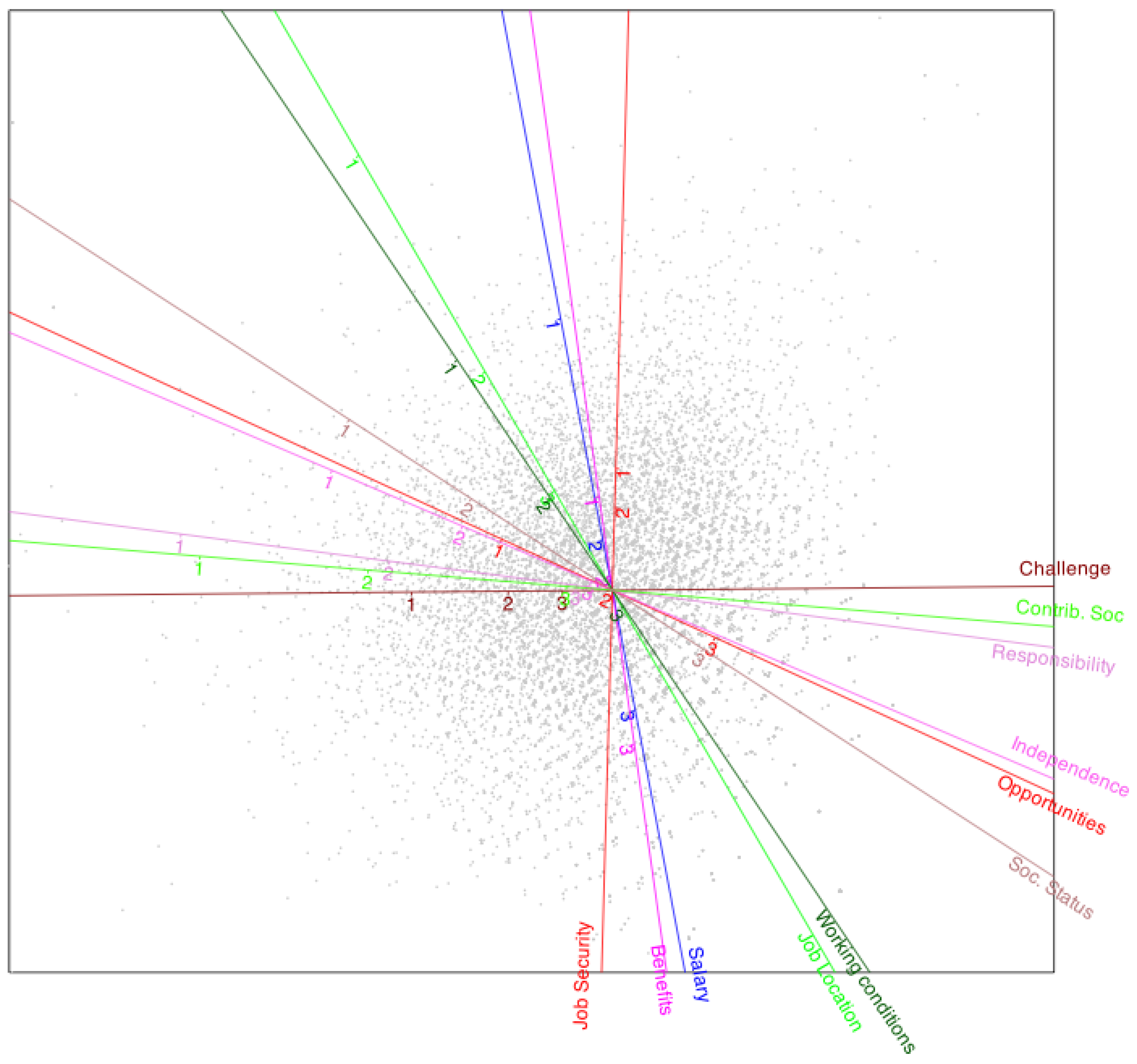
The figure may be further improved by using different colors for each variable, as shown in Figure 9. This visual aid enhances the readability of the plot and helps distinguish category thresholds for each variable.

Figure 9. Ordinal logistic biplot for the satisfaction of doctorate holders with their principal job in Spain. Variables are displayed in different colors.

All variables display three threshold marks, except for job security, which has only two (1 and 2), indicating that category 3 is never predicted. In other words, the probability of an individual falling into category 3 is never higher than that of other categories; thus, it is considered a hidden or never-predicted category.

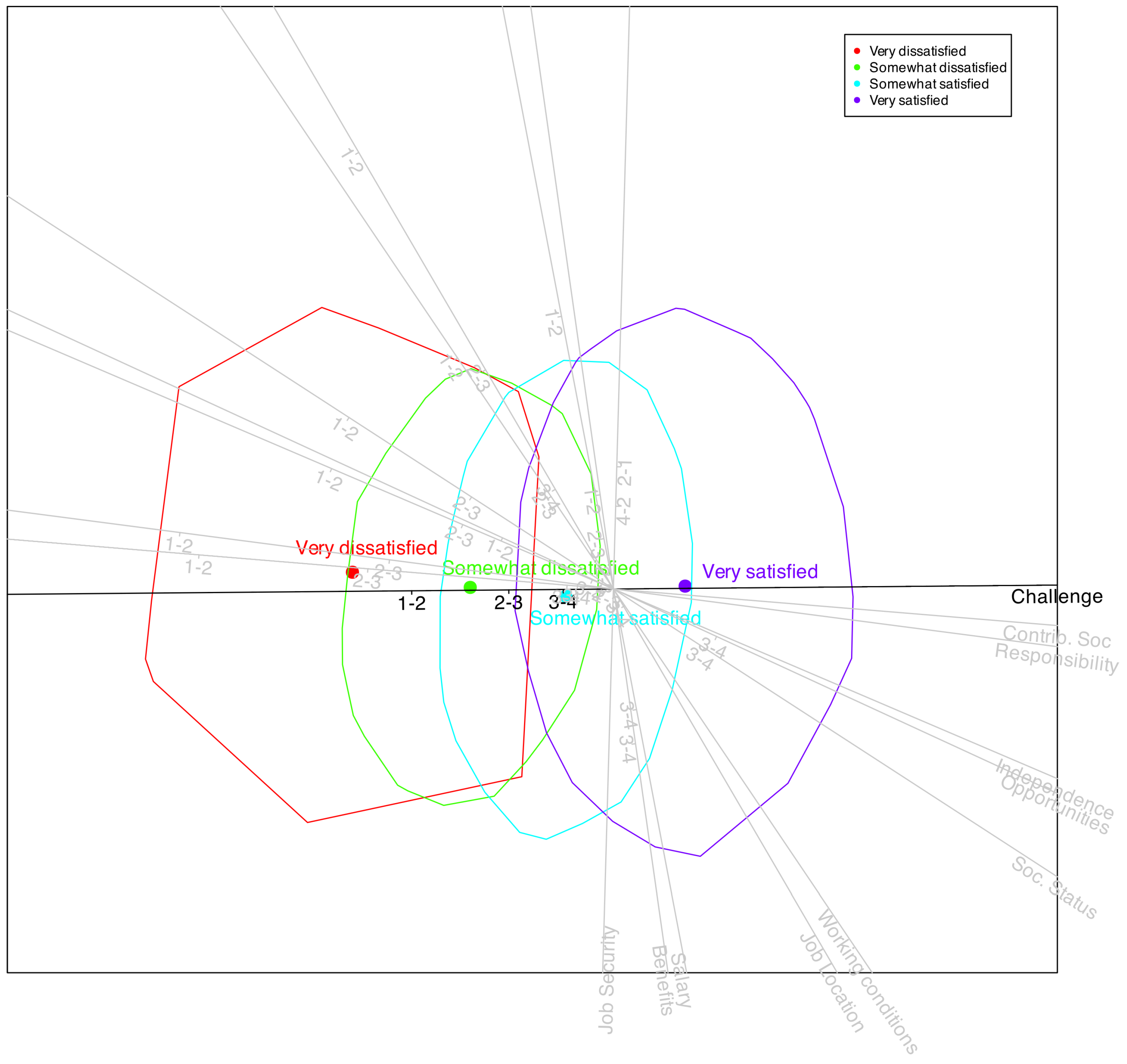
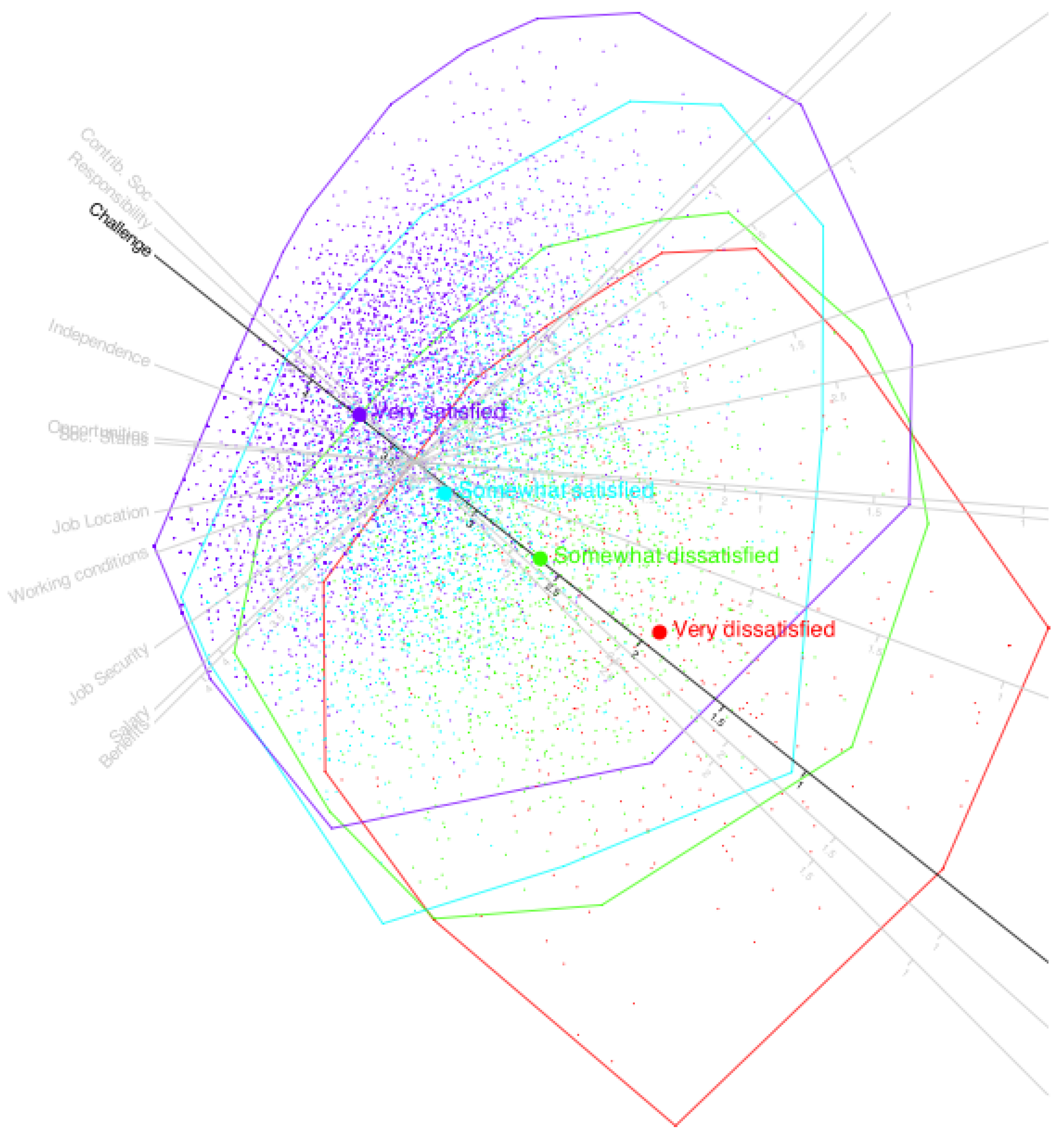
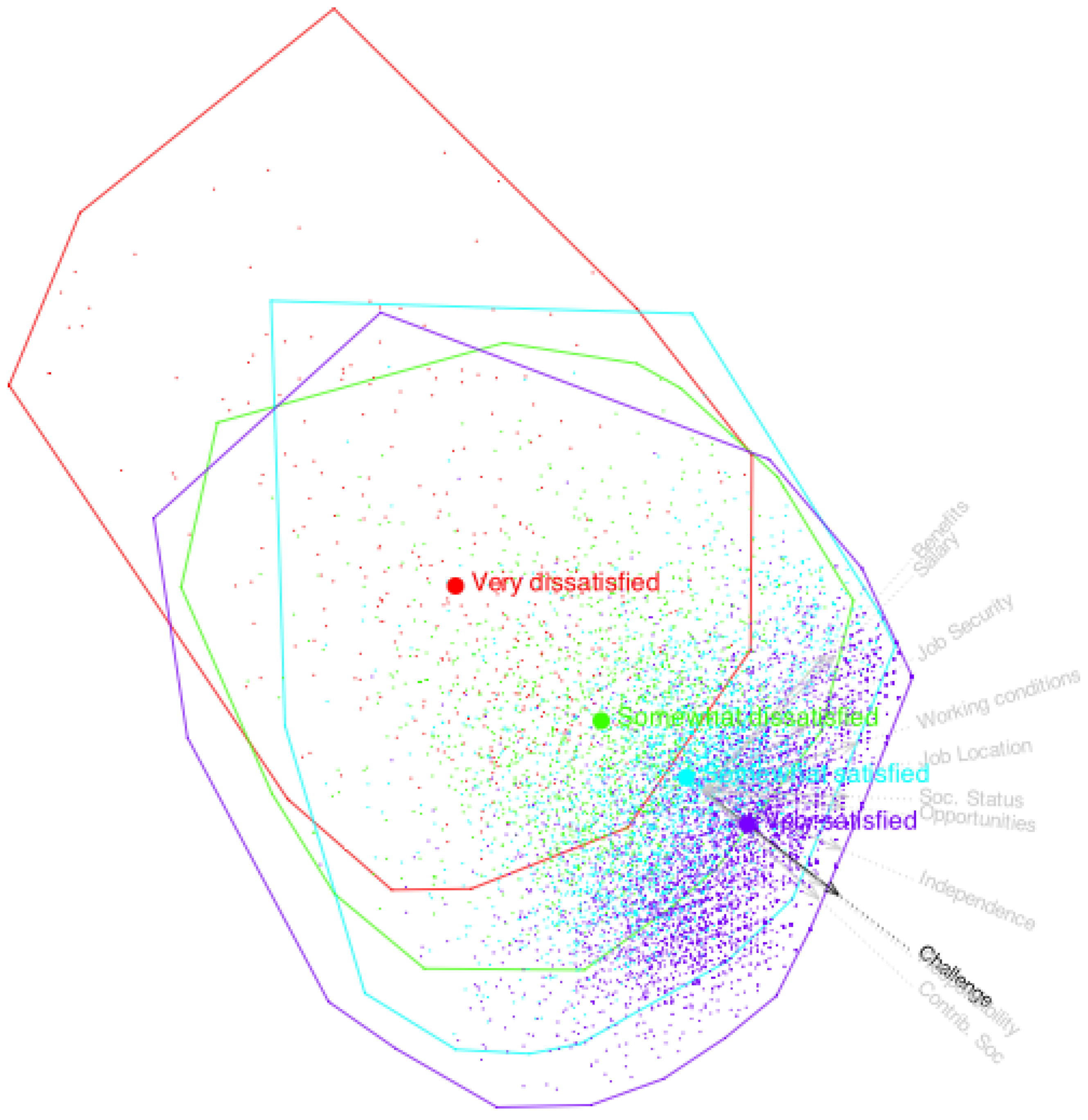
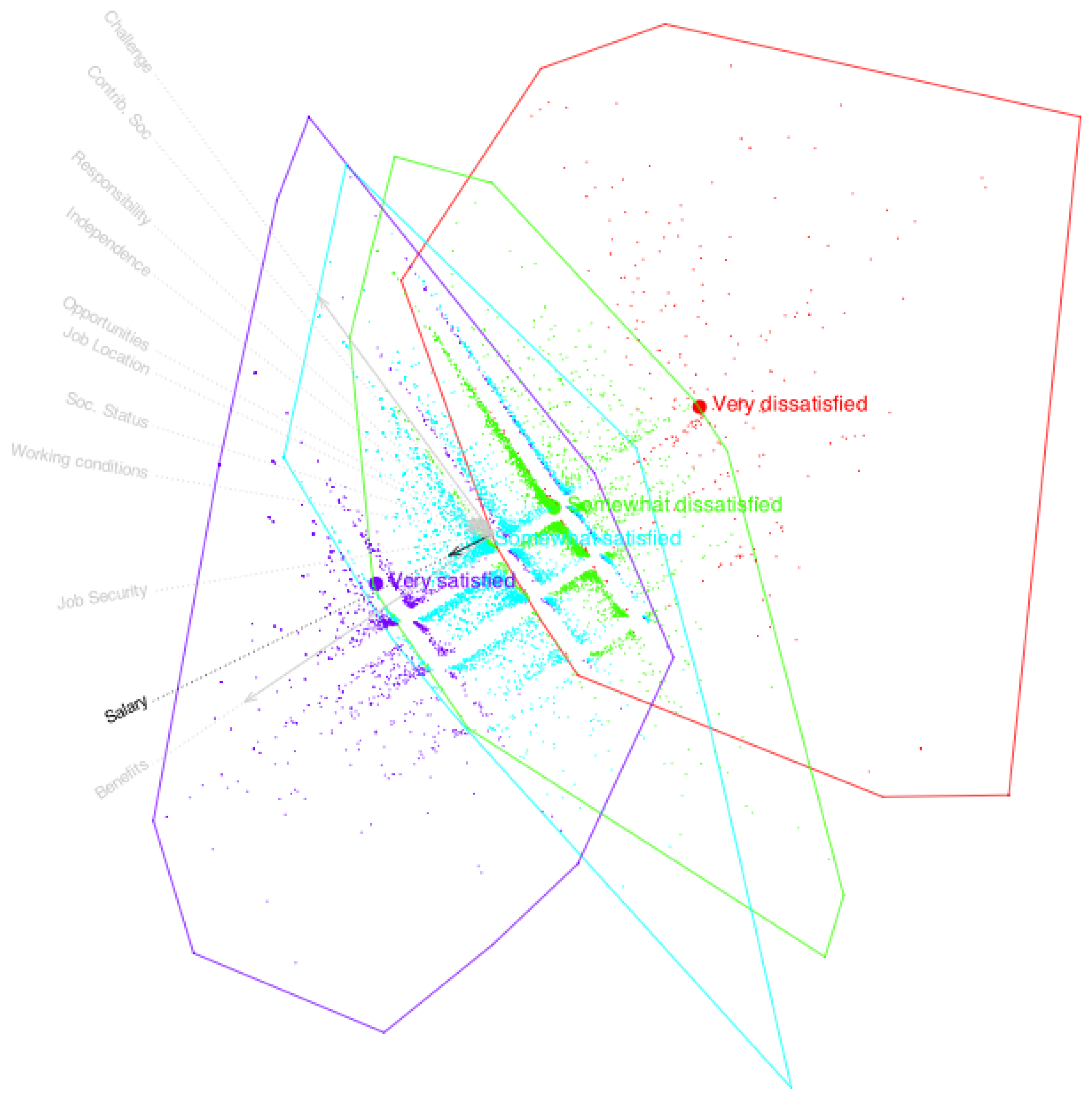
The biplot visually reflects the underlying factor structure of the dataset. To illustrate how the geometry captures the structure of a particular variable, we can enhance the plot by clustering individuals according to their observed response categories. Figure 10 shows such a representation for the variable Challenge, where individuals are colored or marked based on their observed categories. This visualization highlights how the model’s prediction boundaries align with actual response patterns.

Figure 10. The points for individuals in each observed category are covered by convex hulls in different colors. The centers of clusters are also marked.

We observe that the cluster centers are closely arranged along the direction of the variable Challenge, indicating that this axis effectively captures the underlying pattern of that variable. A similar analysis can be performed for the remaining variables, confirming that the biplot reflects the structure of all variables, albeit to different degrees. The fit indices previously discussed provide a quantitative measure of how well each variable is represented in the low-dimensional space.

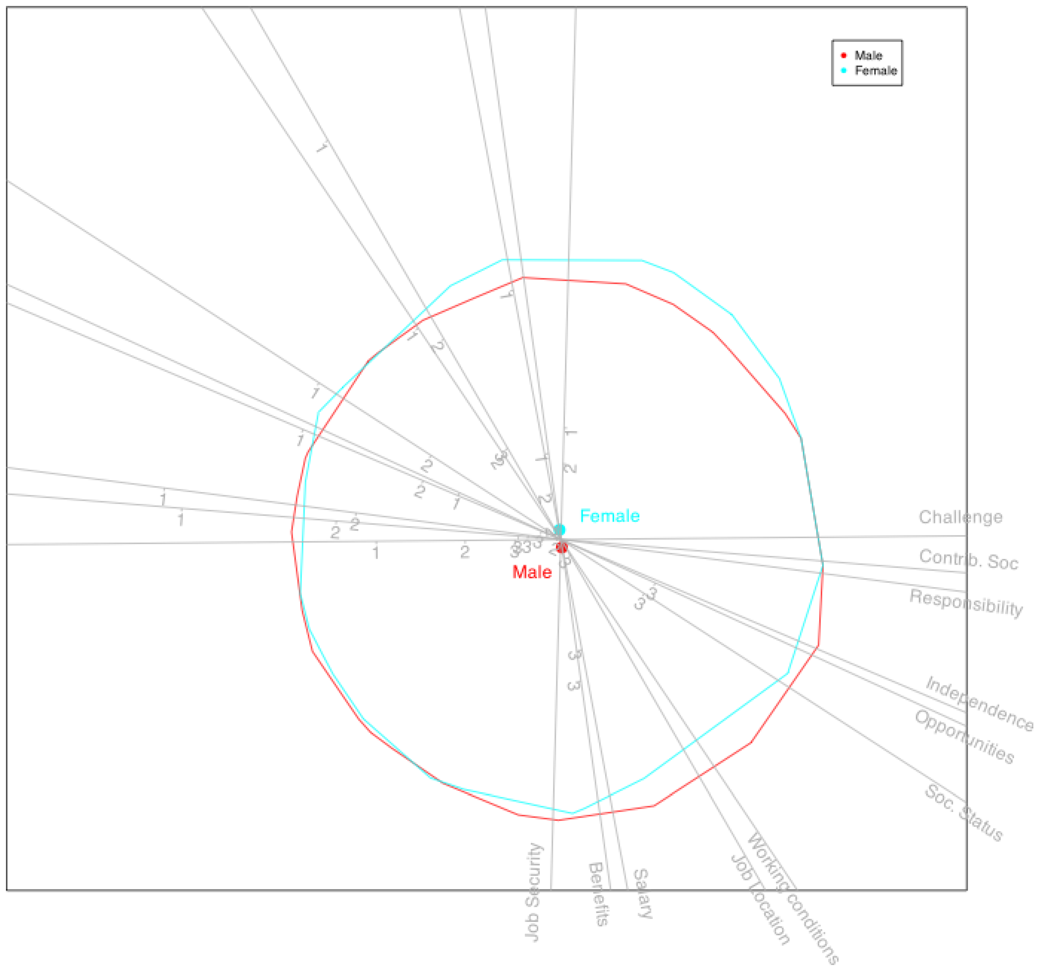
The final biplot can also be used to examine the behavior of different groups of individuals defined by external nominal variables—for example, comparing males and females to explore potential relationships between job satisfaction and gender. Figure 11 presents such a comparison.

Figure 11. Ordinal logistic biplot for the satisfaction of doctorate holders with clusters for each sex.

The positions of men and women, represented by the centroids of their coordinates on the biplot, are virtually indistinguishable (Figure 11). This suggests that there are minimal differences between male and female doctorate holders in how they perceive job satisfaction.

5. Comparison to Other Methods

In addition to our ordinal logistic biplot (OLB), we apply several alternative methods to the dataset in this section: principal component analysis (PCA), categorical principal component analysis (CATPCA), cumulative logistic principal component analysis (CLPCA), and Multidimensional Item Response Theory (MIRT).

5.1. PCA Biplot

Many applied researchers treat ordinal data as if it were measured on an interval scale and directly apply classical principal component analysis (PCA) with standardized data, followed by the corresponding biplot representation. This approach effectively performs PCA on the Pearson correlation matrix, which is not optimal for ordinal data. For instance, [49] shows that while Pearson’s r is relatively robust to mild deviations from normality, it is not robust when variables are discretely or ordinally scaled—correlations tend to shrink as the number of categories decreases. Similarly, [50] argues that treating ordinal scales as interval using Pearson’s r can yield misleading results and recommends using polychoric correlations or ordinal reliability coefficients instead.

Nevertheless, PCA remains a quick and computationally efficient exploratory technique. The classical biplot is based on singular value decomposition (SVD), making the algorithm particularly fast and accessible for initial analyses.

All calculations were performed using the MultBiplotR package [33] in the R statistical environment [34].

The variance explained by the first two components is reported in Table 4, amounting to 44.77% of the total variance.

Table 4. Explained variance (PCA biplot).

	Eigenvalue	Exp. Var	Cumulative
1	42,154.54	31.43	31.43
2	17,890.08	13.34	44.77

Table 5 presents the loadings (i.e., correlations between variables and components) and the communalities for the PCA solution. We observe that the correlations between items and dimensions are generally lower than the communalities obtained with our proposed model, the ordinal logistic biplot (OLB; see Table 2). This discrepancy is likely due to the use of Pearson correlations in PCA, which tend to underestimate the strength of associations among ordinal variables. As discussed earlier, treating ordinal data as interval-scaled introduces distortions that may affect both the accuracy of the factor structure and the interpretability of the results.

Table 5. Loadings and communalities for the PCA biplot.

	Dim 1	Dim 2	Communalities
Salary	−0.58	−0.55	0.63
Benefits	−0.54	−0.54	0.58
Job Security	−0.46	−0.32	0.31
Job Location	−0.39	−0.07	0.16
Working conditions	−0.68	−0.24	0.52
Opportunities	−0.63	0.06	0.40
Challenge	−0.59	0.47	0.56
Responsibility	−0.50	0.44	0.44
Independence	−0.60	0.23	0.42
Contrib. Soc	−0.49	0.49	0.49
Soc. Status	−0.64	0.05	0.42

The resulting biplot is shown in Figure 12. Scales have been added along each variable axis to aid in the interpretation of predicted values. These predictions are not limited to discrete values but include decimal values as well, reflecting the continuous nature of PCA scores.

Figure 12. Results of the classical PCA biplot (CMP or GH biplot) obtained with the function PCABiplot of the package MultBiplotR.

Overall, the structure revealed by the PCA is broadly consistent with previous findings. Variables such as Job Security, Salary, and Benefits cluster on one side of the plot, while Contribution to Society, Responsibility, and Challenge appear on the opposite side. These two groups of variables seem to form two largely independent factors. The remaining variables occupy intermediate positions in the biplot, with some aligning more closely with the first factor and others with the second.

The interpretability of the solution could be improved by rotating the initial factors to a more meaningful orientation. Although rotated biplots in the context of factor analysis have not been extensively discussed in the literature, this topic will be addressed in a separate study [51].

To assess how well the biplot captures the ordinal structure of the data, we augment the plot by displaying clusters of points corresponding to different observed categories—for instance, for the variable Challenge (Figure 13). This visual comparison allows us to contrast the performance of PCA with that of the ordinal logistic biplot (OLB) in representing ordinal relationships.

Figure 13. The points for individuals in each observed category of Challenge are covered by convex hulls in different colors. The centers of clusters are also marked. Obtained with the function PCABiplot of the package MultBiplotR.

The order of the group centroids is preserved; however, the individual points are more dispersed than in Figure 10, particularly at the extreme values. This suggests that the new method (OLB) provides greater resolution in capturing the ordinal structure of the variable.

In conclusion, although classical PCA is not specifically designed to model the ordinal nature of categorical data, it may still serve as a useful preliminary tool for exploratory analysis of ordinal data matrices, especially when a fast approximation is required.

5.2. Categorical PCA

Next, we apply categorical principal component analysis (CATPCA) [17] using the Gifi package [52] in the R environment [34]. CATPCA is a two-step procedure: first, a quantification step using optimal scaling, and second, a standard principal component analysis applied to the quantified variables.

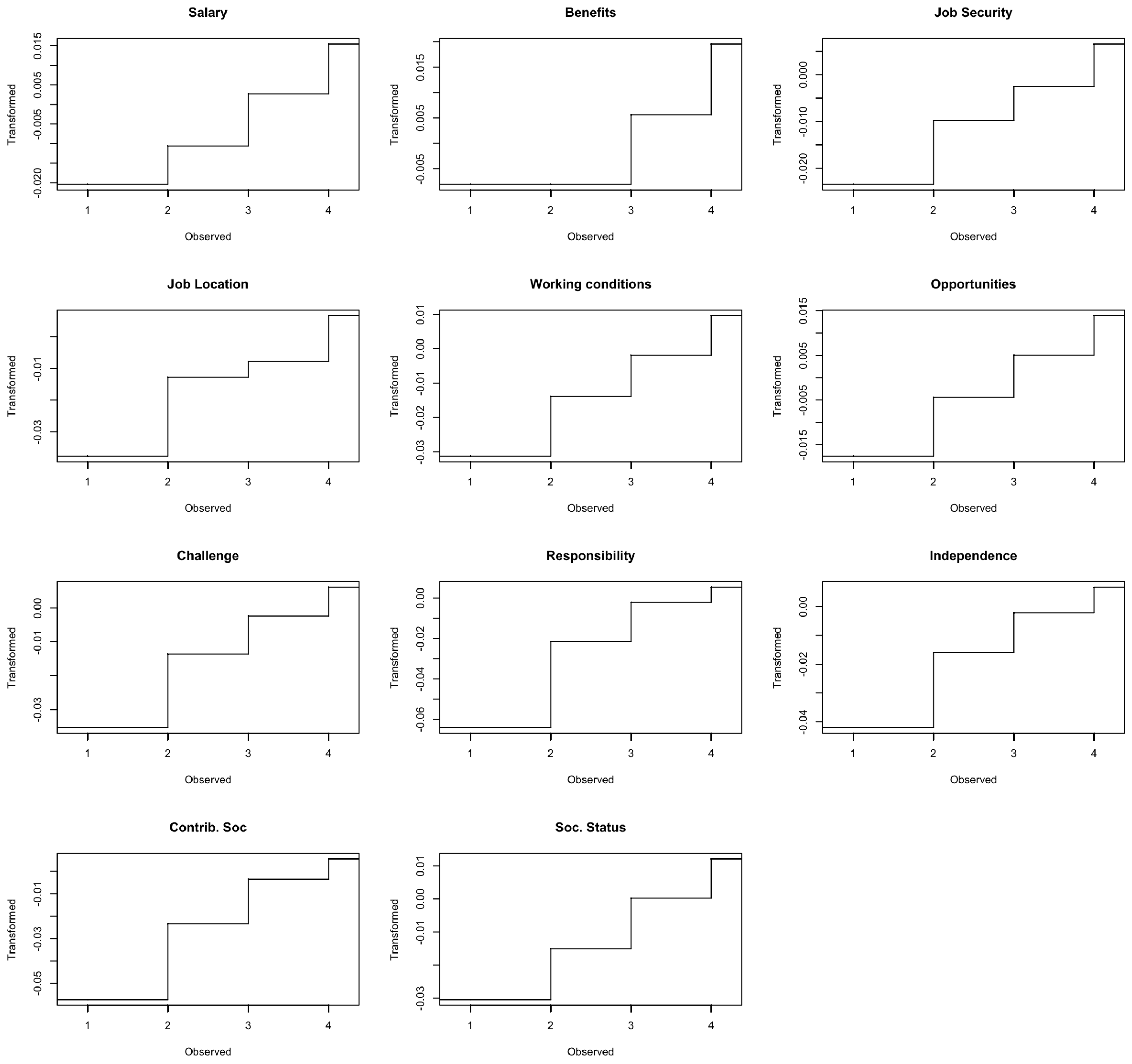
Quantification involves replacing the original ordinal values (e.g., 1, 2, 3, 4) with new, optimally scaled numeric values that preserve the ordering while maximizing variance explanation in the subsequent PCA. For example, for the variable Salary, the initial values are transformed to approximately (–0.0204, –0.0106, 0.0027, 0.0154).

The procedure also generates a transformation plot that displays the relationship between the original and transformed values (see Figure 14). These transformation plots are useful for interpreting the structure and separation of the categories for each variable and can provide insights into whether the ordinal scale behaves linearly or nonlinearly in the analysis.

Figure 14. Category quantifications obtained from the CATPCA procedure. Obtained with the package Gifi.

The amount of variance explained is shown in Table 6 and is similar to the PCA explanation.

Table 6. Explained variance (Categorical PCA).

	Eigenvalue	Exp. Var	Cumulative
1	3.5226	32.02	32.02
2	1.5246	13.86	45.88

The loadings and communalities are presented in Table 7 and are generally similar to those obtained from the classical PCA. The main difference lies in the fact that CATPCA is specifically designed to account for the ordinal nature of the data by optimally scaling the initial categorical values.

Table 7. Loadings and communalities for categorical PCA.

	D1	D2	Communalities
Salary	0.58	0.59	0.69
Benefits	0.54	0.60	0.65
Job Security	0.46	0.29	0.29
Job Location	0.40	0.05	0.16
Working conditions	0.68	0.21	0.50
Opportunities	0.62	−0.07	0.40
Challenge	0.60	−0.46	0.57
Responsibility	0.53	−0.42	0.46
Independence	0.61	−0.26	0.44
Contrib. Soc	0.51	−0.48	0.49
Soc. Status	0.64	−0.03	0.41

Although the resulting solution could potentially be rotated to enhance interpretability, this functionality is not currently supported by the software.

The method also generates a biplot, as shown in Figure 15. However, the biplot produced by the software applies different scaling to individuals and variables, which is generally discouraged, as it may distort the geometric relationships and hinder interpretability. A more appropriate biplot can be constructed using calibrated axes and supplementary graphical tools, as proposed by [53]. An improved version of this type of biplot is also discussed in [54]; however, the accompanying link to the R software implementation is no longer functional, which prevented us from reproducing their method in our analysis.

Figure 15. Biplot obtained from the CATPCA procedure using the package Gifi.

After integrating the coordinates into our package, we added clusters based on the observed categories of the variable Challenge, as in previous analyses. The resulting plot is displayed in Figure 16.

Figure 16. Biplot obtained from the CATPCA procedure with convex hulls for the categories of the variable Challenge. The figure has been obtained with the package MultBiploR using the coordinates provided by the function princals of the package Gifi.

In this version, the same scale has been applied to both rows (individuals) and columns (variables); however, the axes have been removed from the plot, as they are not necessary for interpretation in this context. As observed in the PCA case, the order of the categories is partially preserved, but considerable overlap remains among them, indicating that the ordinal structure is not fully captured.

The method does not provide additional measures of fit, such as those reported in Table 1. While analogous indices could likely be developed to assess model performance, defining such measures falls outside the scope of the present study.

5.3. Cumulative Logistic PCA

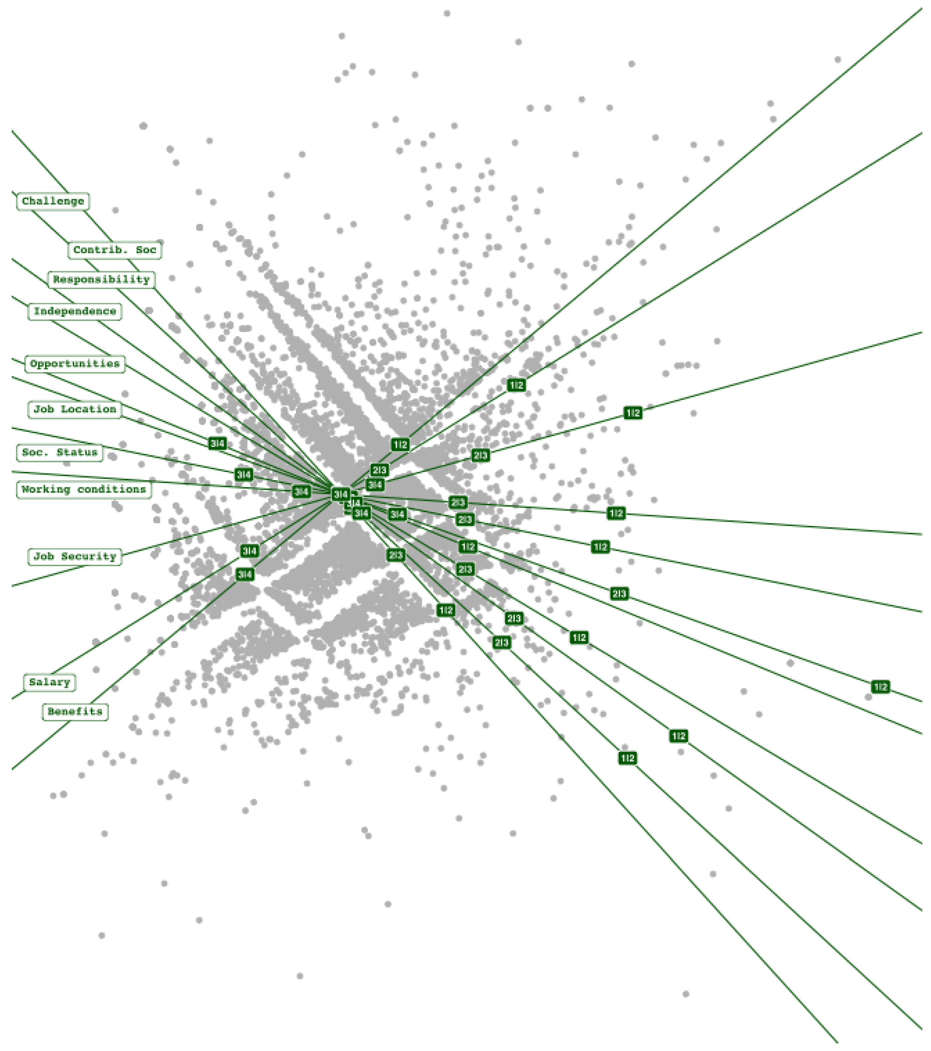
The calculations were performed using the clpca function from the lmap (Logistic Mapping) package [55]. Unlike the methods discussed previously, this package does not provide a set of loadings or communalities. Although such metrics could, in principle, be computed, they are not included in the current implementation. Instead, the package outputs a set of coordinates for the variables, which are presented in Table 8.

Table 8. Loadings and communalities for CLPCA.

	D1	D2
Salary	−2.92	−1.44
Benefits	−16.68	−11.29
Job Security	−0.85	−0.14
Job Location	−0.64	0.31
Working conditions	−1.82	0.31
Opportunities	−1.67	0.91
Challenge	−11.70	15.90
Responsibility	−0.96	0.87
Independence	−1.40	1.07
Contrib. Soc	−0.91	1.06
Soc. Status	−1.68	0.53

The coordinates provided by the CLPCA method are conceptually similar to factor loadings, although they are not directly interpretable as correlations, as is the case in traditional PCA or factor analysis. Notably, some variable coordinates are substantially larger in magnitude than others, indicating stronger associations with the latent dimensions.

To further explore these results, we refer to the graphical representation in Figure 17. The overall structure appears consistent with the findings from previously reviewed techniques—namely, the emergence of two primary dimensions: one associated with intellectual satisfaction and the other with satisfaction related to working conditions.

Figure 17. Biplot obtained from the cumulative logistic PCA procedure using the function clpca of the package lmap.

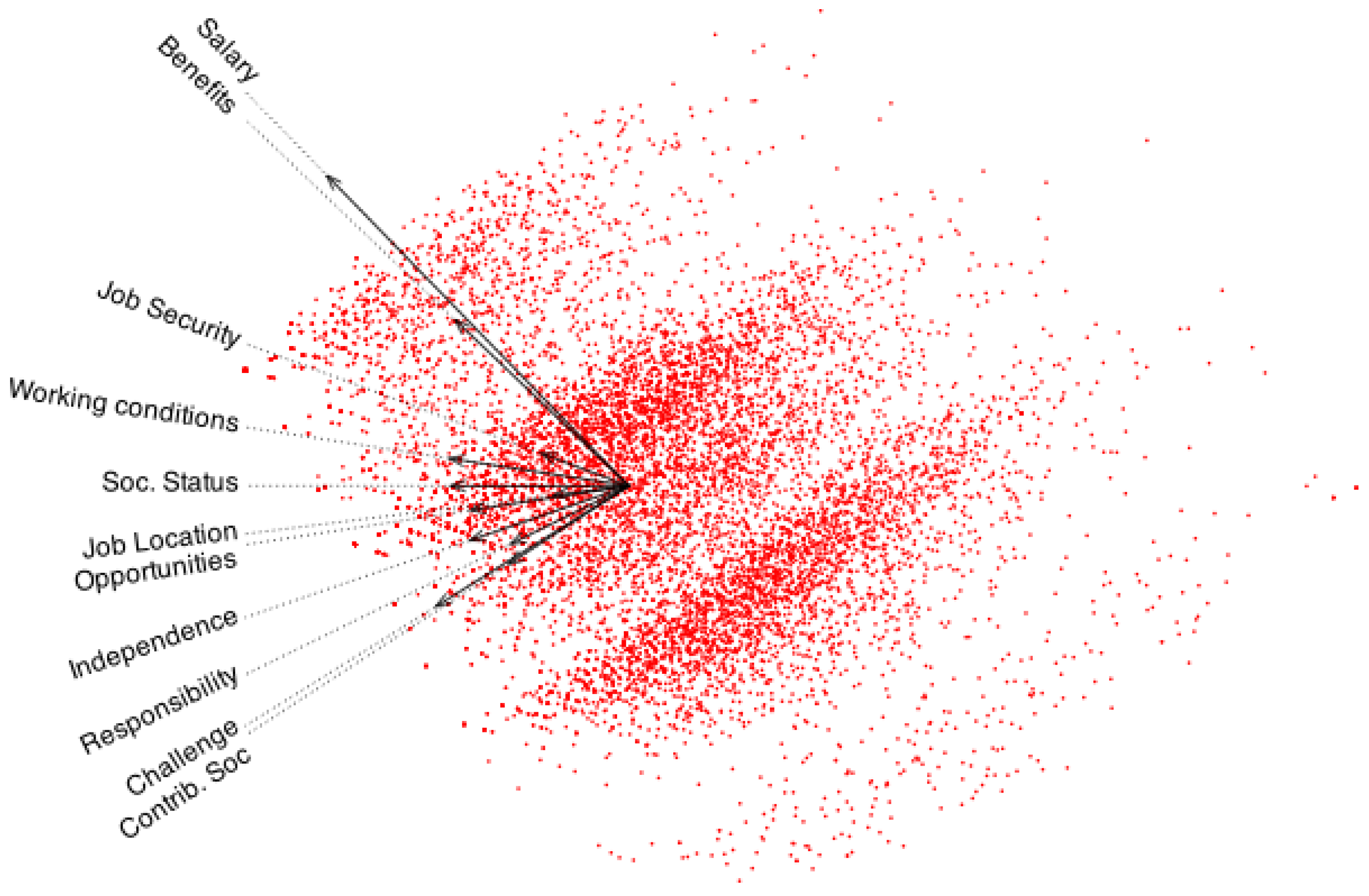
A closer inspection of the object scores reveals discrete step patterns along certain dimensions. These steps tend to align with variables that exhibit the highest coordinate values, suggesting that these variables are driving the segmentation of individuals in the reduced space.

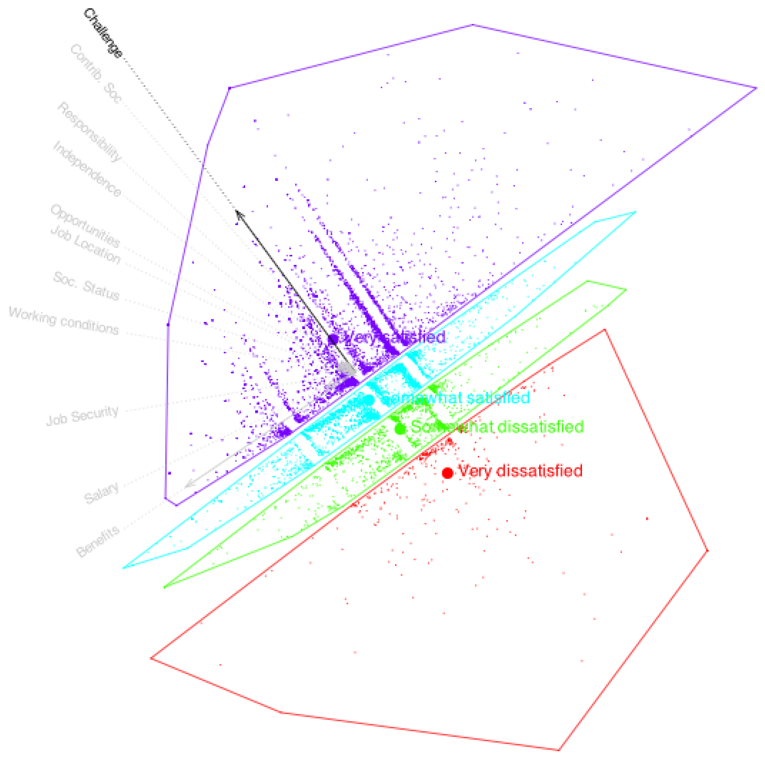
As in the previous cases, we added clusters corresponding to the observed categories of the variable Challenge, after adapting the coordinates to the biplot format implemented in our package. The resulting visualization is presented in Figure 18.

Figure 18. Biplot obtained from the cumulative logistic PCA procedure with clusters for Challenge. The figure has been obtained with the package MultBiploR using the coordinates provided by the function clpca of the package lma.

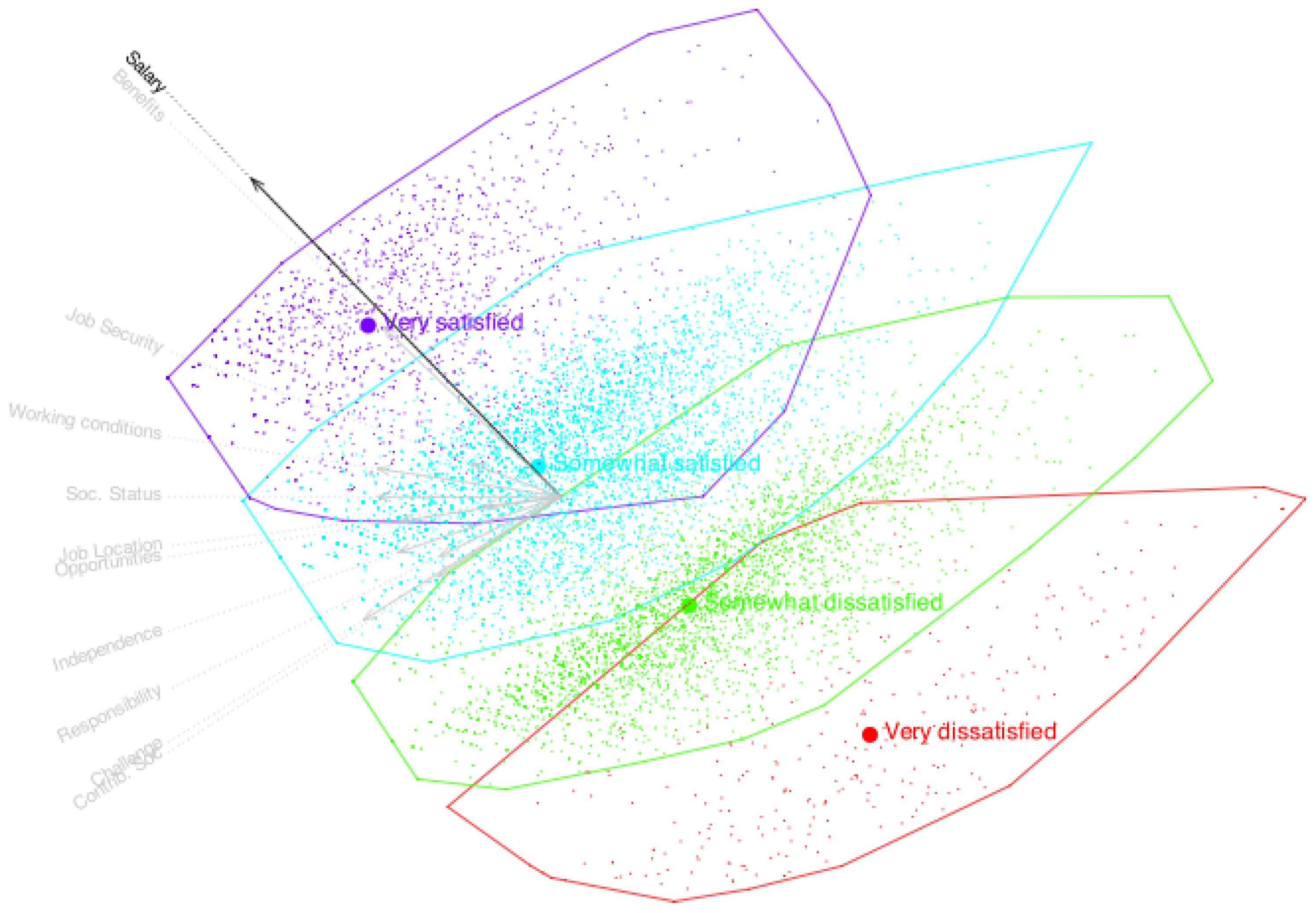
The ordinal structure of the variable Challenge is well preserved, and the model yields perfect category predictions. A similar result is observed for the variable Benefits. However, the predictive performance is notably weaker for other variables—for example, Salary, as illustrated in Figure 19.

Figure 19. Biplot obtained from the cumulative logistic PCA procedure with clusters for Salary. The figure has been obtained with the package MultBiploR using the coordinates provided by the function clpca of the package lma.

It remains unclear whether this pattern is a desirable outcome of the model or the result of a separation issue, similar to those encountered in ordinal logistic regression. In contrast, our proposed method (OLB) appears to distribute classification accuracy more evenly across variables, thereby reducing the risk of overfitting to a small subset of items.

5.4. Multidimensional Item Response Theory (MIRT)

Multidimensional Item Response Theory (MIRT) is not primarily designed for graphical representation of results; however, in principle, a biplot could be derived from its standard output. For our analysis, we employed the mirt package [56] to perform the calculations. Among other outputs, the package provides a set of loadings and communalities, which we use for comparison with the results obtained from our proposed method. A varimax rotation was applied to facilitate interpretation. The results are presented in Table 9.

Table 9. Loadings and communalities for MIRT model.

	F1	F2	Communalities
Salary	0.09	0.91	0.84
Benefits	0.11	0.77	0.61
Job Security	0.23	0.37	0.19
Job Location	0.31	0.19	0.14
Working conditions	0.47	0.50	0.47
Opportunities	0.56	0.32	0.41
Challenge	0.76	0.09	0.58
Responsibility	0.55	0.12	0.32
Independence	0.62	0.22	0.43
Contrib. Soc	0.60	0.06	0.36
Soc. Status	0.53	0.42	0.46

Although the package does not provide a biplot by default, we constructed a simplified version using the information available in the solution. The resulting biplot is presented in Figure 20.

Figure 20. Biplot obtained from the MIRT procedure. The figure has been obtained with the package MultBiploR using the coordinates provided by the function mirt of the package mirt.

A noticeable separation of individual groups is also observed along the direction of the variable Salary, which exhibits the highest communality in the model. This separation is illustrated in Figure 21. While the grouping is relatively clear, it is not as distinct as in the case of our proposed method.

Figure 21. Biplot obtained from the MIRT procedure with clusters for Salary. The figure has been obtained with the package MultBiploR using the coordinates provided by the function mirt of the package mirt.

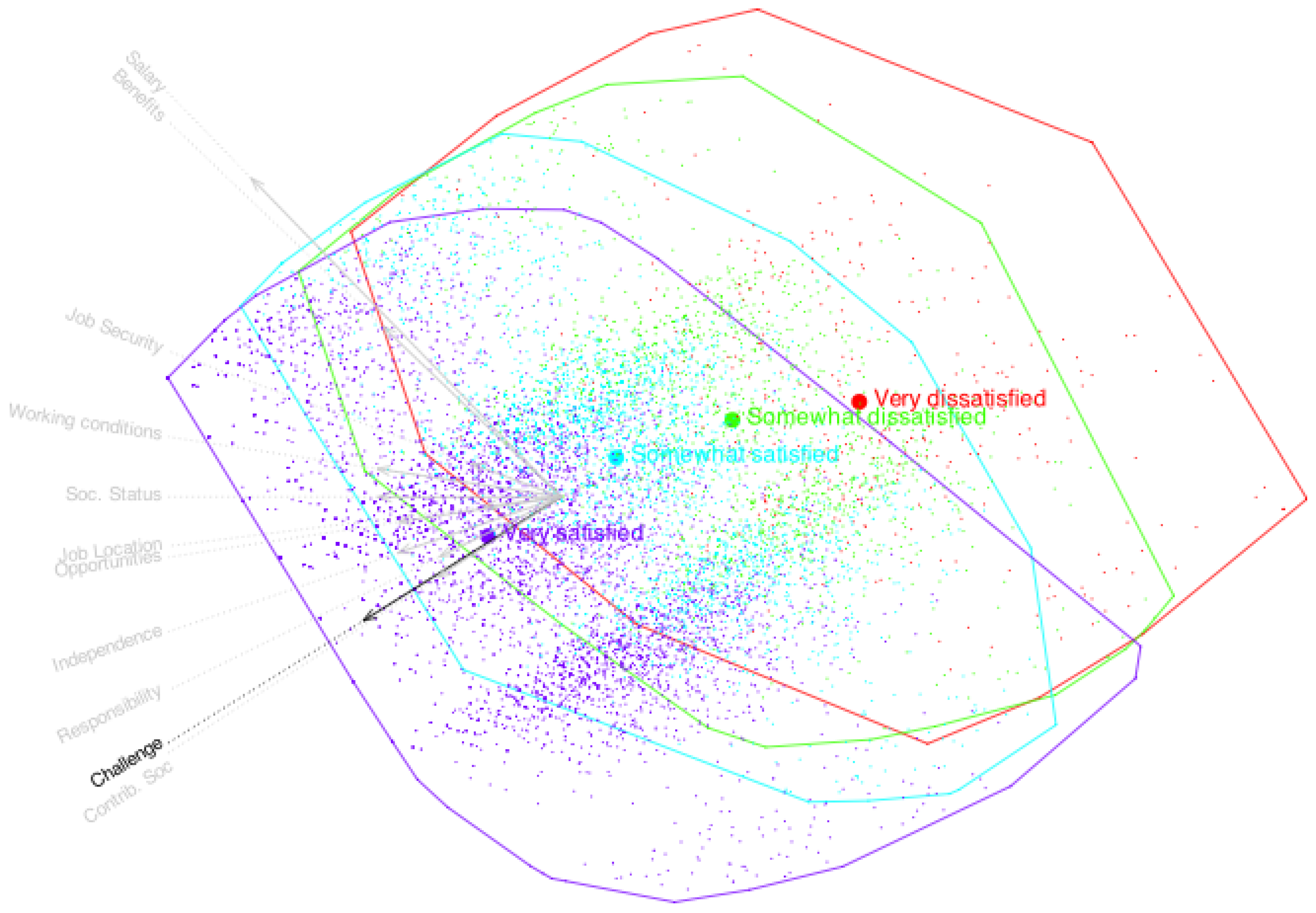
Finally, we present the clusters for the variable Challenge to facilitate comparison with the results obtained from the other techniques (Figure 22).

Figure 22. Biplot obtained from the MIRT procedure with clusters for Challenge. The figure has been obtained with the package MultBiploR using the coordinates provided by the function mirt of the package mirt.

The classification is now worse than before.

5.5. Conclusions

Among the methods considered, all except PCA have been specifically developed to handle ordinal data. Furthermore, all but PCA and CATPCA are based on logistic response models. According to the results, both CLPCA and MIRT may be affected by separation issues—a phenomenon also known in ordinal logistic regression—although further investigation is required to confirm this behavior.

The computational times were recorded using a tolerance of ${10}^{-5}$ and a maximum of 400 iterations on a Mac equipped with a 3.7 GHz Intel i5 processor (6 cores, 2019 model). A comparison of the characteristics of different methods can be seen in Table 10.

Table 10. Comparison of different methods.

	PCA	CATPCA	LCPCA	MIRT	OLB
Designed for Ordinal Data	No	Yes	Yes	Yes	Yes
Logistic Model	No	No	Yes	Yes	Yes
Explained Variance Reported	Yes	Yes	No	Yes	Yes
Loadings and Communalities	Yes	Yes	No	Yes	Yes
Allows Penalization for Separation	-	-	No	No	Yes
Biplot Reported	Yes	Yes	Yes	No	Yes
Ordinal Predictions Reported	No	No	No	No	Yes
Additional Fit Indices Reported	No	No	No	No	Yes
Time	0.3286 s	3.4279 s	10.4338 min	1.9186 min	4.708 min

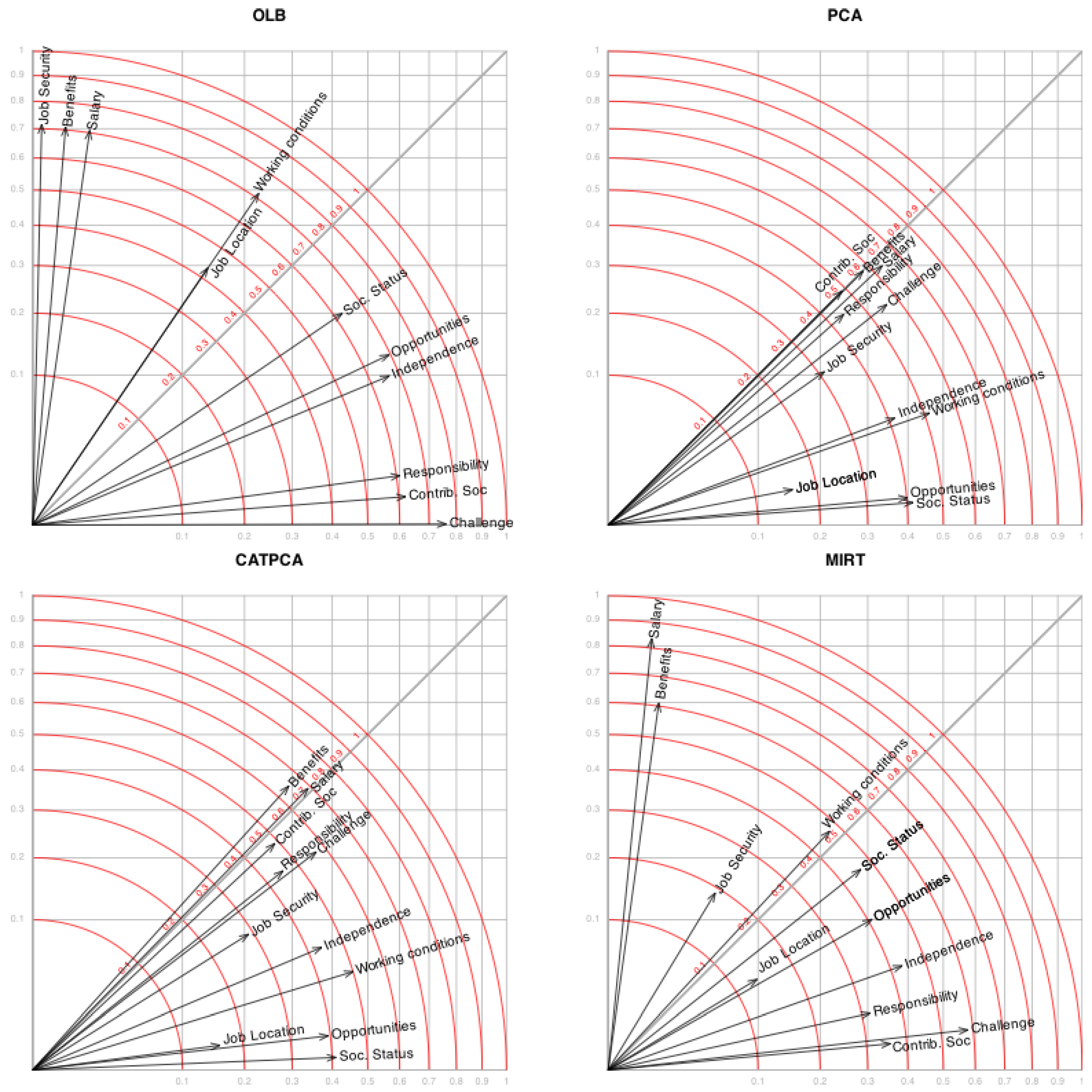
Finally, we computed a set of discrimination measures, referred to as contributions, analogous to those used in factor analysis. These represent the squared correlations between each item and the latent dimensions. The sum of contributions across dimensions corresponds to the communalities. Figure 23 displays the contribution plots. The projection of each arrow onto an axis indicates the contribution of that axis, while the circles represent either the communalities (i.e., the total contribution across both axes) or the combined contribution of the two dimensions. The grid and reference circles have been adjusted to reflect the squared correlation scale. These contributions may also be interpreted as the proportion of variance in each variable explained by the latent dimensions or, equivalently, as a measure of discriminatory power.

Figure 23. Contributions calculated for the different methods we have used.

All the methods examined produced broadly similar results in terms of the interpretation of the latent structure. In all cases, two underlying factors emerged—one associated with intellectual satisfaction and the other with working conditions—although the clarity of this separation varied across methods. As observed in the contribution plots, our proposed method, the ordinal logistic biplot (OLB), demonstrates higher discriminant power than any of the alternatives, likely due to its robustness against separation issues through the use of a quadratic (Ridge) penalization.

The current proposal is based on the assumption of proportional odds. In future work, we intend to explore alternative modeling frameworks that relax this assumption, such as the Partial Proportional Odds Model (PPOM), the Generalized Ordered Logit Model, or other ordinal models including Adjacent-Category and Continuation-Ratio formulations. These approaches may lead to new variants of the biplot tailored to different data-generating processes.

In summary, the ordinal logistic biplot (OLB) demonstrated strong performance in capturing the latent structure of ordinal satisfaction data, offering interpretable dimensions, well-separated categories, and balanced classification accuracy across variables. Classical PCA, while not designed for ordinal data, served as a rapid exploratory tool, although it tended to underestimate relationships because of its reliance on Pearson correlations. CATPCA, which incorporates optimal scaling, offered improvements over PCA but lacked fit measures and yielded less precise graphical representations. CLPCA and MIRT, both grounded in logistic response models, provided more robust theoretical frameworks for ordinal data; however, their results revealed signs of potential separation issues that may limit generalizability and require further investigation. Overall, the OLB combines methodological rigor with clear visual interpretation, positioning it as a competitive and informative approach for the exploratory analysis of ordinal multivariate data.

6. Software Note

The procedures in this paper will be added to Version 25.11 of the package MultBiplotR ([33]) developed in the R language ([34]). The package is also available from the corresponding author.

References

- Gabriel, K. The biplot graphic display of matrices with application to principal component analysis. Biometrika 1971, 58, 453–467. [Google Scholar] [CrossRef]
- Gower, J.; Hand, D. Biplots. In Monographs on Statistics and Applied Probability. 54; Chapman and Hall: London, UK, 1996; 277p. [Google Scholar]
- Gabriel, K.R.; Zamir, S. Lower rank approximation of matrices by least squares with any choice of weights. Technometrics 1979, 21, 489–498. [Google Scholar] [CrossRef]
- Gabriel, K.R. Generalised bilinear regresion. Biometrika 1998, 85, 689–700. [Google Scholar] [CrossRef]
- de Leeuw, J. Principal component analysis of binary data by iterated singular value decomposition. Comput. Stat. Data Anal. 2006, 50, 21–39. [Google Scholar] [CrossRef]
- Lee, S.; Huand, J.; Hu, J. Sparse logistic principal component analysis for binary data. Ann. Appl. Stat. 2010, 4, 21–39. [Google Scholar] [CrossRef]
- Vicente-Villardon, J.; Galindo, M.; Blazquez-Zaballos, A. Logistic Biplots. In Multiple Correspondence Analysis and Related Methods; Chapman and Hall: Boca Ratón, FL, USA, 2006; pp. 503–521. [Google Scholar]
- Demey, J.; Vicente-Villardón, J.L.; Galindo, M.P.; Zambrano, A. Identifying molecular markers associated with classification of genotypes using external logistic biplots. Bioinformatics 2008, 24, 2832–2838. [Google Scholar] [CrossRef] [PubMed]
- Vicente-Galindo, P.; de Noronha Vaz, T.; Nijkamp, P. Institutional capacity to dynamically innovate: An application to the portuguese case. Technol. Forecast. Soc. Change 2011, 78, 3–12. [Google Scholar] [CrossRef]
- Gallego, I.; Vicente-Villardon, J.L. Analysis of environmental indicators in international companies by applying the logistic biplot. Ecol. Indic. 2012, 23, 250–261. [Google Scholar] [CrossRef]
- Cañueto, J.; Cardeñoso-Álvarez, E.; García-Hernández, J.; Galindo-Villardón, P.; Vicente-Galindo, P.; Vicente-Villardón, J.; Alonso-López, D.; De Las Rivas, J.; Valero, J.; Moyano-Sanz, E.; et al. Micro rna (mir)-203 and mir-205 expression patterns identify subgroups of prognosis in cutaneous squamous cell carcinoma. Br. J. Dermatol. 2017, 177, 168–178. [Google Scholar] [CrossRef]
- Gallego-Alvarez, I.; Ortas, E.; Vicente-Villardón, J.L.; Álvarez Etxeberria, I. Institutional constraints, stakeholder pressure and corporate environmental reporting policies. Bus. Strategy Environ. 2017, 26, 807–825. [Google Scholar] [CrossRef]
- Song, Y.; Westerhuis, J.A.; Smilde, A.K. Logistic principal component analysis via non-convex singular value thresholding. Chemom. Intell. Lab. Syst. 2020, 204, 104089. [Google Scholar] [CrossRef]
- Babativa-Márquez, J.G.; Vicente-Villardón, J.L. Logistic biplot by conjugate gradient algorithms and iterated svd. Mathematics 2021, 9, 2015. [Google Scholar] [CrossRef]
- Hernández-Sánchez, J.C.; Vicente-Villardón, J.L. Logistic biplot for nominal data. Adv. Data Anal. Classif. 2017, 11, 307–326. [Google Scholar] [CrossRef]
- Vicente-Villardon, J.L.; Sanchez, J.C.H. Logistic biplots for ordinal data with an application to job satisfaction of doctorate degree holders in spain. arXiv 2014, arXiv:1405.0294. [Google Scholar] [CrossRef]
- Gifi, A. Nonlinear Multivariate Analysis; Wiley: Chichester, UK, 1990; Volume 1. [Google Scholar]
- Meulman, J.J.; Van der Kooij, A.J.; Heiser, W.J. Principal Components Analysis with Nonlinear Optimal Scaling Transformations for Ordinal and Nominal Data; Sage: Thousand Oaks, CA, USA, 2004; pp. 49–70. [Google Scholar]
- Linting, M.; Meulman, J.J.; Groenen, P.J.; Van Der Koojj, A.J. Nonlinear principal components analysis: Introduction and application. Psychol. Methods 2007, 12, 336. [Google Scholar] [CrossRef]
- Baker, F. Item Response Theory. Parameter Estimation Techniques; Marcel Dekker: New York, NY, USA, 1992. [Google Scholar]
- Bonifay, W. Multidimensional Item Response Theory; Sage Publications: Thousand Oaks, CA, USA, 2019. [Google Scholar]
- Bock, R.; Aitkin, M. Marginal maximum likelihood estimation of item parameters: Application of an em algorithm. Psychometrika 1981, 46, 443–459. [Google Scholar] [CrossRef]
- Drasgow, F. Polychoric and Polyserial Correlations; Wiley: Hoboken, NJ, USA, 2004. [Google Scholar]
- Olsson, U. Maximum likelihood estimation of the polychoric correlation coefficient. Psychometrika 1979, 44, 443–460. [Google Scholar] [CrossRef]
- Holgado-Tello, F.P.; Chacón-Moscoso, S.; Barbero-García, I.; Vila-Abad, E. Polychoric versus pearson correlations in exploratory and confirmatory factor analysis of ordinal variables. Qual. Quant. 2010, 44, 153–166. [Google Scholar] [CrossRef]
- de Rooij, M.; Breemer, L.; Woestenburg, D.; Busing, F. Logistic multidimensional data analysis for ordinal response variables using a cumulative link function. Psychometrika 2025, 90, 833–869. [Google Scholar] [CrossRef]
- Gabriel, K.R.; Galindo, M.P.; Vicente-Villardon, J.L. Use of Biplots to Diagnose Independence Models in Contingency Tables; Academic Press: Cambridge, MA, USA, 1998; pp. 391–404. [Google Scholar]
- Hand, D.J.; Daly, F.; Lunn, A.D.; McConway, K.J.; Ostrowski, E. A Handbook of Small Data Sets; CRC Press: Boca Raton, FL, USA, 1994. [Google Scholar]
- Gabriel, K.R. Biplot Display of Multivariate Matrices for Inspection of Data and Diagnosis; Technical Report; University of Rochester: Rochester, NY, USA, 1980. [Google Scholar]
- Gardner-Lubbe, S.; Le Roux, N.; Gower, J. Measures of fit in principal component and canonical variate analyses. J. Appl. Stat. 2008, 35, 947–965. [Google Scholar] [CrossRef]
- Vicente-Villardón, J.L. Multbiplot: A Package for Multivariate Analysis Using Biplots; University of Salamanca, Department of Statistics: Salamanca, Spain, 2010. [Google Scholar]
- Vicente-Gonzalez, L.; Vicente-Villardon, J.L. Partial least squares regression for binary responses and its associated biplot representation. Mathematics 2022, 10, 2580. [Google Scholar] [CrossRef]
- Vicente-Villardon, J.L.; Vicente-Gonzalez, L.; Frutos-Bernal, E. MultBiplotR: Multivariate Analysis Using Biplots in R; R Package Version 23.08.1; Universidad de Salamanca: Salamanca, Spain, 2023. [Google Scholar]
- R Core Team. R: A Language and Environment for Statistical Computing; R Foundation for Statistical Computing: Vienna, Austria, 2021. [Google Scholar]
- Babativa-Márquez, J.G. BiplotML: Biplots Estimation with Machine Learning Algorithms, 2020.
- Samejima, F. Estimation of latent ability using a response pattern of graded scores. Psychometrika 1969, 34, 1–97. [Google Scholar] [CrossRef]
- Koenker, R.; Bassett, G. Regressions quantiles. Econometrica 1978, 46, 33–50. [Google Scholar] [CrossRef]
- Heinze, G.; Schemper, M. A solution to the problem of separation in logistic regression. Stat. Med. 2002, 21, 2409–2419. [Google Scholar] [CrossRef]
- le Cessie, S.; van Houwelingen, J.C. Ridge estimators in logistic regression. J. R. Stat. Soc. Ser. C (Appl. Stat.) 1992, 41, 191–201. [Google Scholar] [CrossRef]
- Jöreskog, K.G.; Moustaki, I. Factor analysis of ordinal variables: A comparison of three approaches. Multivar. Behav. Res. 2001, 36, 347–387. [Google Scholar] [CrossRef]
- Mair, P.; Reise, S.P.; Bentler, P. IRT Goodness-of-Fit Using Approaches from Logistic Regression; UCLA Statistics Preprint Series, 540; UCLA: Los Angeles, CA, USA, 2008. [Google Scholar]
- Gabriel, K.R. Goodness of fit of biplots and correspondence analysis. Biometrika 2002, 89, 423–436. [Google Scholar] [CrossRef]
- la Grange, A.; le Roux, N.; Gardner-Lubbe, S. Biplotgui: Interactive biplots in R. J. Stat. Softw. 2009, 30, 1–37. [Google Scholar] [CrossRef]
- Benzecri, J.P. L’Analyse des Donnees; Dunod: Paris, France, 1976. [Google Scholar]
- Greenacre, M.J. Theory and Applications of Correspondence Analysis; Academic Press: Cambridge, MA, USA, 1984. [Google Scholar]
- Galindo-Villardon, M.P. Una alternativa de representacion simultanea: Hj-biplot. Questiio 1986, 10, 13–23. [Google Scholar]
- Long, J.S.; Freese, J. Regression Models for Categorical Dependent Variables Using Stata, 3rd ed.; Stata Press: College Station, TX, USA, 2014. [Google Scholar]
- Schwabe, M. The careers paths of doctoral graduates in Austria. Eur. J. Educ. 2011, 46, 153–168. [Google Scholar] [CrossRef]
- Havlicek, L.L.; Peterson, N.L. Robustness of the Pearson correlation against violations of assumptions. Percept. Mot. Ski. 1976, 43, 1319–1334. [Google Scholar] [CrossRef]
- Gadermann, A.M.; Guhn, M.; Zumbo, B.D. Estimating ordinal reliability for likert-type and ordinal item response data: A conceptual, empirical, and practical guide. Pract. Assess. Res. Eval. 2012, 17, n3. [Google Scholar]
- Valdes-Rodriguez, M.; Vicente-Gonzalez, L.; Vicente-Villardon, J.L. Factor analysis biplots for continuous, binary and ordinal data. Preprints 2025. [Google Scholar]
- Mair, P.; De Leeuw, J. Gifi: Multivariate Analysis with Optimal Scaling, R package version 1.0-0. 2025.
- Blasius, J.; Eilers, P.H.; Gower, J. Better biplots. Comput. Stat. Data Anal. 2009, 53, 3145–3158. [Google Scholar] [CrossRef]
- Gower, J.C.; Le Roux, N.J.; Gardner-Lubbe, S. Biplots: Quantitative data. Wiley Interdiscip. Rev. Comput. Stat. 2015, 7, 42–62. [Google Scholar] [CrossRef]
- de Rooij, M.; Busing, F.; Claramunt Gonzalez, J. lmap: Logistic Mapping, R package version 0.2.4. 2025.
- Chalmers, R.P. mirt: A multidimensional item response theory package for the R environment. J. Stat. Softw. 2012, 48, 1–29. [Google Scholar] [CrossRef]
Disclaimer/Publisher’s Note: The statements, opinions and data contained in all publications are solely those of the individual author(s) and contributor(s) and not of MDPI and/or the editor(s). MDPI and/or the editor(s) disclaim responsibility for any injury to people or property resulting from any ideas, methods, instructions or products referred to in the content. |
© 2025 by the authors. Licensee MDPI, Basel, Switzerland. This article is an open access article distributed under the terms and conditions of the Creative Commons Attribution (CC BY) license (https://creativecommons.org/licenses/by/4.0/).