Abstract
Currently, thermal power units undertake the task of peak and frequency regulation, and their internal equipment is in a non-conventional environment, which could very easily fail and thus lead to unplanned shutdown of the unit. To realize the condition monitoring and early warning of the key equipment inside coal power units, this study proposes a deep learning-based equipment condition anomaly detection model, which combines the deep autoencoder (DAE), Transformer, and Gaussian mixture model (GMM) to establish an anomaly detection model. DAE and the Transformer encoder extract static and time-series features from multi-dimensional operation data, and GMM learns the feature distribution of normal data to realize anomaly detection. Based on the data verification of boiler superheater equipment and turbine bearings in real power plants, the model is more capable of detecting equipment anomalies in advance than the traditional method and is more stable with fewer false alarms. When applied to the superheater equipment, the proposed model triggered early warnings approximately 90 h in advance compared to the actual failure time, with a lower false negative rate, reducing the missed detection rate by 70% compared to the Transformer-GMM (TGMM) model, which verifies the validity of the model and its early warning capability.
1. Introduction
With the concept of “intelligent power generation”, power generation enterprises are moving towards intelligence, automation, and digitalization. However, at present, domestic power plant equipment maintenance is still based on daily inspection and regular maintenance, which cannot meet the demand for intelligent optimization control and early warning of faults [1,2]. Against the backdrop of the gradual rise of new energy generation, coal-fired units will take on more auxiliary tasks in peak-frequency regulation [3]. However, under special operating conditions, their reliability is generally poor. During the peaking process, as the units are in non-designed conditions, the fluctuation of key parameters seriously affects the health of the corresponding equipment, which poses a hidden danger to the reliability of the operation and leads to the units being more prone to failure [4]. Therefore, the study of fault early warning methods for key equipment within coal power units is of great significance for the safe operation, intelligent overhaul, and maintenance of these units. However, coal-fired power plant equipment has large time delay, high inertia, and strong parameter coupling characteristics, which makes its anomaly detection and reliability assessment face severe challenges.
In the field of equipment abnormality detection, scholars at home and abroad have conducted extensive research [5]. Traditional equipment maintenance methods, such as regular maintenance and daily inspection, have had difficulty meeting the demand for early and accurate fault warnings in modern power plants due to their passivity and lagging nature [6]. In recent years, unsupervised anomaly detection methods have attracted much attention due to their advantage of not requiring fault labeling. Unsupervised anomaly detection methods can be categorized into reconstruction-based ideas [7], density estimation ideas [8,9], distance estimation ideas [10], etc. For high-dimensional time-series data in industrial systems, unsupervised anomaly detection based on the idea of reconstruction fits due to its strong feature extraction ability, and Ref. [11] proposes an anomaly detection method based on the GAN network, which achieves the effect of anomaly detection by transforming the time series into an image and reconstructing the image and verifies the model validity by using the data from a real power plant; Ref. [12] proposes a generalized anomaly detection framework for autoencoder networks based on long- and short-term memory. A normal behavior model is developed to learn the normal behavioral patterns of device operating variables in space and time. Ref. [13] proposes a deep long short-term memory network that reduces the amount of input data by extracting the potential layer output of an autoencoder and then applies it to fault detection in gas turbines. Ref. [14] proposes a small-scale wind turbine fault warning method based on parameter transfer learning and a convolutional autoencoder that can transfer knowledge from a comparable wind turbine to a target wind turbine.
Although current reconstruction-based methods are relatively mature, single-structured models often have limitations in performance. Scholars have begun to integrate different methods to improve the accuracy and stability of anomaly detection. Ref. [15] proposes a wind turbine gearbox health assessment network based on a conditional convolutional self-coding Gaussian hybrid model, which combines reconstruction as well as density estimation to improve the effectiveness of detection. Ref. [16] presents a structured latent space depth autoencoder, which not only intuitively provides latent space and reconstructed residual information for anomaly detection but also removes the need for additional hyperparameters in the model’s loss function, and when applied to actual induced draught fans, the framework can effectively provide clear state trend tracking and early anomaly detection up to 20 days in advance. Ref. [17] has established an unsupervised deep generation model-based abnormal detection method for nuclear power plant operation state using a variational autoencoder and isolation forest, which can effectively distinguish the normal or abnormal operation state of a nuclear power plant in real time and provide a judgment basis for accident classification and subsequent rescue.
The equipment inside the thermal power unit usually has the characteristics of a large time delay, large inertia, strong coupling, etc. Therefore, when the equipment is abnormal, multiple parameters may change at the same time. The change of one parameter alone may still be in the normal range, and for the equipment within the coal power unit, its entire life cycle is long, resulting in less fault data for reference, and it is difficult for conventional methods to capture the abnormalities between parameters. Therefore, this paper proposes a GMM based on a deep autoencoding joint Transformer network, which first preprocesses the collected feature data and then inputs them into the DTGMM for training, obtains the fusion feature of the data, learns the energy distribution of the feature itself, takes the negative log-likelihood of the output of the GMM as the anomaly score, and combines with the thresholds of the kernel density estimation, to realize the state detection and early warning of key equipment within coal power units. This paper proposes the DTGMM as an improved and integrated approach based on DAGMM and Transformer. The main innovations include the parallel incorporation of a DAE and a Transformer structure to jointly capture stable local features and long-range temporal dependencies; the design of a feature fusion mechanism to enhance the representation of key features under complex conditions; and the use of a GMM for multimodal probabilistic modeling of the fused features. The experimental results demonstrate that DTGMM outperforms existing mainstream methods in both anomaly detection accuracy and early warning performance, highlighting its strong applicability.
2. Unsupervised Anomaly Detection Methods
2.1. Deep Autoencoder (DAE)
DAE is a deep neural network model based on the autoencoder framework [18], which mainly consists of two parts, an encoder and a decoder, and its structure is shown in Figure 1. The encoder is responsible for mapping the high-dimensional input to a low-dimensional latent space representation, and the decoder attempts to reconstruct the original input from that low-dimensional representation. DAE is a reconstruction-based unsupervised anomaly detection method that achieves anomaly identification by reconstructing the original sequence [19]. Compared to traditional self-encoders, deep self-encoders are able to capture high-level abstract features of the input data by increasing the network depth and nonlinear activation functions, thus showing stronger characterization capabilities in tasks such as dimensionality reduction, denoising, and pre-training. The process is mainly shown as follows:
where X is the input data, E is the encoded latent expression, D is the decoded reconstructed data, W and b are the corresponding matrix weights and biases, and f and g denote the encoding and decoding processes.
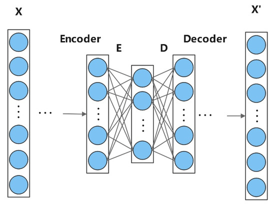
Figure 1.
Structure of DAE.
The core assumption of DAE for anomaly detection is that anomalous data are difficult to reconstruct accurately. Compared to normal data, anomalous data will encounter difficulties when reconstructed through low-dimensional representations, leading to significant deviations in the reconstructed results from the original inputs. In the decoding stage, the self-encoder seeks to minimize the reconstruction error by optimizing the reconstruction process to accurately restore the input data [20]. In this process, the self-encoder is able to effectively capture the characteristic patterns of normal data. The reconstruction error of anomalous data is usually large due to the pattern of the anomalous data not matching the normal data. Therefore, the reconstruction error is often used as a criterion to determine whether the data are abnormal or not. In DAE, the mean square error (MSE) is a commonly used loss function with the following mathematical expression:
where is the ith input vector, and is the corresponding reconstruction.
Although DAE can better extract data features, traditional autoencoder processing of time-series data has inherent limitations, mainly because it cannot effectively capture the temporal dependence between data and is sensitive to sequence length. This leads to the model having difficulty with learning the long-term dependency and data dynamic evolution laws. As a result, its feature-learning ability and generalization are more limited when dealing with complex time-series data.
2.2. Deep Autoencoding Gaussian Mixture Model (DAGMM)
DAGMM is an unsupervised anomaly method that combines reconstruction and density estimation. The model consists of a compression network and an evaluation network, and the compression network generates a low-dimensional representation of the data and reconstruction error using DAE and feeds it to the evaluation network, which further feeds it into a GMM [21]. The GMM learns the distribution pattern of the input features, giving the sample energy as an indicator of the anomaly, where the higher the sample energy, the more the data deviate from the normal data distribution. Instead of using decoupled two-stage training and the standard expectation–maximization (EM) algorithm [22], DAGMM jointly optimizes the parameters of both the deep autoencoder and the hybrid model in an end-to-end manner, utilizing a separate estimation network to facilitate parameter learning in the hybrid model. The joint optimization algorithm better balances automatic coding reconstruction, density estimation of potential representations, and regularization, which frees the encoder from the influence of local optimal solutions, further reduces the reconstruction error, and avoids the need for pre-training.
First, learn the low-dimensional feature using the deep self-coding network in the compression network and decode the low-dimensional feature to obtain the reconstruction x’, calculate the reconstruction error based on the reconstructed samples and the original samples to obtain the reconstruction error feature, and finally combine the low-dimensional feature and the reconstruction error feature to form a new feature Z. The specific processing flow of the compression network is shown in the following equation:
where is the encoding function; is the self-encoder parameter; is the decoding function; is the self-encoder parameter; and is the 2-parameter.
The evaluation network takes the low-dimensional features and reconstruction errors learned by the autoencoder as inputs. Its main function is to learn and output the parameters of the GMM, namely the posterior probability of each sample belonging to each Gaussian component, as well as the mean , covariance , and mixing coefficient of each Gaussian component. This process is realized by a multilayer perceptron : it nonlinearly transforms the features output from the self-encoder to obtain the GMM parameters needed to define and evaluate the “degree of abnormality” of each data point in a normal data distribution and outputs the negative log-likelihood of the GMM as an abnormality indicator. The negative log-likelihood of the GMM is output as the anomaly indicator. In short, the evaluation network combines the feature-learning capabilities of a self-encoder with probability density modeling to quantify the degree of anomalies in the data points.
At this point, the sample distribution of each distribution is determined by the given feature Z with the number of mixing components of feature K. The probabilistic output in GMM is the following:
The mixture probability of the kth component in the GMM is denoted as follows:
The mean of the kth component in the GMM is denoted as follows:
The covariance of the kth component in the GMM is expressed as follows:
The negative log-likelihood is calculated as follows:
where D is the feature dimension of feature .
3. Proposed Method
In this paper, we propose a novel anomaly detection method called the DAE-Transformer Gaussian Mixture Model (DTGMM). DTGMM aims to effectively identify anomalies in complex multivariate time-series data, overcoming the limitations of existing models in capturing intricate temporal dependencies between variables.
Multivariate time-series data consist of a sequence of multivariate vectors recorded chronologically, where denotes the observation at time t. Within the unsupervised learning paradigm for multivariate time-series anomaly detection, the model’s task is to grasp the inherent characteristics of a training dataset, without pre-labeled anomaly indicators. Following this learning process, the model then determines whether an observation at a future time point constitutes an anomaly. This is primarily achieved by quantitatively measuring the difference between training data T and new data . The proposed DTGMM is to take the difference between the distribution of untrained and normal samples as an abnormality score and compare this score with a threshold to determine whether it is abnormal or not.
3.1. DAE-Transformer-GMM (DTGMM)
3.1.1. Overall Architecture
The structure of the DTGMM proposed in this paper is shown in Figure 2. Compared with the traditional DAGMM, the DTGMM introduces a Transformer encoder specialized in capturing temporal dependencies at the feature extraction stage to capture the complex patterns of time-series data more comprehensively [23]. While DAGMM relies heavily on low-dimensional reconstructed features and reconstruction errors extracted by the self-encoder to learn potential representations of the data, DTGMM combines a DAE in parallel with a Transformer encoder that focuses on temporal feature learning to capture both structural anomalies and dynamic anomalies of the data in the time series.
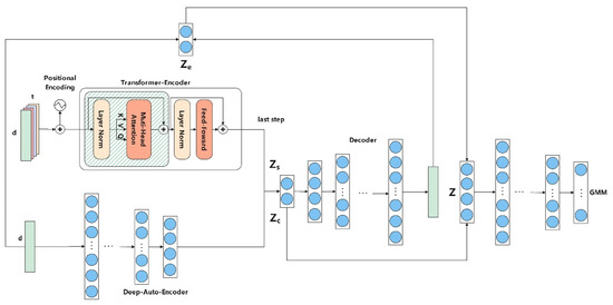
Figure 2.
DTGMM architecture.
DTGMM employs a two-way coding structure. The DAE is used to capture the static structure of the input data, generating the latent representation , while the Transformer encoder learns the time-dependent features through a self-attentive mechanism and outputs the locally dynamic representation. Decode and to obtain the reconstructed sample x’ and compute this to obtain the reconstructed error feature . The three are fused into a unified potential vector Z, which is richer and more informative than the single-source feature representation of DAGMM. The fused latent representations are not only used for data reconstruction to measure reconstruction errors but also as input to the GMM for probabilistic modeling. The GMM learns the latent distributions of the normal data, which are used in the inference phase to assess the degree of abnormality of new samples. Low likelihood values indicate their deviation from the normal pattern, indicative of abnormal data. The models are trained using end-to-end training.
3.1.2. Temporal Self-Attention Mechanism
In the Transformer encoder of DTGMM, in order to capture complex temporal dependencies in time-series data, we employ the temporal self-attention mechanism. Unlike DAGMM, which relies only on self-encoders to learn global or local feature representations, DTGMM is able to actively model the dependencies in the temporal dimension, thus capturing time-series anomalies more accurately.
Suppose the input to the Transformer encoder is , where t is the sequence length, and d is the number of features. In order to enhance the expressive power of the model, multi-head self-attention is used. For h heads, each head m computes its query (Q), key (K), and value (V) independently, and its final attention score is shown in the following equation:
where , , are weight matrices for the attention mechanism; Q, K, V are query vectors, key vectors, and value vectors; is the activation function; is the dimensionality of the key vectors; is the single-head output; is the weight matrix for the multi-headed attention; is the multi-headed output.
After obtaining the output of the self-attention, the temporal features can be obtained after residual joining and normalization, which are calculated as follows:
where is the layer normalization, and f is the fully connected layer.
With this design, DTGMM’s Transformer encoder is able to focus on capturing the temporal dynamics within the time-series data. This fine-grained temporal attention mechanism is the key to DTGMM’s superiority over DAGMM in handling temporal correlation anomalies in complex multivariate time series, as it is capable of identifying temporal pattern anomalies that are difficult to detect by global features alone (e.g., DAGMM).
3.1.3. DTGMM’s Latent Representation and Output
In DTGMM, we integrate information from the DAE and Transformer encoder to form a comprehensive latent representation and ultimately enable anomaly detection through the decoder and GMM. This contrasts with DAGMM, which only takes the reconstruction features and reconstruction errors of the self-encoder as inputs to the GMM, and DTGMM provides richer and more multimodal latent features.
As shown in Figure 2, DTGMM fuses latent variables from different encoders:
(Low-Dimensional Latent Representation): The output from the DAE can be obtained as in Equation (4), capturing the core content and structural information of the input data X. This part of the functionality is similar to the way DAGMM extracts core data features.
(Temporal Potential Representation): The output from the Transformer encoder is obtained from Equation (17), which mainly captures the temporal patterns and dynamic features of the input sequence. It enables the model to recognize timing anomalies that may be ignored by traditional reconstruction methods.
(Reconstruction Error Feature): The reconstruction error feature is computed as the difference between the original and reconstructed data vectors, which is calculated using Euclidean distance and cosine distance in this paper, as shown in Equations (18) and (19). This feature further enhances the learning ability of DTGMM on sample distribution features.
where is the second-order norm.
These latent representations, , , and , are spliced or otherwise fused (e.g., summed) to form the final composite latent vector Z. This multi-source feature fusion makes the latent space Z of the DTGMM more expressive and capable of encoding a more comprehensive and varied range of “normal” patterns. The fused potential vector Z is then fed into an evaluation network. The decoder is a network of multiple fully connected layers whose task is to output the GMM parameters as in Equations (8)–(11). The GMM models the distribution of normal data over the latent space Z. The ability of the GMM to represent complex multi-peak distributions allows it to capture multiple “normal” patterns. In the inference phase, for a new input data X′, it undergoes the same encoding process to obtain the potential vector Z′. The GMM then computes the value of the probability density function of Z′ under its learned normal distribution. If Z′ falls into the low-density region of the GMM distribution (i.e., its probability value is small), it indicates that X′ deviates from the normal pattern; conversely, if Z′ falls into the high-density region, it indicates that X′ is normal. The negative log-likelihood (NLL) is usually used as the anomaly score [24], which can be calculated as in Equation (12). The higher the NLL, the higher the likelihood that the data point is an anomaly. Compared to DAGMM, the potential space Z of GMM modeling for DTGMM contains more timing and global context information from the Transformer. This means that DTGMM’s GMM is able to capture richer and finer distributions of normal data, resulting in greater robustness and accuracy in identifying anomalies, especially in time-series data.
3.1.4. Loss Function
The DTGMM constructed in this study employs a combined loss function designed to optimize both the reconstruction quality and the latent spatial distribution modeling. The overall loss function includes the reconstruction error and GMM likelihood terms as well as the matrix singularity penalty term as shown in the following equation:
where and are the weights of the sample energy and canonical terms, d denotes the number of dimensions in the low-dimensional space, and denotes the j-th diagonal element of the covariance matrix of the Gaussian component k.
The design of this loss function, the reconstruction loss, is intended to force the encoder to learn a compact representation that captures the structure and content of the original data and enables the decoder to accurately reconstruct the normal data. By minimizing the reconstruction error, the model is able to extract a compact representation from the training data that accurately reflects the structure of the original time-series data; the GMM likelihood loss is intended to optimize the parameters of the GMM so that it can better fit the distribution of normal data in the latent space Z; the matrix singular value penalty is intended to avoid matrix irreducibility.
3.2. Anomaly Detection Process
The process of assessing the health status of key equipment of coal power units based on DTGMM can be divided into two parts: offline training and online assessment, as shown in Figure 3. The two parts include the acquisition of multivariate time series, data preprocessing, and normalization, and the processed health data will be input into the DTGMM to calculate the abnormal scores and then set the thresholds according to the normal samples. Then, the test set will be input into the model to judge the thresholds according to the device status.
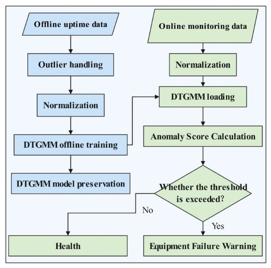
Figure 3.
Flowchart for equipment health assessment.
3.2.1. Data Preprocessing
The data used for modeling in this study are derived from actual power plant operations. In the process of power plant data collection, sensor failures, communication interference, or sudden equipment conditions may lead to outliers and missing values in the raw data. Directly using such data for energy efficiency analysis or fault diagnosis will introduce significant bias, which will seriously affect the model performance [25]. Given that the training data contain only samples under normal working conditions, since the training data use sample data under normal working conditions, this section uses the sliding window outlier coefficient method for outlier processing, which calculates the data outlier distance and outlier coefficient through a dynamic window to ensure that there is no outlier in the normal data, setting the sliding window to be w, and the original data to be , and then the formula is as follows:
where , are the mean and variance, and is the outlier coefficient, which is usually considered to be greater than 3 for outlier points.
Take the establishment of a power plant superheater equipment condition monitoring model as an example, in which the abnormal values of the turbine water level in the training data are handled as shown in Figure 4. The abnormal value detection helps to identify atypical behaviors in the operation process and prevents them from interfering with the model’s learning law.
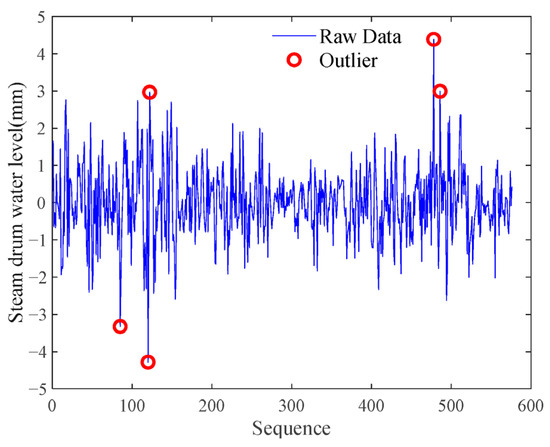
Figure 4.
Abnormal treatment of vapor packet water level.
For the missing values, the time-series linear interpolation method is used to fill in the missing values based on the linear trend of the data in the neighboring time periods, which can not only retain the time sequence continuity of the operation of the equipment but also avoid the computational burden of the complex model, and its calculation formula is as follows:
where t is the corresponding time, and is the variable at the same time.
Due to the different scales of the selected parameters, the huge difference in values between different parameters needs to be normalized for these parameter values, and the normalization formula is as follows:
3.2.2. Model Construction
After preprocessing the normal operation data, the features are fed into the DTGMM for training; the DTGMM can be divided into a compression network and an evaluation network, where the compression network includes an encoder as well as a decoder, and the hyperparameters to be determined in the encoder are the number of self-attention headers in the Transformer, the number of units of the fully-connected layers of the numKeyChannels as well as the activation function in DAE, the number of fully connected layers, and the number of cells and activation functions in DAE; the hyperparameters to be determined in the decoder are the number of fully connected layers, the number of cells, and the activation function; the hyperparameters to be determined in the evaluation network (GMM) are the number of fully connected layers, the number of cells, and the activation function. The last thing that needs to be determined is the weight of the loss function. In this study, the model hyperparameters were determined through multiple experiments. The weights in the loss function were optimized using a Bayesian optimization algorithm, with the search range for λ1 set to [0,1] and for λ2 set to [0,0.01]. The optimization was performed over 20 iterations. All the above processes were implemented using MATLAB R2023b software. The number of training epochs was set to 500, and the response time for a single inference was 0.03 s, which meets the requirements for real-time early warning deployment. Taking the superheater condition monitoring model of a certain power plant as an example, the specific hyperparameter settings are shown in Table 1.

Table 1.
Hyperparameter settings for DTGMM models.
3.2.3. Equipment Health Assessment and Early Warning of Failures
Taking the boiler superheater of a power plant as an example, the operating data of the boiler superheater in a healthy state is used as a training set to train the DTGMM, obtain optimal network parameters, and complete the local storage of the model. With the accumulation of historical offline monitoring data, the health assessment model can be retrained and parameters updated periodically to adapt to the long-term changes in the operating state of the equipment. The critical operational data of the superheater collected online in real time will be fed as input to the trained DTGMM for health assessment after preprocessing such as normalization and sliding window slicing.
There are multiple dynamic disturbances during boiler operation, such as load fluctuation, combustion adjustment, energy-saving optimization operation, etc., which cause the superheater data samples to show non-stationary characteristics. Even in the absence of obvious faults, the model’s health indicator outputs may still exhibit fluctuations, so the output results of the DTGMM are usually in a state of dynamic equilibrium. To enhance the early warning robustness of the model, this paper introduces a sliding average mechanism at the output end of the abnormality scores and performs time smoothing on the health scores generated by the GMM to reduce the interference of the high-frequency noise in the model reconstruction error on the results. Ultimately, a kernel density estimation-based approach is used to model the health score distribution, and the health score at 98% cumulative probability is used as a failure warning threshold for identifying potential operational anomalies or performance degradation trends.
3.2.4. Model Evaluation Metrics
Given that the field data used in this study lack explicit fault labels and the research focuses on early warning capabilities, the following three performance metrics are adopted:
Detection Delay: This metric evaluates the model’s ability to provide early warnings. It is calculated as follows:
where is the time at which the model issues a warning, and is the actual onset time of the event.
False Negative Rate (FNR): This metric assesses the miss rate of anomaly detection models, defined as the proportion of actual positive samples incorrectly classified as normal among all actual positive samples. It is calculated as follows:
where (false negatives) represents samples that are actually anomalous but predicted as normal, and (true positives) represents samples that are correctly predicted as anomalous.
Early Warning False Negative Rate (EWFNR): This metric evaluates the miss rate after the model issues a warning, calculated as follows:
where and denote the false negatives and true positives, respectively, under the condition that the model has issued a warning.
4. Example Analysis
4.1. Boiler Superheater Condition Monitoring
Taking the low-temperature superheater of the boiler of a power plant as the object of study, the leakage alarm occurred in this plant on 8 July, but there was no significant change in the operating parameters, and the boiler was shut down on 13 July, and the issue was later confirmed to be a leakage of the low-temperature superheater piping. For this reason, we selected the sample data from 3 July to 25 July 2023, considering that there is no direct measurement point for the cryogenic superheater piping. From the perspective of boiler operation mechanisms, relevant parameters that reflect the thermal boundaries and operating conditions of the low-temperature superheater were selected as the feature set, as shown in Table 2. The feedwater flow rate and main steam flow rate characterize the overall flow conditions of the boiler’s water–steam system, while the main steam temperature, pressure, and load represent the current operating status of the boiler. The primary desuperheating water flow and the steam temperatures before and after the attemperator directly affect the heat distribution in the subsequent superheaters. The outlet steam temperature of the rear screen superheater and the flue gas temperature at the low-temperature superheater inlet together describe the thermal state at the inlet and outlet of the low-temperature superheater. Additionally, the flue gas oxygen content reflects the combustion condition and flue gas quality, indirectly affecting the heat transfer performance of the superheater. These parameters comprehensively consider heat sources, fluid flow, and load conditions, thus providing a solid mechanistic basis for anomaly detection. The data used for evaluation are sampled at intervals of five minutes. The sliding window is set to 10.
Table 2.
DAGMM input variables.
4.1.1. Anomaly Detection
This study validates the proposed model using a real-world fault case from a coal-fired power plant. On 8 July 2023, at around 19:00, a leak alarm was triggered at Boiler #1, Tube #19, indicating a potential tube leak. However, no significant change was observed in the operational parameters at that time, and the unit appeared to be operating normally. On the morning of 9 July, after opening the upper manhole of the low-temperature superheater’s fixed end, maintenance personnel confirmed a leak in the low-temperature superheater pipeline. The unit was eventually shut down for maintenance on 13 July. Given that the leak issue had been resolved, data from 22 July to 25 July were selected as the training set, while data from 2 July to 14 July were used as the test set.
To verify the effectiveness of the proposed method, three baseline models were selected for comparison: the traditional DAGMM, the TGMM, and the widely adopted long short-term memory variational autoencoder (LSTM-VAE) model. Corresponding performance metrics were calculated, as shown in Table 3.
Table 3.
Comparison of model performance.
DTGMM demonstrates superior performance in early warning tasks, with a detection delay of −90 h, providing ample lead time before the actual fault occurred—outperforming all baseline models. This advantage stems from DTGMM’s integration of dynamic temporal modeling with a Gaussian mixture model, allowing it to capture complex temporal patterns and identify potential anomalies in advance. Moreover, DTGMM achieves the lowest EWFNR, reducing the weighted missed detection rate by 70% compared to TGMM, indicating its strong reliability in high-risk scenarios. The FNR is also relatively low at 0.0913, second only to DAGMM.
In comparison, DAGMM achieves the lowest FNR (0.0547), likely due to its deep autoencoder’s enhanced feature extraction capability. However, its detection delay is shorter than DTGMM, which could limit its usefulness in early warning contexts. TGMM and LSTM-AE, on the other hand, perform poorly in both FNR and EWFNR, particularly LSTM-VAE, which exhibits the highest missed detection rate (FNR = 0.7251). This may be due to LSTM-VAE’s limited ability to model subtle anomaly patterns or overfitting to normal data due to class imbalance.
As shown in Figure 5 (where the red dashed line denotes the threshold and the blue curve represents the variation trend of the anomaly score), the anomaly scores from the four models demonstrate significant differences. DTGMM successfully detected signals exceeding the preset threshold as early as the early morning of 5 July, offering a nearly three-day lead time before the confirmed fault. Throughout the normal operation period, it produced minimal false alarms, with stable curve behavior and clear warning points, highlighting its strong anomaly capture capability and practical value.
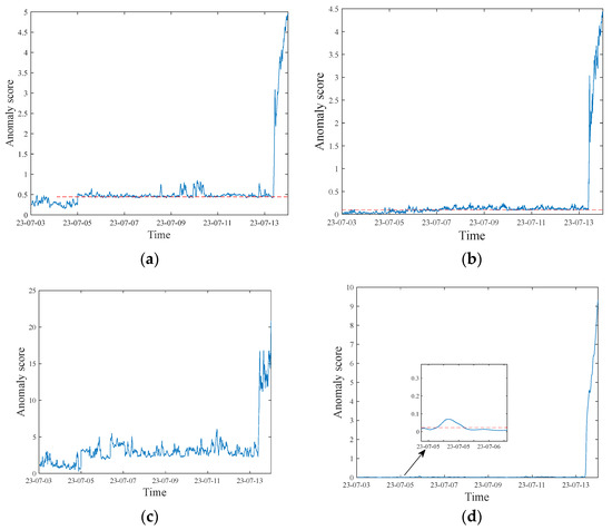
Figure 5.
Superheater anomaly detection results under different models: (a) DTGMM; (b) DAGMM; (c) Transformer-GMM; (d) LSTM-VAE.
TGMM also showed decent performance, issuing its first warning signal on 5 July as well, though slightly later than DTGMM. However, its score curve fluctuates heavily throughout the monitoring period, resulting in a high false alarm rate. This can cause alarm fatigue and reduce trust in the model’s predictions, thus lowering its practical applicability. In contrast, the DAGMM model issued its first threshold-crossing signal on 7 July, just one day before the confirmed fault. Although it still managed to issue a timely warning, it showed several false positives during the early stages of operation, triggered by minor fluctuations. While not overly disruptive, this behavior suggests that additional diagnostic support might be required for reliable deployment.
Overall, DTGMM stands out as the only model that effectively balances early warning, low false alarm rate, and high stability. Its architecture integrates feature extraction, temporal modeling, and probabilistic decision making into a cohesive framework. This results in strong global modeling capacity and consistent anomaly discrimination. It not only captures subtle trend shifts but also suppresses interference from local noise, enabling early alerts well before the actual failure while maintaining a low false positive rate. In contrast, while TGMM and LSTM-VAE offer some early detection capabilities, their architectures lack robust feature representation, leading to frequent false alarms. DAGMM, limited by weak temporal modeling capacity, struggles to detect subtle anomalies in complex time series, resulting in delayed warnings and higher sensitivity to minor disturbances, reducing its overall stability.
4.1.2. Feature Analysis
To enhance the interpretability of the model, this study introduces the SHAP (Shapley additive explanations) method to analyze the feature contribution of the constructed superheater anomaly detection model. SHAP values measure the marginal contribution of each feature to the model’s predictive output, reflecting its impact on the anomaly score.
Figure 6 shows a bar chart of the average SHAP values corresponding to the 11 input features. The analysis results indicate significant differences in the model’s sensitivity to different input variables.
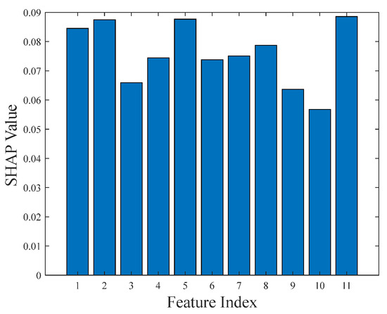
Figure 6.
SHAP values of different features.
Main steam flow, load, and flue gas temperature at the low-temperature superheater inlet exhibit the highest average SHAP values, indicating that the model relies heavily on these variables when determining anomalies. Main steam flow and load are core operational parameters of the thermal system, often directly reflecting changes in system demand, while flue gas temperature is directly related to the thermal state of the heat exchanger. Therefore, these three collectively constitute key indicators for identifying abnormal conditions in the superheater.
In contrast, main steam temperature, flue gas oxygen content, and rear screen superheater outlet steam temperature have the lowest SHAP values (approximately 0.06), suggesting that the model depends less on these features. Although they are also physically related to the thermal state of the system, their low weights may be due to smaller changes during anomalies or redundancy with other variables.
The remaining features, such as primary desuperheating water flow and main steam pressure, exhibit intermediate SHAP values, indicating that while they are not primary drivers, they still play a supplementary role in the model.
In conclusion, the SHAP results exhibit strong consistency with physical mechanisms, validating the model’s effectiveness in focusing on critical operational parameters. Since the model detects anomalies by learning the high-dimensional distribution of input features, all features maintain relatively high influence levels. Additionally, SHAP analysis provides operators with prioritized monitoring targets.
4.2. Validation of Other Equipment
In order to verify the generality of the model, DTGMM was used to model the turbine bearing condition of a power plant, where abnormal four-tile vibration was found at 12:05 on 7 September 2023, and a large turbine vibration trip event occurred at 12:35 on Unit 1. It was determined that the reason was the temperature difference between the low-pressure cylinder block and the exhaust steam, and the low-pressure cylinder block was gradually deformed; meanwhile, the vacuum of the unit increased, and there was air leakage in the shaft seal, which firstly caused the steam seal of the axle end to be stored in a certain amount of deformation (the clearance between the axle and the shaft seal was 0.5 mm), and the clearance between the axle and the shaft seal became smaller, resulting in the dynamic and static friction of the shaft seal at the four tiles of the #1 turbine and the vibration of the axle tiles with the large value of jumping caused by the turbine.
This study selects the running data from 25 August to 7 September, with the running data from 25 August to 2 September as the training set and the running data from 3 September to 7 September as the test set. The corresponding input variables are presented in Table 4, and the test results are shown in Figure 7.
Table 4.
DAGMM input variables of the shaft.
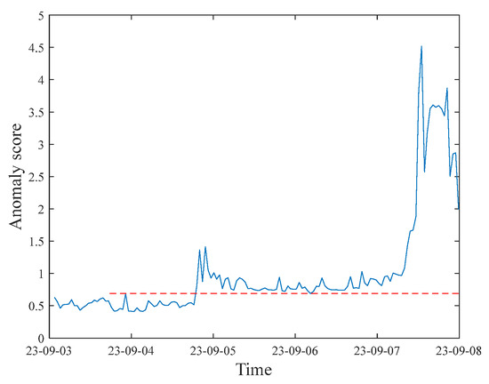
Figure 7.
Abnormal detection of turbine bearing status based on DTGMM.
In the test set, the first time the anomaly score exceeded the threshold occurred at 19:10 on 4 September, about three days earlier than the actual discovery of the anomaly, and then the indicator continued to be in the over-threshold state, indicating that the equipment has been abnormal and continues to deteriorate, which needs to draw the attention of the operation personnel and take measures in a timely manner. In particular, on 7 September, the day of the failure, there was a significant jump in the health indicators, indicating that the equipment was close to the edge of failure, which ultimately led to the actual tripping accident at the site, further verifying the accuracy and practicability of the model in the early warning of failures and trend judgments.
5. Conclusions
In this study, a deep learning anomaly detection model (DTGMM) based on DAE, Transformer, and GMM is successfully constructed and validated, aiming to enhance the condition monitoring and early warning capability of key equipment in coal-fired power plants. The model extracts the static features of the data through DAE and captures the timing dependencies using the Transformer encoder, and finally the GMM learns the data distribution of the normal operating conditions to identify the anomalies.
The validity and superiority of the model are verified by analyzing the actual operation data of boiler superheaters and turbine bearings in a power plant in an arithmetic example. In the case of the superheater leak, DTGMM was able to detect the anomaly earlier than the traditional DAGMM and Transformer-GMM models, issuing an early warning nearly three days ahead of time and performing more consistently and with fewer false alarms during normal operation. In the case of turbine bearing vibration anomalies, the model was also successful in detecting the anomalous signals about three days before the actual occurrence of the failure and was able to track the trend of continuous deterioration of the equipment condition, proving the versatility of the model and the value of early warning in practical applications.
Taken together, DTGMM effectively solves the limitations of traditional methods in dealing with complex time-series data by integrating the advantages of multiple networks structures, realizes the keen capture of weak abnormal signals of the equipment, and excels in the advance, accuracy, and stability of early warning. The research results are of great significance for guaranteeing the safety of the unit and realizing intelligent overhaul and maintenance. Considering the limitations of the actual fault dataset, the impact on the model itself is significant. Future work could explore methods such as generating synthetic fault samples to further enhance the model’s generalization ability.
Author Contributions
Conceptualization, S.W., C.Z., X.G. and L.S.; methodology, S.W., X.L., X.G. and L.S.; software, X.L. and X.C.; validation, X.L. and S.W.; formal analysis, S.W.; investigation, S.W.; resources, X.N.; data curation, X.N. and X.G.; writing—original draft preparation, S.W.; writing—review and editing, X.C.; visualization, C.Z.; supervision, L.S.; project administration, S.W. and L.S.; funding acquisition, S.W. and L.S. All authors have read and agreed to the published version of the manuscript.
Funding
This research was funded by the National Natural Science Foundation of China (NSFC) under grant 52276003, Grant of Guoneng Nanjing Electric Power Test & Research Limited, grant number DY2024Y02, and the Science and Technology Innovation Project of China Energy Investment Corporation, grant number GJNY-23-68 and the Fundamental Research Funds for the Central Universities: 2242025K30015, Southeast University.
Data Availability Statement
The datasets presented in this article are not readily available because the data used in this article are confidential. Requests to access the datasets should be directed to corresponding author.
Conflicts of Interest
Authors Shuchong Wang, Changxiang Zhao, Xingchen Liu, Xianghong Ni, and Xu Chen were employed by the company Guoneng Nanjing Electric Power Test & Research Limited, China. Author Xinglong Gao was employed by the company China Energy Changzhou Secondary Power Generation CO., Ltd. The remaining authors declare that the research was conducted in the absence of any commercial or financial relationships that could be construed as a potential conflict of interest.
References
- Fausing Olesen, J.; Shaker, H.R. Predictive maintenance for pump systems and thermal power plants: State-of-the-art review, trends and challenges. Sensors 2020, 20, 2425. [Google Scholar] [CrossRef]
- Velayutham, P.; Ismail, F.B. A review on power plant maintenance and operational performance. MATEC Web Conf. 2018, 225, 05003. [Google Scholar] [CrossRef]
- Wang, P.; Tian, X.; Sun, K.; Huang, Y.; Wang, Z.; Sun, L. Power System Reliability Assessment Considering Coal-Fired Unit Peaking Characteristics. Algorithms 2025, 18, 197. [Google Scholar] [CrossRef]
- Choi, H.; Kim, C.W.; Kwon, D. Data-driven fault diagnosis based on coal-fired power plant operating data. J. Mech. Sci. Technol. 2020, 34, 3931–3936. [Google Scholar] [CrossRef]
- Miao, J.; Tao, H.; Xie, H.; Sun, J.; Cao, J. Reconstruction-based anomaly detection for multivariate time series using contrastive generative adversarial networks. Inf. Process. Manag. 2024, 61, 103569. [Google Scholar] [CrossRef]
- Agrawal, V.; Panigrahi, B.K.; Subbarao, P.M.V. Review of control and fault diagnosis methods applied to coal mills. J. Process Control 2015, 32, 138–153. [Google Scholar] [CrossRef]
- Qiu, J.; Zhang, X.; Wang, T.; Hou, H.; Wang, S.; Yang, T. A GNN-Based False Data Detection Scheme for Smart Grids. Algorithms 2025, 18, 166. [Google Scholar] [CrossRef]
- Nachman, B.; Shih, D. Anomaly detection with density estimation. Phys. Rev. D 2020, 101, 075042. [Google Scholar] [CrossRef]
- Hu, W.; Gao, J.; Li, B.; Wu, O.; Du, J.; Maybank, S. Anomaly detection using local kernel density estimation and context-based regression. IEEE Trans. Knowl. Data Eng. 2018, 32, 218–233. [Google Scholar] [CrossRef]
- Dang, T.T.; Ngan, H.Y.T.; Liu, W. Distance-based k-nearest neighbors outlier detection method in large-scale traffic data. In Proceedings of the 2015 IEEE International Conference on Digital Signal Processing (DSP), Singapore, 21–24 July 2015; pp. 507–510. [Google Scholar]
- Choi, Y.; Lim, H.; Choi, H.; Kim, I.J. Gan-based anomaly detection and localization of multivariate time series data for power plant. In Proceedings of the 2020 IEEE International Conference on Big Data and Smart Computing (BigComp), Busan, Korea, 19–22 February 2020; pp. 71–74. [Google Scholar]
- Hu, D.; Zhang, C.; Yang, T.; Chen, G. Anomaly detection of power plant equipment using long short-term memory based autoencoder neural network. Sensors 2020, 20, 6164. [Google Scholar] [CrossRef]
- Fahmi, A.T.W.K.; Kashyzadeh, K.R.; Ghorbani, S. Fault detection in the gas turbine of the Kirkuk power plant: An anomaly detection approach using DLSTM-Autoencoder. Eng. Fail. Anal. 2024, 160, 108213. [Google Scholar] [CrossRef]
- Li, Y.; Jiang, W.; Zhang, G.; Shu, L. Wind turbine fault diagnosis based on transfer learning and convolutional autoencoder with small-scale data. Renew. Energy 2021, 171, 103–115. [Google Scholar] [CrossRef]
- He, Q.; Li, Y.; Jiang, G.; Su, N.; Xie, P.; Wu, X. Health assessment of wind turbine gearboxes based on conditional convolutional self-coding Gaussian mixture models. Acta Energiae Solaris Sin. 2023, 44, 214–220. [Google Scholar]
- Hu, D.; Zhang, C.; Yang, T.; Fang, Q. A deep autoencoder with structured latent space for process monitoring and anomaly detection in coal-fired power units. Reliab. Eng. Syst. Saf. 2025, 261, 111060. [Google Scholar] [CrossRef]
- Li, X.; Huang, T.; Cheng, K.; Qiu, Z.; Sichao, T. Research on anomaly detection method of nuclear power plant operation state based on unsupervised deep generative model. Ann. Nucl. Energy 2022, 167, 108785. [Google Scholar] [CrossRef]
- Mienye, I.D.; Swart, T.G. Deep autoencoder neural networks: A comprehensive review and new perspectives. Arch. Comput. Methods Eng. 2025, 1–20. [Google Scholar] [CrossRef]
- Mejri, N.; Lopez-Fuentes, L.; Roy, K.; Chernakov, P.; Ghorbel, E.; Aouada, D. Unsupervised anomaly detection in time-series: An extensive evaluation and analysis of state-of-the-art methods. Expert Syst. Appl. 2024, 256, 124922. [Google Scholar] [CrossRef]
- Zhou, C.; Paffenroth, R.C. Anomaly detection with robust deep autoencoders. In Proceedings of the 23rd ACM SIGKDD International Conference on Knowledge Discovery and Data Mining, Halifax, NS, Canada, 13–17 August 2017; pp. 665–674. [Google Scholar]
- Zong, B.; Song, Q.; Min, M.R.; Cheng, W.; Lumezanu, C.; Cho, D.; Chen, H. Deep autoencoding gaussian mixture model for unsupervised anomaly detection. In Proceedings of the International Conference on Learning Representations, Vancouver, BC, Canada, 30 April–3 May 2018. [Google Scholar]
- Yang, X.; Li, Y.; Zhao, Y.; Li, Y.; Hao, G.; Wang, Y. Gaussian mixture model uncertainty modeling for power systems considering mutual assistance of latent variables. IEEE Trans. Sustain. Energy 2024, 16, 1483–1486. [Google Scholar] [CrossRef]
- Habeb, M.H.; Salama, M.; Elrefaei, L.A. Enhancing video anomaly detection using a transformer spatiotemporal attention unsupervised framework for large datasets. Algorithms 2024, 17, 286. [Google Scholar] [CrossRef]
- Chen, Y.; Ashizawa, N.; Yeo, C.K.; Yanai, N.; Yean, S. Multi-scale self-organizing map assisted deep autoencoding Gaussian mixture model for unsupervised intrusion detection. Knowl -Based Syst. 2021, 224, 107086. [Google Scholar] [CrossRef]
- Lin, Z.; Wang, H.; Li, S. Pavement anomaly detection based on transformer and self-supervised learning. Autom. Constr. 2022, 143, 104544. [Google Scholar] [CrossRef]
Disclaimer/Publisher’s Note: The statements, opinions and data contained in all publications are solely those of the individual author(s) and contributor(s) and not of MDPI and/or the editor(s). MDPI and/or the editor(s) disclaim responsibility for any injury to people or property resulting from any ideas, methods, instructions or products referred to in the content. |
© 2025 by the authors. Licensee MDPI, Basel, Switzerland. This article is an open access article distributed under the terms and conditions of the Creative Commons Attribution (CC BY) license (https://creativecommons.org/licenses/by/4.0/).