Adaptive Real-Time Planning of Trailer Assignments in High-Throughput Cross-Docking Terminals

Abstract

Cross-docking has emerged as a critical logistics strategy to reduce lead times, lower inventory levels, and enhance supply chain responsiveness. However, in high-throughput terminals, efficient coordination of inbound and outbound trailers remains a complex task, especially under uncertain and dynamically changing conditions. We propose a practical framework that helps logistics terminals assign trailers to docks in real time. It links live sensor data with a mathematical optimization model, so that the system can quickly adjust trailer plans when traffic or workload changes. Real-time data from IoT sensors, GPS, and operational records are preprocessed, enriched with predictive analytics, and used as input for a Mixed-Integer Linear Programming (MILP) model solved in rolling horizons. This enables the continuous reallocation of inbound and outbound trailers, ensuring synchronized flows and balanced dock utilization. Numerical experiments compare the adaptive approach with conventional first-come-first-served scheduling. Results show that average inbound dock utilization improves from 68% to 71%, while the share of periods with full utilization increases from 33.3% to 41.4%. Outbound utilization also rises from 57% to 62%. Moreover, trailer delays are significantly reduced, and the overall makespan shortens from 45 to 40 time slots. These findings confirm that adaptive, real-time trailer assignment can enhance efficiency, reliability, and resilience in cross-docking operations. The proposed framework thus bridges the gap between static optimization models and the operational requirements of modern, high-throughput logistics hubs.

1. Introduction

Cross-docking has become a widely adopted logistics practice to reduce lead times, minimize inventory, and increase supply chain responsiveness. By transferring goods directly from inbound to outbound vehicles with little or no storage, cross-docking offers significant cost and service benefits compared to conventional warehousing. At the same time, this mode of operation creates considerable complexity, especially in high-throughput environments where numerous trucks must be coordinated under uncertain and rapidly changing conditions. Efficient trailer assignment and dock planning are therefore central to ensuring that cross-docking terminals achieve their intended performance.

The academic literature has extensively examined these challenges. Foundational studies established models for truck scheduling and dock assignment, providing key insights into how inbound and outbound flows can be synchronized (Boysen et al., 2010 [1]; Cota et al., 2016 [2]). Later research began to account for uncertainty and sector-specific requirements, such as stochastic arrivals or perishables handling, highlighting the importance of robust and responsive solutions (Gallo et al., 2022 [3]; Zheng et al., 2021 [4]). Other contributions have emphasized that terminal operations cannot be viewed in isolation but must be coordinated with broader distribution networks, showing how inefficiencies at the dock propagate into the wider supply chain (Coindreau et al., 2021 [5]; Buijs et al., 2016 [6]).

In parallel, new technologies are starting to reshape how cross-docking can be managed. Blockchain and IoT-based solutions, for example, have been proposed to improve transparency, coordination, and risk management across terminal operations (Liu & Li, 2023 [7]; Pan et al., 2021 [8]). While promising, such approaches have so far been applied mainly to information sharing or monitoring, rather than to the adaptive reallocation of resources inside high-volume facilities.

Previous research has mostly focused on planning before execution. However, in real terminals, trailer arrivals and dock workloads change from minute to minute. Our study focuses on how to react to these fluctuations instead of relying on fixed plans. What is missing is an operational framework that combines the insights of scheduling models, network integration, and digital technologies into adaptive, real-time trailer assignment strategies.

This paper responds to that gap by proposing an approach for adaptive real-time planning of trailer assignments in high-throughput cross-docking terminals. The framework builds on established scheduling principles but extends them into a dynamic control layer, capable of reacting to live system states and rebalancing workloads accordingly. In this way, it bridges the divide between static optimization and operational reality, enabling cross-docking terminals to maintain both efficiency and resilience under volatile conditions.

The remainder of this article is structured as follows: Section 2 presents a comprehensive literature review on design and operation of cross-docking. Section 3 introduces the conceptual model framework and the mathematical model of adaptive real-time planning of trailer assignments, while Section 4 details the numerical results. Section 5 discusses the implications for industrial practice, followed by concluding remarks.

2. Literature Review

We first summarize the main studies and publication trends. Next, we review their key findings and limitations. Finally, we highlight specific open problems that motivated our own model.

2.1. Descriptive Analysis

As part of the systematic literature review, we followed a structured procedure. The process included several steps: defining the research questions, selecting relevant sources from Scopus, refining the article list through screening and topic identification, analyzing the contributions, summarizing their key findings, and identifying remaining research gaps and bottlenecks.

To conduct the database search, we applied the keyword “cross-docking” but we added some other logistics related words with an OR operator exclude results related to the following topics: computational biology, bioinformatics; medicinal chemistry & drug discovery; structural biology; pharmacology; chemoinformatics; neuroscience; cancer research; virology & microbiology. The initial search resulted in 600 articles. We then refined the selection by applying the following filters: (TITLE-ABS-KEY (cross-docking) AND TITLE-ABS-KEY (warehouse) OR TITLE-ABS-KEY (logistics) OR TITLE-ABS-KEY (terminal) OR TITLE-ABS-KEY (transportation) OR TITLE-ABS-KEY (loading)) AND (LIMIT-TO (DOCTYPE, “ar”) OR LIMIT-TO (DOCTYPE, “cp”) OR LIMIT-TO (DOCTYPE, “ch”)) AND (LIMIT-TO (LANGUAGE, “English”)). Only peer-reviewed journal articles written in English were retained, resulting in a final dataset of 540 articles. The search was carried out in September 2025; therefore, additional relevant publications may have appeared since that time.

The selected articles can be classified by research area. Figure 1 shows the classification of these 540 articles considering ten subject areas. This classification shows that the majority are engineering and computer science, whilst environmental science and energy highlight the increased sustainability aspects of design and operation of cross-docking terminals and mathematics focuses on the optimization of cross-docking-based supply chain solutions.

As Figure 2 illustrates, research on cross-docking solutions has been continuously and intensively conducted over the past 10 years.

As Figure 3 depicts, most of the articles were published in journals with optimization topics, but a significant number of the papers were accepted for publication in journals focusing on industrial engineering, operation research, production research, expert systems and machine learning, production economics, logistics management, and transportation.

We have analyzed the distribution of articles in the following categories: scheduling, trucks, integer programming, logistics, supply chain, optimization, warehouses, vehicle routing, supply chain management, heuristic optimization, costs, sales, unloading. Figure 4 depicts the distribution of the categories. As the categories show, the design and operation of cross-docking-based logistics and supply chain solutions is based on multidisciplinary, where scheduling, optimization, transportation technology, finance, logistics operations are integrated.

In the following step, the 540 articles were reduced after reading them. We excluded articles whose topic did not fit our interest and did not address the optimization of cross-docking terminals.

2.2. Content Analysis

To guide the content analysis, the literature on cross-docking is organized into five main areas: (1) truck scheduling and operational planning, (2) vehicle routing and cross-docking integration, (3) network design and facility location, (4) sustainability, digitalization, and new technologies, and (5) strategic and managerial aspects. This structure allows for a focused synthesis of prior work and a clear identification of research gaps relevant to adaptive real-time trailer assignment in high-throughput cross-docking terminals.

2.2.1. Truck Scheduling and Operational Planning in Cross-Docking Terminals

Truck scheduling and operational planning are core challenges in cross-docking research, as they directly determine terminal throughput, resource utilization, and service reliability. Early contributions recognized truck scheduling as a combinatorial optimization problem with significant computational complexity. Boysen et al. (2010) [9] formulated the simultaneous scheduling of inbound and outbound trucks at cross-docking terminals, and focused on zero-inventory cross-docks, stressing the difficulty of balancing synchronization with strict time constraints.

Research in the 2010s expanded to cover information availability and robustness. Larbi et al. (2011) [10] analyzed scheduling performance under full, partial, and no information on arrivals, whereas Alpan et al. (2011) [11] applied bounded dynamic programming to generate efficient schedules. Vahdani and Zandieh (2010) [12] developed robust meta-heuristics capable of coping with stochastic disruptions, and Choy et al. (2012) [13] examined job assignment problems in space-constrained facilities, where docking capacity severely limits flexibility.

Later studies emphasized flow shop and heuristic formulations. Fonseca et al. (2019) [14] applied Lagrangian relaxation in hybrid flow-shop scheduling, while Nogueira et al. (2020) [15] extended the problem to parallel-machine environments, showing improved scalability. Ardakani et al. (2020) [16] introduced sequencing approaches that consider repeat truck holding patterns, and Pan et al. (2021) [17] proposed repeated loading schedules to reduce deterioration in perishable products. Zheng et al. (2021) [4] focused on cold-chain truck scheduling, introducing heuristics for handling temperature-differentiated flows.

Industry-specific applications also highlight the relevance of truck scheduling. Mejía et al. (2023) [18] studied the Colombian flower export sector, proposing queue management and scheduling to mitigate congestion at airports. Luo et al. (2019) [19] addressed synchronized scheduling between make-to-order plants and cross-docking warehouses. Chargui et al. (2019) [20] incorporated energy consumption into truck scheduling in rail-road physical internet hubs. Braglia et al. (2019) [21] emphasized visual planning approaches, inspired by lean management, to improve daily scheduling transparency.

Recent methodological progress includes stochastic and multi-objective formulations. Gallo et al. (2022) [3] introduced a stochastic genetic algorithm to handle uncertain arrivals, significantly reducing penalty costs. Chargui et al. (2022) [22] developed MILP and meta-heuristics for multi-door terminals with multiple storage zones, while Taghizadeh et al. (2022) [23] proposed a bi-objective model balancing makespan and handling costs. He and Prabhu (2022) [24] extended the scope to AGV-based systems, applying analytical models to dimension fleets and predict service rates. Kravchuk & Kravchuk (2024) [25] focuses on simulation-based optimization of truck scheduling and dock operations.

Other lines of research focus on optimization techniques for multi-door and multi-objective problems. Wisittipanich and Hengmeechai (2015) [26] used differential evolution for door assignment and truck scheduling, while Mohtashami (2015) [27] and Kim and Joo (2015) [28] developed heuristics for multi-door truck scheduling with temporary storage. Cota et al. (2016) [2] proposed a time-indexed formulation and heuristic for multi-dock problems, while Noh et al. (2025) [29] advanced inbound scheduling with real-time dynamic rescheduling.

Table 1. Overview of Key Studies on Truck Scheduling and Operational Planning in Cross-Docking Terminals.

Theme	Focus	Approach
Foundational models [9]	Truck scheduling, zero-inventory	Exact + heuristics
Uncertainty & robustness [3,10,11,12]	Uncertainty, info levels, robustness	Stochastic GA, DP, meta-heuristics
Industry-specific applications [4,13,17,18,19]	Flowers, cold-chain, perishables, plant sync	MIP, heuristics, scheduling models
Multi-door & sequencing [2,13,15,16,22,23,26,27,28]	Multi-dock and sequencing	MILP, heuristics, GA, DE
Others [20,21,24,29]	Sustainability, flow-shop, visual tools, AGVs, real-time	Multi-objective, heuristics, analytics

shows an overview of key studies on truck scheduling and operational planning in cross-docking terminals.

Although the literature on truck scheduling in cross-docking environments is extensive, several important gaps remain. A large proportion of existing studies approach the problem from a static or semi-dynamic perspective, assuming that the majority of arrival and departure times are known in advance or can be represented through scenario-based models. While robust and stochastic formulations ([3,10,12]) partially address uncertainty, they do not fully reflect the high level of dynamism that characterizes modern high-throughput cross-docking operations. Furthermore, most research emphasizes sequencing and timing decisions at the dock ([2,15,16,26,27,28]), whereas the integrated problem of adaptive trailer-to-dock assignment has received little attention. This simplification overlooks the operational reality of large cross-docks, where trailer assignment and scheduling must be decided jointly under rapidly changing conditions.

2.2.2. Vehicle Routing and Cross-Docking Integration

Beyond the scheduling of trucks at the dock, another major research stream explores the integration of cross-docking with vehicle routing problems (VRPs). These studies highlight that the efficiency of a cross-docking terminal cannot be analyzed in isolation but is intrinsically linked to upstream and downstream transport operations. Early contributions, such as Wen et al. (2009) [30] and Yu et al. (2016) [31], introduced vehicle routing formulations with cross-docking constraints, showing how routing and consolidation decisions fundamentally shape dock utilization and throughput. Similarly, Ahmadizar et al. (2015) [32] developed a two-level VRP with cross-docking in a three-echelon supply chain, demonstrating the potential of genetic algorithms to balance transportation costs and delivery times.

Later research has focused on specialized routing contexts. Agustina et al. (2014) [33] studied food supply chains, where cross-docking reduces inventory holding while supporting just-in-time deliveries, and Dondo and Cerdá (2013) [34] proposed sweep-heuristic-based formulations for vehicle routing with transshipment at cross-docks. Acevedo-Chedid et al. (2023) [35] extended this approach to perishable foods with time windows, developing integrated location-routing models that enhance sustainability and freshness. Sun et al. (2021) [36] similarly addressed the cross-docking of fresh produce, emphasizing the trade-off between facility location and routing performance. Shahabi-Shahmiri et al. (2021) [37] introduced additional complexity by considering heterogeneous fleets and split deliveries for perishable goods. Table 2 shows an overview of key studies on vehicle routing and cross-docking integration.

Recent advances emphasize collaboration and meta-heuristic methods. Ghomi et al. (2023) [38] formulated a collaborative VRP with cross-docking, enabling carriers to share capacities and improve efficiency. Asgharyar et al. (2025) [39] proposed an integrated model for the periodic VRP with cross-docking, highlighting long-term planning benefits, while Kucukoglu and Öztürk (2023) [40] employed hybrid genetic algorithms to optimize cross-docking satellites. Worasan et al. (2024) [41] and Lo and Chuang (2023) [42] further advanced meta-heuristic approaches, applying hybrid bat algorithms and artificial immune systems to solve multi-product and constrained routing scenarios. Lo (2022) [43] incorporated carbon emission reduction into VRPs with cross-docking, pointing toward the relevance of environmental sustainability. Coindreau et al. (2021) [5] develop models for the integration of inbound and outbound flows within cross-docking facilities.

The literature also connects vehicle routing with broader supply chain architectures. Arbabi et al. (2021) [44] presented a hub-and-spoke parcel delivery system leveraging cross-docking as a central consolidation mechanism, while Rahmandoust and Soltani (2019) [45] designed green supply chain models integrating cross-docking into location-routing problems. These studies reinforce that routing, location, and cross-docking are deeply interdependent and must be modeled jointly.

Table 2. Overview of Key Studies on Vehicle Routing and Cross-Docking Integration.

Theme	Focus	Approach
Foundational VRP-CD [30,31,32]	Vehicle routing + cross-docking	Exact + GA
Collaboration & periodic VRP [38,39,40,41,43]	Collaborative, multi-product, sustainability	Hybrid metaheuristics
Network integration [44,45]	Inbound-outbound integration, hub-spoke	MILP, routing-location models

Table 2. Overview of Key Studies on Vehicle Routing and Cross-Docking Integration.

Theme	Focus	Approach
Foundational VRP-CD [30,31,32]	Vehicle routing + cross-docking	Exact + GA
Collaboration & periodic VRP [38,39,40,41,43]	Collaborative, multi-product, sustainability	Hybrid metaheuristics
Network integration [44,45]	Inbound-outbound integration, hub-spoke	MILP, routing-location models

Despite these contributions, several research gaps remain. Most existing VRP-cross-docking models are static, assuming full knowledge of demands and travel times. While recent works address perishability [35,36,37] or sustainability [43,45], relatively few account for real-time disruptions or dynamic trailer assignment decisions that link routing with in-terminal operations. Furthermore, the integration between routing optimization and real-time dock assignment remains underexplored, as most approaches treat routing and cross-dock scheduling as sequential rather than co-dependent processes. This lack of dynamic coordination limits the adaptability of existing models in high-throughput cross-docking terminals.

2.2.3. Network Design and Location Models in Cross-Docking Systems

While much of the cross-docking literature focuses on operational scheduling and vehicle routing, another important research stream investigates how cross-docking centers are embedded within wider supply chain networks. The design and location of cross-docking facilities strongly affect not only distribution costs but also the efficiency of in-terminal operations such as trailer assignment.

Early formulations highlighted the role of network architecture. Sung and Yang (2008) [46] developed an exact algorithm for supply chain network design problems with cross-docking, demonstrating that cross-docking integration significantly reduces overall logistics costs. Seyedhoseini et al. (2015) [47] expanded this line of research by modeling network design under uncertainty, stressing that robust planning is necessary when demand and transportation conditions fluctuate. Similarly, Coccola et al. (2015) [48] used a branch-and-price approach to evaluate the value of cross-docking operations in consolidated supply chains.

Location-allocation models have also been widely studied. Rahmandoust and Soltani (2019) [45] introduced a green supply chain model where cross-docking facilities play a central role in sustainable distribution networks. Barsing et al. (2018) [49] adopted a social network analysis approach to determine optimal locations of cross-docking centers within supply chain networks, illustrating the importance of structural connectivity. Rezaei and Kheirkhah (2018) [50] proposed a comprehensive model for closed-loop supply chains incorporating cross-docking operations, showing benefits in recycling and reverse logistics contexts.

More recent studies emphasize cross-docking in hub-and-spoke and specialized distribution architectures. Arbabi et al. (2021) [44] proposed a hub-and-spoke model for parcel delivery, where cross-docking facilities enable consolidation and reduce last-mile inefficiencies. Azimi (2015) [51] introduced the concept of online cross-docking in container ports, extending cross-docking from traditional road-based logistics to maritime contexts. Kucukoglu and Öztürk (2017) [52] developed a two-stage optimization method for material flow and allocation management in cross-docking networks, reinforcing the role of integrated planning in complex systems.

Table 3. Overview of Key Studies on Network Design and Location.

Theme	Focus	Approach
Network design [46,47,48]	Supply chain CD integration	Exact, branch-price, uncertainty models
Location models [45,49,50]	Green CD, SNA, closed-loop networks	Optimization, SNA, multi-objective
Hub-and-spoke [44,51,52]	Parcel hubs, allocation, ports	Hub-spoke, two-stage, container logistics

shows an overview of key studies on network design and location.

Despite this substantial body of research, several gaps remain. Most network design and location studies operate at a strategic level, focusing on cost minimization, sustainability, or network connectivity, while assuming that in-terminal operations are stable and predictable. However, in practice, trailer assignment and dock utilization are highly dynamic and can undermine network-level efficiency if not properly managed. Additionally, while some works incorporate uncertainty ([45,47,50]), real-time disruptions and adaptive responses are rarely modeled. The integration between strategic network design and real-time operational planning remains underdeveloped, limiting the applicability of these models in high-throughput logistics contexts.

2.2.4. Sustainability, Digitalization, and New Technologies in Cross-Docking

Research on cross-docking has increasingly moved beyond classical efficiency metrics to include sustainability, digitalization, and new technologies that shape how terminals plan, assign, and operate trailers in real time. At the network level, sustainable cross-docking is framed as a multi-dimensional objective: economic, environmental, and social. Rezaei and Kheirkhah (2018) [50] develop a comprehensive, multi-objective closed-loop supply chain design with cross-docking, demonstrating that embedding CD nodes enables simultaneous cost, emissions, and social improvements in reverse–forward flows. Complementing this, Kheirkhah and Rezaei (2016) [53] show how cross-docking in reverse logistics increases shipment rates and reduces fixed/variable costs, underscoring the role of CD as a sustainability lever in return flows. More recently, Boșcoianu et al. (2025) [54] provide an empirically grounded performance framework for emerging European markets, integrating activity-based costing and ESG metrics; their findings highlight material cost drivers (labor, equipment, facility operations) and quantify CO₂ reductions achievable through optimized cross-docking setups.

At the terminal/operational level, “green operations” increasingly hinge on layout, energy use, and equipment choices. Chargui et al. (2019) [20] study a rail–road Physical Internet hub and propose multi-objective optimization that jointly minimizes conveyor energy and truck usage costs, foreshadowing energy-aware dock/flow decisions. Lorenc (2024) [55] shows, via FlexSim experiments in a cold-chain 4PL warehouse, that even modest layout changes can lift throughput and cut internal travel; evidence that physical design and flow geometry materially affect downstream trailer assignment and door utilization. In the same sustainability vein, Bányai (2023) [56] analyzes e-truck supply to/through cross-docks and reports sizable energy-efficiency gains and GHG reductions when routing and CD operations are co-optimized with electric fleets; this extends the notion of “green” scheduling from the dock to the yard and fleet layers.

Digitalization and analytics are now central to bridging planning with execution. Lyu and Huang (2023) [57] integrate cross-docking into factory logistics via a unitization process solved with approximate dynamic programming; their time-varying value function points to a scalable way to learn dispatch/feeding policies; a useful template for adaptive trailer-to-door policies in terminals with fluctuating workloads. Buijs et al. (2016) [6] take a systems lens to just-in-time retail cross-docking using discrete-event simulation, showing that operational (dock) and network (routing/design) decisions must be made jointly; an argument that aligns directly with real-time trailer assignment tightly coupled to inbound/outbound variability. Mishra (2021) [58] similarly argues for a holistic synchronization of cross-dock operations with inbound/outbound logistics to minimize lead time and inventory, supporting integrated control over both sequencing and assignment.

Emerging data and automation technologies reshape what can be decided in real time. Liu and Li (2023) [7] introduce a blockchain-based implementation mode with smart contracts to coordinate supplier–terminal–store transactions and a queuing model for CD scheduling, suggesting that verifiable, low-latency information sharing can stabilize trailer flows and reduce renegotiation frictions under uncertainty. In perishables, Pan et al. (2021) [8] identify “deterioration-rate variation risk” arising from on-site environmental instability and use IoT/sensors to inform a scheduling model; an example of cyber–physical feedback that could equally feed adaptive trailer assignment (e.g., prioritizing doors/lanes to reduce waiting and thermal risk). Finally, longer-horizon sustainability also depends on procurement and supplier structures: Bányai (2023) [59] integrates supplier selection with cross-docking constraints in blending-technology supply, and Babics (2005) [60] highlights the role of information-and-communication (I + C) integration in sales-side cross-docking, both pointing to the strategic value of reliable, granular data for day-to-day operational control.

Table 4. Overview of Key Studies on Sustainability, Digitalization, and New Technologies.

Theme	Focus	Approach
Sustainability [8,50,53,54,56]	Energy, CO2, perishables, reverse flows	Multi-objective, IoT-enabled models
Technology & digitalization [6,7,57,58]	Blockchain, ADP, JIT systems	ADP, blockchain, simulation
Management & data integration [55,59,60]	Layout, supplier selection, I + C integration	Simulation, decision models

shows an overview of key studies on sustainability, digitalization, and new technologies.

Despite tangible progress, three gaps remain that motivate an adaptive, real-time trailer assignment approach. First, sustainability objectives are often optimized offline or at design time ([20,50,56]) and then assumed constant during execution; yet high-throughput terminals face volatile arrivals, imbalanced chute loads, and congestion that require online corrections at the trailer-to-door layer. Second, digitalization efforts, while promising (ADP-based factory/feeding control [57], blockchain coordination [7], IoT-enabled perishables scheduling [8]) are rarely integrated into a dock-level control policy that continuously rebalances workload across doors/chutes as states change. Third, many studies treat layout, energy, or fleet technology in isolation ([20,55,56]), whereas in practice these factors jointly constrain feasible trailer assignments (e.g., energy-aware conveyor/load moves interacting with e-truck availability and door geometry).

2.2.5. Strategic and Managerial Aspects of Cross-Docking

Strategic decisions around collaboration, outsourcing, and operating modes shape how cross-docks perform and how dock-level planning should be organized. In hybrid settings, where temporary inventory is permitted alongside classic transshipment, optimal shipping, collaboration, and outsourcing choices can materially change total system costs and the incentives of chain partners. Lee et al. (2025) [61] analyze a decentralized three-stage supply chain with a hybrid cross-dock, deriving conditions under which hybridization dominates pure CD and quantifying the value of upstream/downstream collaboration and logistics outsourcing via a Stackelberg game; they report non-trivial (1–13%) average savings that depend on product mix and holding costs, highlighting the managerial levers above dock operations.

At a systems level, Buijs et al. (2016) [6] show with a large retail case that cross-dock performance emerges from joint design/control of network and terminal decisions; discrete-event simulation demonstrates how network changes propagate to dock utilization, arguing for integrated managerial control rather than isolated optimization of single layers.

Braglia et al. (2019) [21] take a complementary operations management view: a visual planning and lean-based method (with a “Safety Margin” capacity indicator) improves daily decision transparency in hybrid cross-dock environments; evidence that managerial tooling is pivotal when optimization must coexist with human scheduling and shift-level decisions.

Mode choices and policies also carry strategic implications. The classic comparisons of pre-distribution vs. post-distribution clarify when each cross-docking mode is preferable: Tang & Yan (2010) [62] show that Pre-C suits short lead times/low demand uncertainty, while Post-C mitigates uncertainty at higher operating cost, especially when store-to-store transshipment is available. Yan & Tang (2009) [63] further quantify sensitivity to unit operating and holding/shortage costs, implying that managerial policy should be contingent on uncertainty and cost structure; an insight that later works continue to confirm.

A broader management perspective examines which facility and resource choices matter most. Yang, Balakrishnan & Cheng (2010) [64] use simulation to rank practical design/operations factors (door layout, number of open receiving doors, forklifts, dock size, freight mix, and direct vs. indirect handling) as primary drivers of cross-dock performance; these findings translate directly into managerial rules of thumb for capacity provisioning and handling policies.

At the supply side, Babics (2005) [60] argues that information-and-communication (I + C) integration across partners reduces order lead time and enables “virtual companies” through shared logistics databuses; framing data-sharing as a strategic prerequisite for high-velocity cross-docking and outsourced 3PL operations.

Finally, managerial studies also assess whether cross-docking is worth it in consolidated networks: Cóccola, Méndez & Dondo (2015) [48] develop a branch-and-price evaluation that endogenizes the choice between direct shipping vs. cross-docking, providing decision support for when to deploy CD capacity and when to bypass it; precisely the kind of strategic screen that prevents misaligned operational targets at the dock level.

Table 5. Overview of Key Studies on Strategic and Managerial Aspects.

Theme	Focus	Approach
Strategic collaboration [48,61]	Hybrid CD, outsourcing	Game theory, branch-price
Operations management [6,21]	Visual planning, JIT retail	Simulation, lean tools
Mode choice policies [62,63]	Pre- vs. post-distribution	Analytical comparison
Design factors [64]	Factors affecting CD ops	Simulation

shows an overview of key studies on strategic and managerial aspects.

Although this literature provides valuable strategic and managerial insights, most studies address cross-docking at a static policy level, assuming that operational execution follows plan. Less attention is given to how strategic decisions (such as collaboration choices, policy selection, or facility design) translate into real-time trailer assignment under fluctuating arrivals, congestion, and workload imbalances.

2.3. Consequences of the Literature Review

The review across the five thematic areas reveals a common limitation: most existing contributions, whether in truck scheduling, routing integration, network design, sustainability, or strategic management, rely on static or offline models that assume stable conditions and pre-determined schedules. While these studies have advanced our understanding of optimal allocation, routing, and facility configuration, they rarely address the dynamic, high-throughput environments where trailer arrivals, processing times, and resource availability fluctuate in real time. Approaches integrating vehicle routing with cross-docking and those focusing on sustainability and digitalization highlight the potential of advanced algorithms and new technologies, but they stop short of embedding these capabilities into adaptive operational control at the terminal level. Similarly, strategic and managerial insights identify collaboration and information integration as critical success factors, yet they lack translation into concrete, minute-by-minute decision rules for trailer-to-door assignments. Taken together, these gaps indicate that cross-docking research has not fully bridged the divide between strategic design and tactical execution under uncertainty.

Our study addresses this need by proposing an adaptive real-time planning framework for trailer assignments in high-throughput cross-docking terminals. By leveraging live state information and enabling continuous rebalancing of workloads across doors and docks, the framework operationalizes the sustainability goals, routing synergies, and strategic collaborations identified in prior research. In doing so, it extends the literature from static optimization toward resilient, data-driven control mechanisms that can sustain both throughput and service quality in volatile logistics environments.

3. Materials and Methods

This section is structured into two main parts. First, the conceptual model of the adaptive real-time planning framework is introduced, highlighting its integration of Industry 4.0 technologies with mathematical optimization. This section outlines the cyber–physical decision-support loop, data flow, and predictive analytics that form the foundation of the system. Second, the mathematical model is presented in detail, including the formal definitions of sets, parameters, decision variables, constraints, and the objective function. Together, these sections provide both the theoretical foundations and the formalized optimization framework necessary for the adaptive assignment of trailers to docks in high-throughput cross-docking terminals.

3.1. Conceptual Model

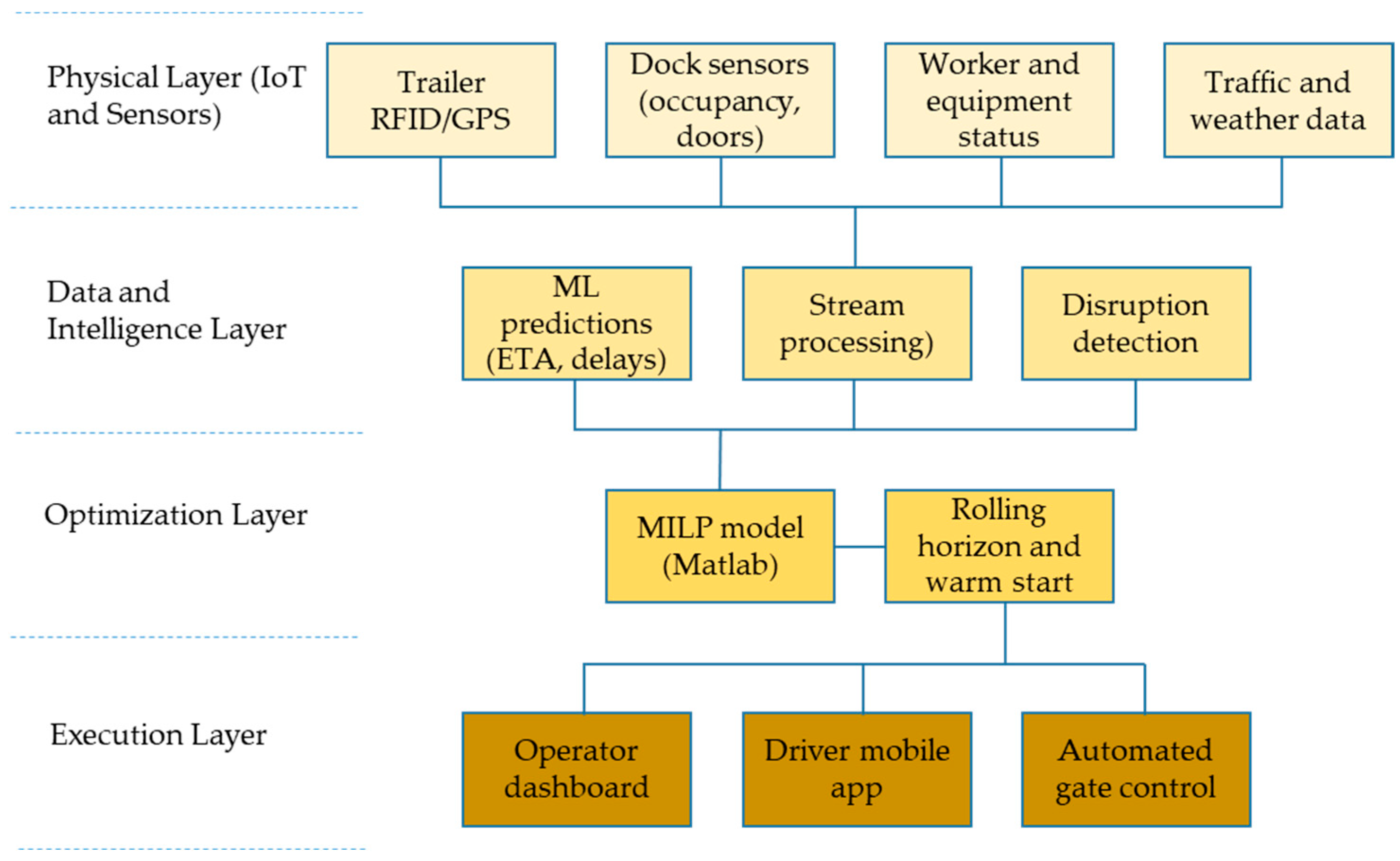
Figure 5 illustrates the conceptual framework of the proposed adaptive real-time planning system, which integrates Industry 4.0 technologies with mathematical optimization (MILP solved with Matlab R2025b). The system is designed as a cyber–physical decision-support loop, where digital data streams from the physical environment are continuously collected, processed, and transformed into actionable operational decisions.

At the first stage, IoT and sensor networks deployed throughout the cross-docking terminal monitor key operational parameters, such as trailer arrivals, dock occupancy, gate availability, handling progress, and unexpected disruptions (e.g., vehicle delays or equipment breakdowns). These data are transmitted in real time into a centralized data stream management system, ensuring that the decision-support layer always has the most recent information.

In the second stage, machine learning models are applied to generate predictive insights from the incoming data. For example, expected times of arrival (ETA) for inbound trailers can be estimated based on live traffic conditions, while the probability of delays or disruptions can be inferred from historical patterns. These predictive outputs provide a forward-looking dimension to the decision-making process, enabling the system not only to react to events as they occur but also to anticipate and prepare for potential disruptions.

The third stage is the mathematical optimization layer, where the updated and enriched data serve as input to a Mixed-Integer Linear Programming (MILP) model implemented in Matlab. The MILP formulation captures the trailer-to-dock assignment problem with constraints such as dock capacity, time windows, processing times, precedence relations between inbound and outbound flows, and resource availability. Depending on the operational priorities, the model can minimize trailer idle times, reduce delays, maximize dock utilization, or balance multiple performance criteria. Matlab solves the optimization problem under strict time limits, producing feasible and near-optimal solutions within seconds. Warm-start techniques and rolling-horizon optimization further ensure that the solver can be re-executed frequently as new data arrive, maintaining real-time responsiveness.

The output of the optimization step is a set of dynamic dock assignments, specifying in real time which trailer should be allocated to which dock and when. These assignments are communicated to the operational floor via terminal information systems such as large-screen displays, mobile applications for drivers, or automated gate-control systems. This creates a closed feedback loop. When new events occur in the physical system (e.g., a trailer arriving late), the sensors update the data stream, predictions are recalculated, the optimization is re-run, and revised dock assignments are generated almost instantly.

This tight integration between Industry 4.0 technologies (IoT, real-time data analytics, machine learning) and optimization methods (MILP solved in Matlab) provides a robust and adaptive decision-support system for high-throughput cross-docking terminals. By continuously sensing, predicting, and optimizing in real time, the system embodies the principles of Industry 4.0 and offers a pathway toward significantly enhanced operational efficiency, responsiveness, and resilience in next-generation logistics hubs.

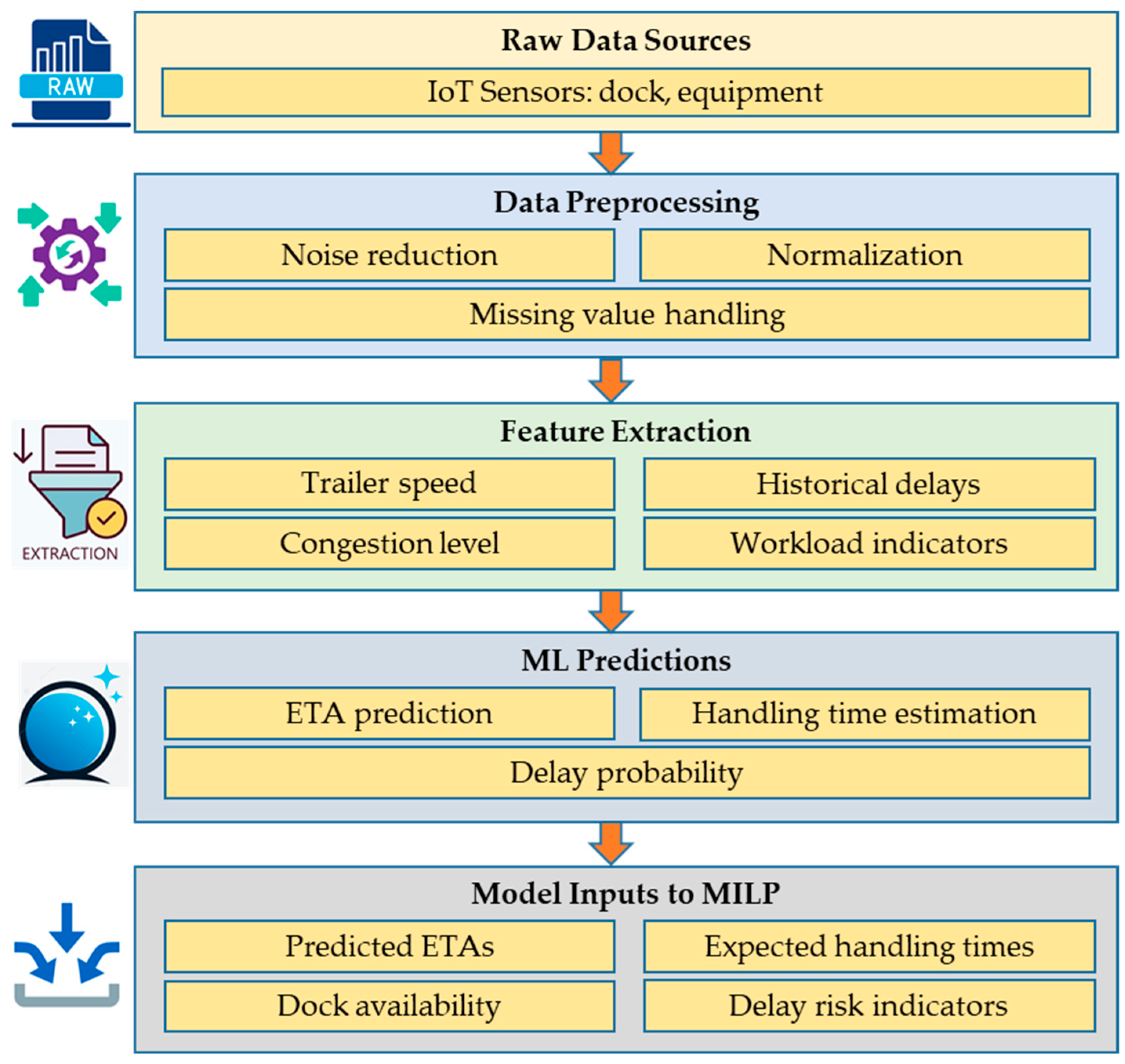
The Data & Intelligence Layer (Figure 6) plays a central role in transforming heterogeneous Industry 4.0 data streams into structured, actionable information that can be used by the optimization engine. It ensures that the optimization model is not only driven by raw sensor data but also enriched with predictive insights derived from advanced analytics and machine learning techniques. This layer can be divided into five sequential steps.

• Raw Data Sources: The process begins with the continuous acquisition of raw data from multiple origins. IoT sensors monitor dock occupancy, door status, and the availability of handling equipment in real time. GPS and RFID systems provide updates on trailer locations and expected arrivals. In addition, external feeds such as traffic congestion reports and weather forecasts supply contextual information that often affects arrival reliability and handling performance. While this diversity of sources ensures a holistic view of the terminal environment, it also introduces heterogeneity and noise.
• Data Preprocessing: Since raw operational data is often incomplete or inconsistent, preprocessing is essential. At this stage, erroneous signals are filtered out, missing values are estimated or imputed, and data are normalized to align different scales and units. Through these transformations, the system ensures that subsequent analytics operate on consistent and reliable inputs.
• Feature Extraction: Once cleaned, the data is enriched with engineered features that capture higher-level operational characteristics. From GPS trajectories, trailer speed profiles are derived, while traffic data is used to estimate congestion levels. Historical logs provide insights into recurring delay patterns, and operational records yield workload indicators such as trailer density per dock or operator utilization across shifts. These abstractions allow predictive models to detect complex patterns that cannot be inferred from raw data alone.
• Machine Learning Predictions: Using the extracted features, specialized machine learning models generate predictive insights that extend the time horizon of situational awareness. These models forecast estimated times of arrival for inbound trailers, quantify the probability of delays under varying conditions, and estimate handling times based on workload intensity and historical performance. The predictive layer thus converts static operational snapshots into forward-looking intelligence, enabling the system not only to react but also to anticipate.
• Model Inputs to MILP: Finally, the predictions are translated into structured parameters for the optimization model. Forecasted arrival times are represented as time-window constraints, expected handling times become service-duration parameters, dock availability is modeled as resource capacity, and delay risk indicators are incorporated either as penalty coefficients or robustness terms in the objective function. In this way, the MILP optimization layer receives inputs that are simultaneously current and predictive, equipping it to generate adaptive and resilient trailer-to-dock assignment plans.

3.2. Mathematical Model

This section presents a detailed mathematical model for the adaptive real-time assignment of trailers to docks in high-throughput cross-docking terminals. For each set of constraints and the objective function, we provide both the formal mathematical formulation and an explanatory interpretation.

Sets and indices used in the model are the followings:

• $I=\left\{1,\dots n_I\right\}$: set of inbound trailers (index i),
• $O=\left\{1,\dots n_O\right\}$: set of outbound trailers (index o),
• $D^{in}=\left\{1,\dots m_{in}\right\}$: set of inbound docks (index d),
• $D^{out}=\left\{1,\dots m_{out}\right\}$: set of outbound docks (index d),
• $T=\left\{1,\dots H\right\}$: discrete time slots (index t), each slot has a length $\Delta$, e.g., 5 min,
• Parameters used in the model are the followings:
• $a_i^I$: arrival time slot of inbound trailer i,
• $p_i^I$: processing duration of inbound trailer i (in slots),
• $a_o^O$: arrival time slot of outbound trailer o,
• $p_o^O$: processing duration of outbound trailer o (in slots),
• $u_{d,t}^{in}\in \left\{\mathrm{0,1}\right\}$: availability of inbound dock d at time t,
• $u_{d,t}^{out}\in \left\{\mathrm{0,1}\right\}$: availability of outbound dock d at time t,
• $Q_{i,o}\in \left\{\mathrm{0,1}\right\}$: precedence relation ($Q_{i,o}=1$ if outbound o requires inbound i to be completed first),
• ${due}_i^I$: deadline (latest desired completion) for inbound i,
• ${due}_o^O$: deadline for outbound o,
• $W_i^{max,I}$: maximum allowed waiting time for inbound i,
• $W_o^{max,O}$: maximum allowed waiting time for outbound o,
• $L_i^{max,I}$: maximum allowed tardiness for inbound i,
• $L_o^{max,O}$: maximum allowed tardiness for inbound o,
• $A_{d,i}^{in}\in \left\{\mathrm{0,1}\right\}$: compatibility ($A_{d,i}^{in}=1$ if inbound i can be processed at dock d),
• $A_{d,o}^{out}\in \left\{\mathrm{0,1}\right\}$: compatibility ($A_{d,o}^{out}=1$ if outbound o can be processed at dock d),
• $\alpha ,\beta$: weights for the objective function,
• $\Delta$: length of a time slot (in minutes).

The decision variables of the optimization problem are the followings:

• $x_{i,d,t}\in \left\{\mathrm{0,1}\right\}$: $x_{i,d,t}=1$ if inbound i starts processing at dock d in time slot t, otherwise $x_{i,d,t}=0$,
• $y_{o,d,t}\in \left\{\mathrm{0,1}\right\}$: $y_{o,d,t}=1$ if outbound o starts processing at dock d in time slot t, otherwise $y_{o,d,t}=0$,
• $S_i^I\ge 0$: start time of inbound i,
• $C_i^I\ge 0$: completion time of inbound i,
• $S_o^O\ge 0$: start time of outbound o,
• $C_o^O\ge 0$: completion time of outbound o,
• $L_i^I\ge 0$: tardiness of inbound i,
• $L_o^O\ge 0$: tardiness of outbound o.

The objective balances three operational goals: minimizing the waiting time of inbound trailers, minimizing tardiness of inbound trailers, and minimizing tardiness of outbound trailers. By tuning the weights α and β, operators can emphasize inbound efficiency or outbound service level.

$$\alpha ·\sum _{i\in I}\left(S_i^I-a_i^I\right)+\alpha ·\sum _{i\in I}{L}_i^I+\beta ·\sum _{o\in O}\left(S_o^O-a_o^O\right)+\beta ·\sum _{o\in O}{L}_o^O\to min.$$

(1)

where $\alpha$ is the weighting factor for inbound delays, $S_i^I$ is the starting time slot of inbound operation i, $a_i^I$ is the arrival time slot of inbound trailer i, $L_i^I$ is the tardiness of inbound i, $\beta$ is the weighting factor for outbound delays, $S_o^O$ is the starting time slot of outbound operation o, $a_o^O$ is the arrival time slot of outbound trailer o, $L_o^O$ is the tardiness of outbound o, $S_i^I=S_i^I\left(x_{i,d,t}\right)$ and $S_o^O=S_o^O\left(y_{o,d,t}\right)$.

The first summation penalizes inbound trailers that remain idle after their arrival, representing under-utilization of resources. The second term measures inbound tardiness, capturing late completion of inbound operations relative to deadlines. The third term measures outbound tardiness, directly affecting the service level for outbound deliveries. The objective is additive, so each trailer contributes independently, which makes the trade-offs transparent and tunable.

Constraint 1 defines the single start constraint. Each trailer can only start processing once, either at a single dock and a single time slot. This constraint prevents multiple assignments of the same trailer.

$$\forall i\in I: \sum _{d\in D^{in}}\sum _{t\in T}{x}_{i,d,t}\le 1,$$

(2)

$$\forall o\in O: \sum _{d\in D^{out}}\sum _{t\in T}{y}_{o,d,t}\le 1,$$

(3)

where decision variable $x_{i,d,t}$ indicated, whether inbound trailer i starts processing at dock d in time slot t, $d\in D^{in}$ is the set of inbound docks, decision variable $y_{o,d,t}$ indicated, whether inbound trailer o starts processing at dock d in time slot t, and $d\in D^{out}$ is the set of outbound docks.

These inequalities ensure that each inbound trailer is assigned to at most one inbound dock and each outbound trailer to at most one outbound dock.

Constraint 2 defines the start, completion, and arrival related conditions. The start and completion times of each trailer are defined as linear functions of the binary assignment variables. Trailers cannot begin processing before their arrival time.

$$\forall i\in I: S_i^I=\sum _{d\in D^{in}}\sum _{t\in T}t·x_{i,d,t},$$

(4)

$$\forall i\in I: C_i^I=S_i^I+p_i^I-1,$$

(5)

$$\forall i\in I: S_i^I\ge a_i^I$$

(6)

$$\forall o\in O: S_o^O=\sum _{d\in D^{out}}\sum _{t\in T}t·y_{o,d,t},$$

(7)

$$\forall o\in O: C_o^O=S_o^O+p_o^O-1,$$

(8)

$$\forall o\in O: S_o^O\ge a_o^O.$$

(9)

where $C_i^I$ is the completion time slot of inbound i, $p_i^I$ is the processing duration of inbound trailer i (in time slots), where $C_o^O$ is the completion time slot of outbound o, $p_o^O$ is the processing duration of outbound trailer o (in time slots).

These constraints tie the abstract decision variables to real operations. For example, if an inbound trailer starts at time t, its completion is determined by its processing duration. The ‘−1’ ensures correct inclusive counting of discrete slots.

Constraint 3 focuses on dock capacity. Each dock can serve at most one trailer at a time, and only if it is available. The coverage-based formulation accounts for ongoing processing across multiple slots.

$$\forall d\in D^{in},t\in T: \sum _{i\in I}\sum _{\tau =\mathrm{m}\mathrm{a}\mathrm{x}(1,t-p_i^I+1)}{x}_{i,d,\tau }\le u_{d,t}^{in},$$

(10)

$$\forall d\in D^{out},t\in T: \sum _{o\in O}\sum _{\tau =\mathrm{m}\mathrm{a}\mathrm{x}(1,t-p_o^O+1)}{y}_{o,d,\tau }\le u_{d,t}^{out},$$

(11)

where $u_{d,t}^{in}$ is the availability of inbound dock d at time t, and $u_{d,t}^{out}$ is the availability of outbound dock d at time t.

If a trailer starts earlier and overlaps with the current slot t, it is considered active. The dock availability parameter u enforces planned closures or pre-reservations, preventing usage during those slots.

Constraint 4 considers the precedence-relations. Some outbound trailers depend on the completion of specific inbound trailers. These precedence constraints capture synchronization of material flows across docks.

$$\forall \left(i,o\right)with Q_{i,o}=1: S_o^O\ge C_i^I,$$

(12)

where $Q_{i,o}$ is the precedence relation.

If trailer o requires trailer i, then o cannot start until i has finished. This ensures logical consistency between inbound unloading and outbound loading activities.

Constraint 5 focuses on tardiness. Tardiness variables measure the extent to which a trailer misses its deadline. They are defined relative to completion time and due date.

$$\forall i\in I: L_i^I\ge C_i^I-{due}_i^I \bigwedge L_i^I\ge 0,$$

(13)

$$\forall o\in O: L_o^O\ge C_o^O-{due}_o^O \bigwedge L_o^O\ge 0.$$

(14)

where ${due}_i^I$: is the deadline (latest desired completion) for inbound i, ${due}_o^O$ is the deadline for outbound o, $L_i^I$ is the tardiness of inbound i, and $L_o^O$ is the tardiness of outbound o.

If completion occurs before the due date, tardiness is zero. Otherwise, tardiness is the positive difference. This formulation linearizes the $max(0,lateness)$ function.

Constraint 6 takes the maximum waiting time into consideration. Waiting time is the difference between trailer arrival and actual start. This constraint enforces an upper bound to avoid excessive queuing in the yard.

$$\forall i\in I: S_i^I-a_i^I\le W_i^{max,I},$$

(15)

$$\forall o\in O: S_o^O-a_o^O\le W_o^{max,O}.$$

(16)

where $W_i^{max,I}$ is the maximum allowed waiting time slot for inbound i, and $W_o^{max,O}$ is the maximum allowed waiting time slot for outbound o.

By restricting waiting, the model reflects operational policies such as limited yard space or customer service commitments.

Constraint 7 focuses on maximum tardiness. Besides penalizing tardiness in the objective, hard upper bounds may be set to enforce service level guarantees.

$$\forall i\in I: L_i^I\le L_i^{max,I},$$

(17)

$$\forall o\in O: L_o^O\le L_o^{max,O}.$$

(18)

where $L_i^{max,I}$ is the maximum allowed tardiness for inbound i, and $L_o^{max,O}$ is the maximum allowed tardiness for inbound o.

This ensures that no trailer can exceed its maximum permissible delay, regardless of trade-offs in the objective.

Constraint 8 focuses on the compatibility of docks. Not every trailer can be served at every dock. Compatibility matrices restrict assignments to feasible dock-trailer pairs.

$$\forall d\in D^{in},i\in I: \sum _{t\in T}{x}_{i,d,t}\le A_{d,i}^{in},$$

(19)

$$\forall d\in D^{out},o\in O: \sum _{t\in T}{x}_{o,d,t}\le A_{d,o}^{out},$$

(20)

where $A_{d,i}^{in}$ is the compatibility of inbound trailer i and inbound dock d, $A_{d,o}^{out}$is the compatibility of outbound trailer o and outbound dock d.

If a trailer is not compatible with a dock, the binary parameter A forces all assignment variables for that pair to zero. This captures real-world constraints such as size limits, equipment requirements, or hazardous material handling.

In the proposed MILP formulation, the transportation phase is considered external to the scheduling process. Accordingly, the arrival time (ETA) of each trailer is used as an input parameter rather than being derived from distance or travel speed. This design choice allows the model to operate in real time: as soon as an updated ETA becomes available, reflecting traffic congestion, routing decisions, or time-of-day effects; the scheduling is re-optimized without modifying the underlying formulation.

4. Results

This section begins with the presentation of the parameters of the investigated model. Thereafter, a detailed description is provided on the outcomes of conventional optimization as well as those obtained through adaptive, real-time optimization.

4.1. Parameters of the Investigated Model

During the optimization, a case study with the following input data was examined:

• the length of a time slot: $\Delta =5 \mathrm{m}\mathrm{i}\mathrm{n}$,
• the number of inbound trailers within the time-window of the analysis: $n_I=12,$
• the number of outbound trailers within the time-window of the analysis: $n_O=8,$
• the number of inbound docks $m_{in}=6,$
• the number of outbound docks $m_{out}=4,$
• the weights for the objective function $\alpha =1, \beta =1,$
• the precedence matrix:

$$Q=\left[\begin{array}{cccccccc}1& 0& 0& 1& 0& 1& 0& 0\\ 1& 1& 0& 0& 1& 0& 1& 0\\ 0& 1& 0& 0& 1& 0& 0& 1\\ 0& 0& 1& 0& 0& 1& 1& 0\\ 0& 0& 1& 1& 0& 0& 1& 0\\ 0& 0& 0& 1& 0& 1& 0& 0\\ 0& 0& 0& 0& 1& 0& 0& 0\\ 1& 0& 0& 0& 1& 1& 0& 0\\ 0& 1& 0& 1& 0& 0& 1& 0\\ 0& 0& 1& 1& 0& 1& 0& 0\\ 0& 0& 0& 0& 1& 0& 1& 0\\ 0& 0& 0& 0& 0& 0& 0& 1\end{array}\right],$$

(21)

• the arrival time, processing time and due time of inbound trailers (see

  Table 6. Input parameters of inbound trailers.

  Parameters		ID of Inbound Trailers
  Name	Symbol	1	2	3	4	5	6	7	8	9	10	11	12
  Arrival time	$a_i^I$	9	10	14	18	20	12	14	16	18	20	15	20
  Processing time	$p_i^I$	7	6	4	7	5	6	8	5	7	6	5	6
  Due time	${due}_i^I$	19	19	21	28	28	21	25	24	28	29	23	29

  ),
• the arrival time, processing time and due time of outbound trailers (see

  Table 7. Input parameters of outbound trailers.

  Parameters		ID of Outbound Trailers
  Name	Symbol	1	2	3	4	5	6	7	8
  Arrival time	$a_o^O$	11	11	12	9	11	13	18	15
  Processing time	$p_o^O$	6	7	5	6	8	7	6	7
  Due time	${due}_o^O$	34	35	34	32	36	37	41	39

  ),
• prebooking parameters of inbound and outbound docks (see

  Table 8. Prebooking parameters of inbound and outbound docks.

  Prebooking Time	Inbound Docks							Outbound Docks
  	1	2	3	4	5	6	6	1	2	3	3
  from time slot	8	1	10	1	14	10	16	20	10	10	35
  to time slot	11	12	22	6	22	12	20	25	15	20	40

  ).

All experiments were run on a workstation equipped with an Intel i9 CPU and 128 GB RAM under Windows 11. Each optimization run finished within about 13 s.

The operating system was Microsoft Windows 11 Enterprise 64-bit (Build 26100), configured with Hungarian regional settings. The workstation employed DirectX 12 as the graphics subsystem. The system supported Miracast wireless display features, while hybrid graphics functionality (Microsoft Graphics Hybrid) was not enabled.

4.2. Conventional Solution

In the conventional approach, inbound trailers are assigned to inbound docks in the order of their arrival (FCFS = first-come first-served).

Figure 7 shows the schedule of inbound and outbound trailers. In the original schedule, inbound trailers are mostly served in the earlier timeslots, while outbound trailers are pushed towards the later part of the horizon. There is little overlap between the two groups, so the flow shifts quite distinctly from inbound to outbound handling. The overall makespan is relatively long, with the last outbound trailer (Out8) only finishing around timeslot 45. Small idle gaps can also be observed between certain trailers, which indicates that dock capacity is not used at its maximum efficiency throughout the entire period (see Figure 7).

Figure 8 shows the schedule of inbound and outbound docks. In the first schedule, the inbound trailers are spread across the six input docks, but the allocation is somewhat uneven, which is caused by the prebooking. For example, InDock 4 is heavily loaded, handling multiple trailers (In1, In3, In8, In12), while some other docks are less utilized. The sequence of inbound handling extends up to around timeslot 30. On the outbound side, several docks are active, but OutDock 2 and OutDock 1 carry most of the load, and the overall completion time stretches close to timeslot 45. While the plan respects pre-bookings, there are noticeable imbalances in dock usage (see Figure 8).

Figure 9 shows the delays of trailers. In the first scenario, several trailers experience noticeable delays. Among inbound trailers, In9 and In12 are each delayed by 1 timeslot. On the outbound side, delays are more significant: Out4 is delayed by 2, Out5 by 1, Out6 by 4, and Out8 by as much as 5 timeslots. This distribution shows that outbound trailers suffer the most from delays, with multiple cases of extended waiting time. Overall, the system performance is weakened by a relatively high total delay, especially concentrated at the end of the schedule (see Figure 9).

Figure 10 shows the utilization of the inbound docks. The average utilization of the inbound docks (excluding pre-bookings) is 68%. Within the observed time window, one dock was occupied 6.7% of the time, two docks 23.3%, three docks 10%, four docks 3.3%, five docks 23.3%, and all six docks were occupied 33.3% of the time. The average number of occupied docks was 4.13, with a standard deviation of 2.1.

Figure 11 shows the utilization of outbound docks. The average utilization of the out-bound docks (excluding pre-bookings) is 57%. Within the observed time window, one out-bound dock was occupied 37.1% of the time, two docks 25.7%, three docks 5.7%, and all four outbound docks were occupied 31.4% of the time. The average number of occupied outbound docks was 2.31, while the standard deviation of this value was 1.27.

4.3. Adaptive, Real-Time Optimization

In the case of the adaptive, real-time optimization, the optimization problem was formulated as a mixed-integer linear program (MILP) and solved using MATLAB’s intlinprog solver, which employs the HiGHS optimization engine. The solution process follows a branch-and-bound (B&B) framework, enhanced with presolve techniques, cutting planes, and symmetry detection to improve computational efficiency.

At the outset, the solver applied a presolve phase, during which redundant constraints were eliminated, inactive variables were detected, and implied integer variables were reformulated. This step significantly reduced the dimensionality of the problem by lowering the number of constraints, variables, and nonzero coefficients in the constraint matrix. Multiple restarts of the presolve routine were carried out, reflecting the solver’s dynamic approach to further simplifying the model as new information became available during the search.

The main solution phase was conducted using branch-and-bound, in which the feasible region is recursively partitioned into smaller subproblems (nodes). At each node, a relaxation of the MILP is solved as a linear program (LP), providing a lower (dual) bound on the objective function. The solver then compares this bound with the best feasible (primal) solution identified so far, gradually closing the optimality gap. The process is supported by cutting plane generation, strong branching strategies, and heuristic search methods that accelerate the discovery of good feasible solutions. Symmetry detection was also applied, identifying orbitopes that reduce the number of equivalent solutions explored, further improving efficiency.

Throughout the run, the solver reported the evolution of the best primal solution, the dual bound, and the relative gap. The iterative refinements of the model (seen in successive restarts with progressively fewer binary variables) demonstrate how the solver adaptively tightened the formulation. The optimization terminated once the relative optimality gap fell below the tolerance threshold (0.01%), at which point the optimal solution was proven. The total runtime was approximately 12.8 s, including 2.6 s spent in presolve.

In summary, the solver combined presolve reductions, advanced branch-and-bound techniques, cutting planes, and symmetry handling to efficiently navigate the large-scale MILP and ultimately guarantee global optimality of the integer solution.

In the context of our study, real time does not mean instantaneous or continuous sub-second optimization, but rather the ability of the system to adaptively re-optimize decisions in response to live operational data within the short time frame required by terminal operations.

As described in Section 3.1 and Section 4.3 of the paper, the proposed framework operates in a rolling-horizon, event-driven mode. Incoming data from IoT sensors, GPS, and terminal information systems are continuously monitored. Whenever a relevant change occurs (e.g., trailer delay, dock unavailability, or congestion), the system updates the model parameters and re-runs the MILP optimization. The computational time (approximately 12–13 s per run) is well within the operational decision cycle of a high-throughput terminal, where trailer events typically occur on a minute-level timescale.

Therefore, in our terminology, real time refers to the operational responsiveness of the decision-support loop rather than to a solver that produces an immediate solution without computation time.

While MATLAB’s intlinprog solver indeed uses a branch-and-bound framework, it is sufficiently fast for mid-size MILP instances (as shown in our numerical experiments) and can be executed repeatedly in near real time. In practice, this solver forms the optimization core of a cyber–physical control loop that integrates live data acquisition, predictive analytics, and frequent re-optimization. Thus, the contribution lies not in developing a new solver, but in designing an adaptive planning architecture that maintains up-to-date trailer assignments through repeated, fast MILP re-optimizations based on live inputs.

Figure 12 shows the schedule of inbound and outbound trailers, while Figure 13 shows the schedule of inbound and outbound docks. In the optimized schedule, inbound and outbound trailers are interleaved more effectively. Starting from around timeslot 20, both types of trailers are being processed in parallel, which creates a smoother transition and balances the workload. The allocation of trailers is tighter, leaving fewer idle periods, and the overall makespan is reduced: the last outbound trailer finishes around timeslot 40 instead of 45. This leads to a more efficient use of resources, higher throughput, and a more balanced schedule compared to the original version (see Figure 12).

In the optimized schedule, the distribution of trailers across docks is more balanced. For inbound, heavy clustering at InDock 4 is reduced, with trailers being spread more evenly across InDock 2, InDock 3, and InDock 5. This creates a smoother flow, with inbound operations finishing earlier and closer together in time. On the outbound side, the workload is also more evenly split between the four docks, reducing pressure on OutDock 1 and 2 compared to the first version. As a result, the final outbound trailer finishes earlier, around timeslot 40, which shortens the overall makespan. The optimized plan therefore achieves a more efficient use of dock capacity and reduces idle times, while still honoring the pre-bookings (see Figure 13).

Figure 14 shows the delays of trailers. In the optimized scenario, the number and size of delays are reduced. Only one inbound trailer (In7) is affected, with a delay of 3 timeslots. For outbound trailers, Out4 has a small delay of 1 and Out6 has a delay of 3. Compared to the first version, there are fewer trailers experiencing delays, and no extreme cases like the 5-slot delay seen earlier. The result is a more balanced and predictable schedule, with significantly lower overall delay impact (see Figure 14).

Figure 15 shows the utilization of the inbound docks in the case of adaptive real-time assignment. The average utilization of the inbound dock (excluding pre-bookings) is 71%. Within the observed time window, one dock was occupied 6.9% of the time, two docks 24.1%, three docks 6.9%, four docks 3.4%, five docks 17.2%, and all six docks were occupied 41.4% of the time. The average number of occupied docks was 4.24, while the standard deviation of this value was 1.88. Comparing the adaptive solution and the conventional baseline algorithm (FCFS), the average dock utilization increased from 68% to 71%, and periods of full occupancy rose from 33.3% to 41.4%. The standard deviation decreased from 2.1 to 1.88, indicating a more balanced and stable workload. Overall, the adaptive optimization achieved higher utilization and smoother performance than the conventional FCFS scheduling.

Figure 16 shows the utilization of outbound docks in the case of adaptive real-time assignment. The average utilization of the outbound dock is 62%. Within the observed time window, one outbound dock was occupied 28.1% of the time, two docks 34.4%, three docks 0%, and all four outbound docks were occupied 37.5% of the time. The average number of occupied outbound docks was 2.47, while the standard deviation of this value was 1.27. For outbound operations, average dock utilization increased from 57% to 62%, while periods of full occupancy rose from 31.4% to 37.5%. The average number of occupied docks grew from 2.31 to 2.47, showing a more even workload distribution. Overall, the adaptive approach resulted in higher utilization, reduced idle times, and greater operational balance compared to the conventional FCFS method.

The above-mentioned numerical results show that applying an adaptive, real-time assignment of inbound and outbound trailers to the corresponding docks can significantly improve the utilization of the cross-docking terminal.

5. Discussion

The numerical results provide clear evidence of the advantages of adaptive, real-time assignment in cross-docking operations. Compared to the conventional first-come-first-served approach, the proposed optimization framework achieves both higher utilization of docks and a significant reduction in trailer delays.

On the inbound side, the average dock utilization increased from 68% to 71%, while the share of time when all six inbound docks were simultaneously occupied rose from 33.3% to 41.4%. At the same time, the distribution of dock use became more balanced: the average number of simultaneously occupied inbound docks increased slightly from 4.13 to 4.24, while the standard deviation decreased from 2.1 to 1.88. These indicate that the adaptive strategy leads to a steadier workload distribution and better exploitation of terminal capacity.

Outbound operations show similar improvements. Under conventional scheduling, the average utilization of outbound docks was 57%, with an average of 2.31 docks occupied and a standard deviation of 1.27. With adaptive assignment, utilization increased to 62%, the average number of occupied docks rose to 2.47, and periods with full use of all four docks expanded from 31.4% to 37.5%. These changes demonstrate that outbound flows, which are often more prone to delays due to dependencies on inbound unloading, can be stabilized by continuous re-optimization.

Trailer delays also decreased notably. In the conventional plan, multiple outbound trailers suffered significant delays, with some waiting up to five time slots beyond their due time. In contrast, the adaptive solution reduced delays to only a few cases (e.g., one inbound trailer with a three-slot delay and two outbound trailers with minor delays). The overall schedule shortened as well, with the makespan reduced from approximately 45 time slots to 40 time slots, reflecting a faster and more efficient flow through the terminal.

Although the overall improvement compared to the FCFS baseline appears moderate (around 3% at the inbound dock and 5% at the outbound dock), these results are obtained under real-time, event-driven operational conditions with strict resource constraints and uncertain trailer arrivals. In such environments, even a few percentage points of gain in dock utilization or makespan reduction can yield substantial operational and cost benefits when scaled to daily or annual throughput. More importantly, the proposed real-time optimization framework provides greater system stability and adaptability than FCFS, as it continuously re-optimizes upon each trailer arrival without requiring complete rescheduling. This capability ensures smoother coordination between inbound and outbound flows and reduces waiting-time variability; factors that are often more critical in practice than achieving larger improvements in static or offline optimization settings.

Therefore, the reported performance enhancement should be interpreted not only in terms of absolute numerical efficiency but also as evidence of robust, real-time decision support that improves responsiveness and operational resilience in dynamic terminal environments.

In practice, the adaptive method made the docks busier, reduced waiting times, and made the system less sensitive to delays. These improvements were consistent across both inbound and outbound flows.

From a managerial perspective, these results suggest that the adoption of real-time optimization tools can yield tangible benefits in terms of throughput, responsiveness, and predictability. Importantly, the system does not rely on static schedules but instead leverages live data to continuously re-allocate trailers, which is particularly advantageous in volatile logistics environments.

At the same time, some limitations should be acknowledged. The framework presupposes the availability of accurate real-time data streams from IoT, sensors, and information systems. In practice, data latency, missing values, or inconsistent updates may reduce the quality of the optimization input. Moreover, while the computational requirements of the MILP formulation were manageable in the tested scenario (solution times of approximately 12–13 s), scaling up to larger hubs with higher volumes may necessitate more advanced solver strategies, heuristic enhancements, or parallel computing resources.

Although vehicle routing (VRP) factors can influence transportation times, the current study focuses on dock scheduling and resource allocation after trailers’ arrival. The VRP impact is therefore implicitly reflected through real-time ETA updates, which incorporate the effects of route selection, congestion, and time of day. Whenever these ETAs change, the model re-optimizes the dock assignment instantly. This approach keeps the MILP formulation tractable while maintaining realistic responsiveness to dynamic transportation conditions.

In conclusion, the discussion of the numerical results confirms that adaptive, real-time assignment is a promising direction for improving the performance of high-throughput cross-docking terminals. Integrating live data with optimization turned out to be practical for daily terminal operations. It showed that mathematical models can be useful in real-time settings if updated continuously.