Abstract
In this work, explicit Two-Derivative Runge–Kutta methods of the general case (that use several evaluations of the right-hand side function and its derivative per step) are considered. In order to address problems of orbital or oscillatory character, we develop methods with frequency-dependent coefficients. We construct three exponentially/trigonometrically fitted methods following two approaches suggested by Vanden Berghe and Simos. Also, we construct a phase-fitted and amplification-fitted method. The efficiency of the new modified methods is demonstrated by numerical examples.
Keywords:
Two Derivative Runge–Kutta methods; trigonometrical fitting; dispersion error; dissipation error MSC:
65L05; 65L06
1. Introduction
In this work, we consider the initial value problem
For the numerical integration of this system of an ordinary differential equation, apart from classical methods, the construction of special methods that take into consideration properties of the solution of specific problems has been proposed by many researchers and are still of great interest. A frequent characteristic of many physical phenomena is the oscillatory or exponential behavior. This is the case in many areas of applied science, such as chemistry, molecular dynamics, celestial mechanics. When working with oscillatory problems, special attention should be given to the frequency as well as the phase of the oscillation. The first multistep method to be considered for the integration of the problems with oscillatory behavior of the solution was proposed by Gautschi, who developed special linear multistep methods [1] based on trigonometric polynomials. Lyche [2] gave the theoretical framework for exponential/trigonometrical (EF/TF) fitting multistep methods, which was followed by the work of Raptis and Allison [3], who derived EF/TF methods for the numerical solution of the Schrödinger equation. Since then, a lot of work has been devoted to the EF/TF multistep methods, especially for second-order ODEs. These methods have variable coefficients dependent on the frequency; therefore, a good estimate of the frequency is needed. EF/TF Runge–Kutta (RK) methods first appeared quite later in 1998 by Paternoster [4], Simos [5] and Vanden Berghe et al. [6]. The idea of phase-lag appears for the first time in the literature in the work of Brusa and Nigro [7]. Van der Houwen and Sommeijer [8] provided a definition for the phase-lag and dissipation for RK methods based on the stability function and constructed RK methods to address problems with oscillating solution. An estimate of the frequency is not needed since these methods have constant coefficients. Simos [9] derived an RK method with a phase-lag of order infinity (phase-fitted) with frequency-dependent coefficients.
Runge–Kutta methods have been used for the numerical integration of problem (1) since the beginning of the previous century. Also, RK-type methods have been developed as Runge–Kutta-Nyström (RKN), Partition Runge–Kutta (PRK), and two-step hybrid Runge–Kutta methods (TSRK). An important category of RK-type methods are the Two-Derivative Runge–Kutta methods (TDRK), which were introduced by Chan and Tsai in [10], where also an order of conditions that were derived in the framework of Butcher’s theory [11]. These methods also include the computation of the second derivative at intermediate points. The order of a TDRK method can be achieved using significantly fewer stages compared to RK methods. Also, a special class of explicit TDRK (SETDRK) methods was considered when the computation of f values at intermediate points was not used. Apart from TDRK methods, researchers also presented Two-Derivative Runge–Kutta-Nyström methods [12] and Two-Derivative Two-Step Runge–Kutta Methods [13].
A lot of research has been devoted to the construction of SETDRK methods for oscillatory problems in a similar manner to RK methods. At first, trigonometrically fitted SETDRK methods were considered by Zhang et al. [14], and Fang et al. [15], Fang and You [16], who constructed phase-fitted SETDRK methods. Also, phase-fitted and amplification-fitted SETDRK methods were constructed by Ahmad et al. [17]. Additionally, methods with reduced phase error and amplification error were considered by Fang et al. [18].
For the first time general explicit TDRK methods, that use several f evaluations at each step, for oscillatory problems were considered by Monovasilis et al. in [19] and trigonometrically fitting conditions were derived. Kalogiratou et al. in [20] constructed methods with constant coefficients of the general case and algebraic order five as well as modified trigonometrically fitted methods. Conditions for algebraic order six were given by the authors in [21].
In this work, we focus on modified explicit TDRK methods of algebraic order six with special properties. We construct a phase fitted and amplification-fitted method, trigonometrically fitted methods based on two approaches: each stage approach and Simos’ approach [5,6]. The necessary background theory is given in Section 2 and Section 3; in Section 2 we give a brief presentation of TDRK methods, while in Section 3 we revise the theory of exponentially fitted TDRK methods. New methods are constructed in Section 4 and numerical results that illustrate the performance of the new methods are presented in Section 5.
2. Explicit Two Derivative Runge–Kutta Methods
TDRK methods defined in [10] are RK-type methods that also include the computation of the second derivative
at intermediate points.
An s stage TDRK method is in the form of
where the associated Butcher tableau is
where A and are matrices, and b and , c are vectors.
Let T be the set of rooted trees, then the real-valued functions are the order, symmetry, density, and elementary weight, respectively. Also, let be the vector of elementary weight functions. As in the case of Runge–Kutta methods the order conditions are derived by comparison of the Taylor series of the exact and the numerical solution, this implies that a method is of algebraic order p if for all rooted trees t with .
The vector of elementary weight functions is defined for the empty tree and for the tree of first order as , and for the trees of order by the recursion formula
where is the tree of order that results from by subtracting the root and is the tree of order that results from by subtracting the second-order tree .
The elementary weight for the tree of first order is defined as and for trees of order as
The stability function is
For periodic initial value problems it is important to consider the stability on the imaginary axis. The test problem with is used. As in the case of explicit RK methods the stability function can be written as
where and , are polynomials in of degree s. Generalizing the ideas of Van der Houwen and Sommeijer [8] for RK methods, the definition of the dispersion (or phase error) and the dissipation (or amplification error) for (2) are
where . For explicit methods
Vanden Berghe et al. in [6] introduced EF/TF RK methods that integrate exactly exponential functions at each internal stage. Following this idea, the authors in [19] considered explicit TDRK methods and gave the following conditions:
for each stage and for the final stage
where , z is the frequency of the problem.
3. New Methods
In this section, for the first time, we present the necessary theoretical results for constructing modified TDRK methods. In [5], Simos proposed modified RK methods for problems with oscillating or periodic solution, generalizing the ideas introduced by Lyche [2] for multistep methods.
Following the ideas in [5], method (2) is associated with the operator
where z is a continuously differentiable function.
The following definition is given in [5]
Definition 1.
A method is called exponential of order q if the associated linear operator L vanishes for any linear combination of the linearly independent functions where are real or complex numbers.
Remark 1.
If for then the operator L vanishes for any linear combination of .
We give the following theorem.
Theorem 1.
Proof.
Let
and , the elementary weight vector of elementary weight functions associated with these trees
Then,
For let then , , we want the linear operator L to vanish and obtain the following conditions
Since for , , we ask for the operator L to vanish for . Working similarly we obtain
for .
This generalizes the result given by the authors in [20]. □
For with real, the following trigonometrically fitting conditions are derived: ().
for r even
for r odd
The operator L vanishes for if the conditions are satisfied
The operator L vanishes for and if the conditions are also satisfied
4. Construction of the New Methods
Based on the methodology developed in [21], we constructed a sixth order method that will be used as the reference method.
From Equation (3), we modify the coefficients and for . In order to satisfy Equation (4), we modify two of the coefficients or for . We modify the above method using the each stage approach and found the following coefficients:
We refer to this method as NewTF1.
Applying Simos’ approach, we derive two modified methods. For the first modified method the linear operator L disappears for , i.e., satisfies (5). We refer to this method as NewTF2. For the second method, the linear operator L disappears for and , i.e., satisfies (5) and (6). We refer to this method as NewTF3.
The elementary weights can be found in terms of the elementary weight functions which for a method with stages are as follows:
For the new methods:
- NewTF2: we modify the coefficients from conditions (5), , ,
For NewTF2, the modified coefficients are as follows:
For NewTF3, the modified coefficients are as follows:
The next method is constructed so that the phase-lag error and the amplification error are nullified. We refer to this method as NewPF.
5. Numerical Results
In order to demonstrate the efficiency of the new modified methods NewTF1, NewTF2, NewTF3, NewPF we have tested them as well as the method with constant coefficients presented in the begining of the previous section (New) and the method constructed in [21] (Meth2). The last method (Meth2) was constructed by nullifying two extra terms of the phase-lag error and one term of the amplification error and .
The problems used are the inhomogeneous equation studied by van der Houwen and Sommeijer [8], the oscillatory linear system studied by Franco in [22], the almost periodic orbit problem studied by Stiefel and Bettis in [23] and the two body problem.
5.1. Problem 1
The inhomogeneous equation in [8]
where . The exact solution is . We choose and integration interval . In Figure 1, we see the efficiency of the methods (the maximum error of the solution) vs. CPU time for the inhomogeneous equation. Methods NewTF2 and NewTF3 constructed via the Simos’ approach are the most efficient followed by NewTF1 constructed via the each stage approach and the phase-fitted and amplification-fitted method NewPF. All variable coefficients methods have superior performance compared to the constant coefficients methods.
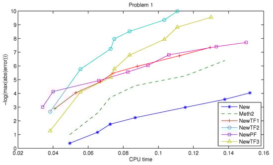
Figure 1.
Problem 1: Efficiency curves.
5.2. Problem 2
We consider the oscillatory linear system in [22]
The exact solution is
In Figure 2, the maximum error of the solution is presented in the interval .
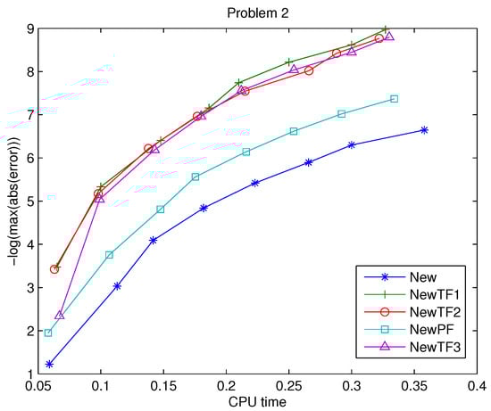
Figure 2.
Problem 2: Efficiency curves.
As we have seen in Problem 1, all modified methods have superior performance compared to the constant coefficients methods. The trigonometrically fitted methods have similar performance followed by NewPF.
5.3. Problem 3
We consider the Stiefel and Bettis problem:
The exact solution is
In Figure 3, the maximum error of the solution is presented .
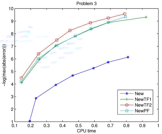
Figure 3.
Problem 3: Efficiency curves.
Here, again all modified methods have superior performance.
5.4. Problem 4
We consider the two body problem:
The exact solution is
For this problem method, NewTF1, constructed via the Vanden Berghe approach, shows excellent performance and gives an error order of for any step up to . All other methods have similar performance the error is for step .
6. Discussion and Conclusions
In this work, explicit two-derivative Runge–Kutta methods of the general case (that use several evaluations of the right-hand side function and its derivative per step) have been considered. We focus on methods with variable frequency-dependent coefficients for the numerical integration of problems with periodic or oscillatory behavior of the solution. An explict, sixth-order condition with five stages has been developed and based on this method, we derived three trigonometrically fitted methods using the fitting approach of Vanden Berghe and the fitting approach of Simos, also a phase-fitted and amplification method. For the first time, conditions for second exponential order for the general case are given in terms of the elementary weights. Numerical tests have been carried out on four test problems: the inhomogeneous equation studied by van der Houwen and Sommeijer [8], the oscillatory linear system studied by Franco in [22], the almost periodic orbit problem studied by Stiefel and Bettis in [23] and the two body problem. All modified methods show superior performance.
Author Contributions
All stages of the preparation of the manuscript have been carried out by both authors (T.M. and Z.K.). All authors have read and agreed to the published version of the manuscript.
Funding
This research received no external funding.
Data Availability Statement
Data are contained within the article.
Conflicts of Interest
The authors declare no conflicts of interest.
References
- Gautschi, W. Numerical Integration of Ordinary Differential Equations Based on Trigonometric Polynomials. Numer. Math. 1961, 3, 381–397. [Google Scholar] [CrossRef]
- Lyche, T. Chebyshevian multistep methods for ordinary differential equations. Numer. Math. 1972, 19, 65–75. [Google Scholar] [CrossRef]
- Raptis, A.D.; Allison, A.C. Exponential-Fitting Methods for the Numerical Solution of the Schrödinger Equation. Comput. Phys. Commun. 1978, 44, 95–103. [Google Scholar] [CrossRef]
- Paternoster, B. Runge-Kutta(-Nyström) Methods for ODEs with Periodic Solutions Based on Trigonometric Polynomials. Appl. Num. Math. 1998, 28, 401–412. [Google Scholar] [CrossRef]
- Simos, T.E. An exponentially-fitted Runge-Kutta method for the Numerical Integration of Initial-Value Problems with Periodic or Oscillating Solutions. Comput. Phys. Commun. 1998, 115, 1–8. [Google Scholar] [CrossRef]
- Vanden Berghe, G.; De Meyer, H.; Van Daele, M.; Van Hecke, T. Exponentially-fitted Explicit Runge-Kutta Methods. Comput. Phys. Commun. 1999, 123, 7–15. [Google Scholar] [CrossRef]
- Brusa, L.; Nigro, L. A One-Step Method for Direct Integration of Structural Dynamic Equations. Int. J. Numer. Methods Eng. 1980, 15, 685–699. [Google Scholar] [CrossRef]
- van der Houwen, P.J.; Sommeijer, B.P. Explicit Runge–Kutta (–Nyströom) methods with reduced phase errors for computing oscillating solutions. SIAM J. Numer. Anal. 1987, 24, 595–617. [Google Scholar] [CrossRef]
- Simos, T.E. A Runge-Kutta Fehlberg Method with Phase-Lag of Order Infinity for Initial-Value Problems with Oscillating Solution. Comput. Math. Appl. 1993, 25, 95–101. [Google Scholar] [CrossRef]
- Chan, R.P.K.; Tsai, A.Y.J. On Explicit Two-Derivative Runge-Kutta Methods. Numer. Algor. 2010, 53, 171–194. [Google Scholar] [CrossRef]
- Butcher, J.C. The Numerical Analysis of Ordinary Differential Equations; John Wiley Sons: Chichester, UK, 1987. [Google Scholar]
- Chen, Z.; Shi, L.; Liu, S.; You, X. Trigonometrically Fitted Two-Derivative Runge-Kutta-Nyström methods for second-order oscillatory differential equations. Appl. Numer. Math. 2019, 142, 171–189. [Google Scholar] [CrossRef]
- Okten Turaci, M.; Öziş, T. On Explicit Two-Derivative Two-Step Runge-Kutta Methods. Comp. Appl. Math. 2018, 37, 6920–6954. [Google Scholar] [CrossRef]
- Zhang, Y.; Che, H.; Fang, Y.; You, X. A New Trigonometrically Fitted Two-Derivative Runge-Kutta Method for the Numerical Solution of the Schrödinger Equation and Related Problems. J. Appl. Math. 2013, 2013, 937858. [Google Scholar] [CrossRef]
- Fang, Y.; You, X.; Ming, Q. Trigonometrically Fitted Two-Derivative Runge-Kutta Methods for Solving Oscillatory Differential Equations. Numer. Algor. 2014, 65, 651–667. [Google Scholar] [CrossRef]
- Fang, Y.; You, X. New Optimized Two-Derivative Runge-Kutta Type Methods for Solving the Radial Schrödinger Equation. J. Math. Chem. 2014, 52, 240–254. [Google Scholar] [CrossRef]
- Ahmad, N.A.; Senu, N.; Ismail, F. Phase-Fitted and Amplification-Fitted Higher Order Two-Derivative Runge-Kutta Method for the Numerical Solution of Orbital and Related Periodical IVPs. Math. Prob. Eng. 2017, 2017, 1871278. [Google Scholar] [CrossRef]
- Fang, Y.; Zhang, Y.; Wang, P. Two-derivative Runge-Kutta Methods with Increased Phase-lag and Dissipation Order for the Schrödinger Equation. J. Math. Chem. 2018, 56, 1924–1934. [Google Scholar] [CrossRef]
- Monovasilis, T.; Kalogiratou, Z.; Simos, T.E. Trigonometrical Fitting Conditions for Two Derivative Runge-Kutta Methods. Numer. Algor. 2018, 79, 787–800. [Google Scholar] [CrossRef]
- Kalogiratou, Z.; Monovasilis, T.; Simos, T.E. New Fifth-Order Two-Derivative Runge-Kutta Methods with Constant and Frequency-Dependent Coefficients. Math. Meth. Appl. Sci. 2019, 42, 1955–1966. [Google Scholar] [CrossRef]
- Kalogiratou, Z.; Monovasilis, T. Construction of Two-Derivative Runge-Kutta Methods of Order Six. Algorithms 2023, 16, 558. [Google Scholar] [CrossRef]
- Franco, J.M. A class of explicit two-step hybrid methods for second-order IVPs. J. Comput. Appl. Math. 2006, 187, 41–57. [Google Scholar] [CrossRef]
- Stiefel, E.; Bettis, D.G. Stabilization of Cowell’s method. Numer. Math. 1969, 13, 154–175. [Google Scholar] [CrossRef]
Disclaimer/Publisher’s Note: The statements, opinions and data contained in all publications are solely those of the individual author(s) and contributor(s) and not of MDPI and/or the editor(s). MDPI and/or the editor(s) disclaim responsibility for any injury to people or property resulting from any ideas, methods, instructions or products referred to in the content. |
© 2025 by the authors. Licensee MDPI, Basel, Switzerland. This article is an open access article distributed under the terms and conditions of the Creative Commons Attribution (CC BY) license (https://creativecommons.org/licenses/by/4.0/).