Bootstrap-Based Stabilization of Sparse Solutions in Tensor Models: Theory, Assessment, and Application

Abstract

This paper introduces BCenetTucker, a novel bootstrap-enhanced extension of the CenetTucker model designed to address the instability of sparse support recovery in high-dimensional tensor settings. By integrating mode-specific resampling directly into the penalized tensor decomposition process, BCenetTucker improves the reliability and reproducibility of latent structure estimation without compromising the model′s interpretability. The proposed method is systematically benchmarked against classical CenetTucker, Stability Selection, and Bolasso, using real-world gene expression data from the GSE13159 leukemia dataset. Across multiple stability metrics—including support-size deviation, average Jaccard index, inclusion frequency, proportion of stable support, and Stable Selection Index (SSI)—BCenetTucker consistently demonstrates superior robustness and structural coherence relative to competing approaches. In the real data application, BCenetTucker preserved all essential signals originally identified by CenetTucker while uncovering additional marginal yet reproducible features. The method achieved high reproducibility (Jaccard index = 0.975; support-size deviation = 1.7 genes), confirming its sensitivity to weak but stable signals. The protocol was implemented in the GSparseBoot R library, enabling reproducibility, transparency, and applicability to diverse domains involving structured high-dimensional data. Altogether, these results establish BCenetTucker as a powerful and extensible framework for achieving stable sparse decompositions in modern tensor analytics.

1. Introduction

Modern science faces a paradox: as data become richer and more multidimensional, the tools designed to analyze them often grow more fragile. High-dimensional structures promise unprecedented insights, yet without parsimony and stability, they risk becoming mathematical curiosities expressive in form but unreliable in practice. Tensor-based models have emerged as a response to this tension, offering a principled framework to capture latent interactions across modes in fields such as genomics, neuroimaging, psychometrics, and structured data mining [1,2].

Among them, the Tucker decomposition [3] is one of the most flexible approaches, representing a tensor as the interaction of latent factors across modes.

However, in its classical form, Tucker lacks mechanisms for variable selection, which limits its utility in high-dimensional scenarios where isolating informative subsets is critical. To address this shortcoming, recent advances have introduced sparsity-inducing penalties into tensor models. A prominent example is the CenetTucker framework [4], which integrates Elastic Net regularization into Tucker decompositions, balancing parsimony and flexibility. Complementary contributions include tensor regression with Lasso/Elastic Net penalties [5] and sparse CP decompositions [6], both of which reflect the growing demand for interpretable sparsity in complex data.

Yet, sparsity alone is not enough. Decades of work on penalized methods, from Lasso [7] to Elastic Net [8], have demonstrated that solutions can be alarmingly unstable: small perturbations in the data may lead to drastic shifts in the selected support, undermining both reproducibility and structural interpretation [9,10,11]. This fragility becomes particularly acute in high-dimensional regimes, where weak signals and overfitting can masquerade as meaningful discoveries.

To confront this instability, bootstrap-based approaches have been proposed. Bolasso [9] enhances Lasso through bootstrap intersection, while Stability Selection [10] and its refinements [11] exploit inclusion frequencies to control false discoveries. Nevertheless, these techniques remain largely confined to linear or regression-based models and have not been adapted to the multidimensional structure of penalized tensor decompositions.

This gap motivates the present work. We introduce BCenetTucker, a novel statistical protocol that integrates bootstrap resampling directly into the penalized CenetTucker model. Unlike conventional post hoc validations, BCenetTucker treats resampling as an intrinsic component of estimation, using it to stabilize support selection and rigorously quantify structural robustness. By combining Elastic Net regularization with bootstrap-driven stability metrics—such as inclusion frequency, Jaccard index, and support size variability—the method delivers sparse solutions that are not only parsimonious but also reproducible.

In doing so, this contribution advances both the methodology and practice of high-dimensional tensor analysis: it strengthens interpretability, improves replicability, and provides researchers with a principled framework for trustworthy discovery in complex data environments.

2. Methodological Foundations of the BCenetTucker

2.1. Penalized Tensor Decomposition Models

2.1.1. Classical Tucker Model

The Tucker model, originally proposed by [3], constitutes a natural extension of Principal Component Analysis [12,13] into multidimensional domains, enabling the modeling of higher-order structures through tensor factorization.

Given a third order tensor $\mathit{\chi }\in {\mathbb{R}}^{I\times J\times K}$, which may represent, for example, data organized by subjects, variables, and experimental conditions, the model seeks a compact low-rank representation that captures latent interactions while preserving the multiway organization of the tensorial object.

Formally, the Tucker decomposition is defined as:

$$\chi \approx 𝓖{\times }_{1}A{\times }_{2}B{\times }_{3}C$$

where $𝓖\in {\mathbb{R}}^{R_1\times R_2\times R_3}$ is the core tensor that encapsulates the interactions among latent components, and $\mathit{A}\in {\mathbb{R}}^{I\times R_1}, \mathit{B}\in {\mathbb{R}}^{j\times R_2}, \mathit{C}\in {\mathbb{R}}^{k\times R_3}$ are the loading matrices associated with each tensor mode. The operator ${\times }_n$ denotes the mode-n product, which projects the original tensor onto the respective latent dimensions [1].

Parameter estimation is obtained by minimizing the Frobenius norm of the reconstruction error:

$$\underset{𝓖,A,B,C}{\min \left|\right|}\chi -{𝓖{\times }_{1}A{\times }_{2}B{\times }_{3}C\left|\right|}_F^2$$

This framework offers flexibility for modeling complex multiway interactions and has been successfully applied in domains such as neuroimaging, genomics, network analysis, and text mining [14]. A key advantage is the preservation of the native tensor structure, avoiding matricization and thus enabling interpretations that remain coherent with the data′s inherent organization.

However, in high-dimensional contexts, the classical Tucker model faces important limitations. The estimated loading matrices $\mathit{A}$, $\mathit{B}$, and $\mathit{C}$ are often dense, reducing interpretability and obstructing explicit selection of relevant variables [5]. The absence of regularization further increases the risk of overfitting, especially when the number of variables exceeds the number of observations or when strong collinearity is present [15]. This lack of control over coefficient magnitudes undermines numerical stability, producing volatile and hardly reproducible solutions [10].

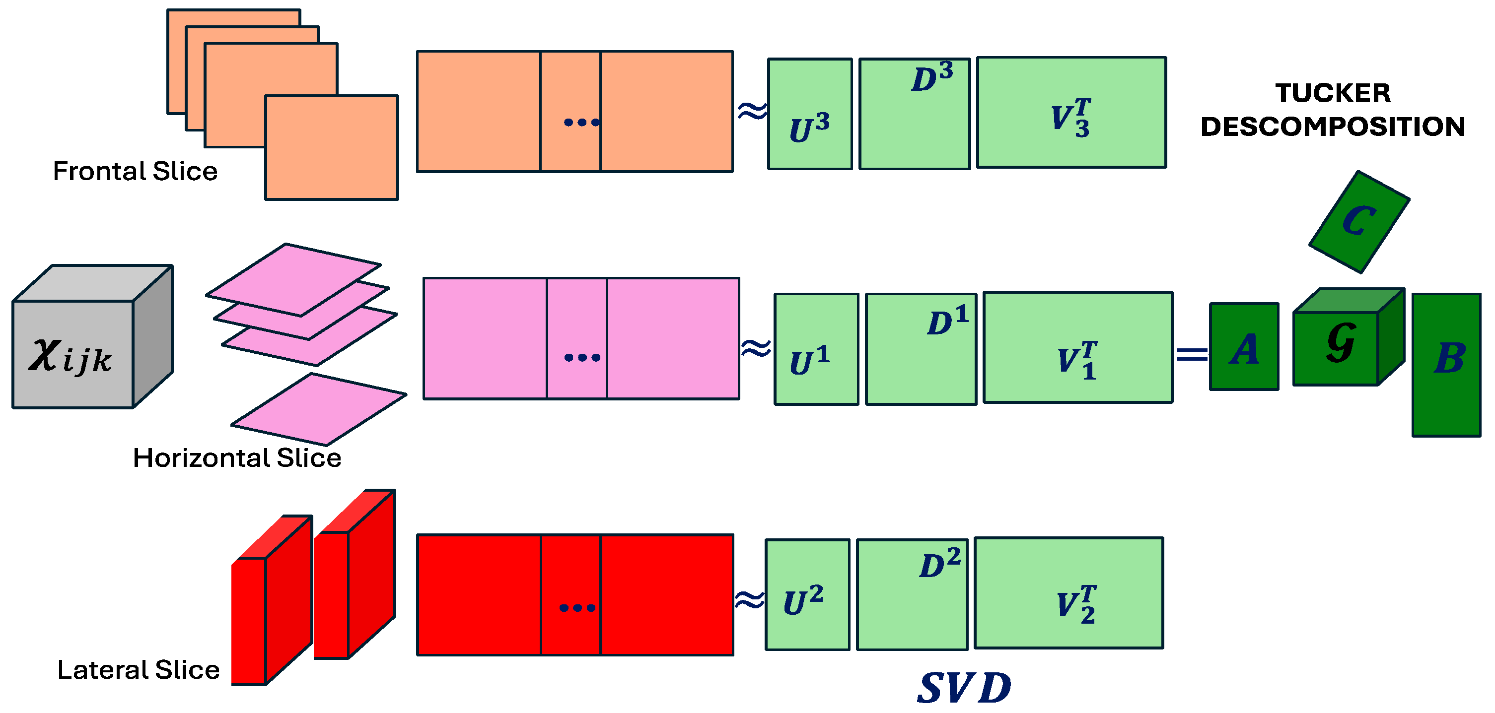
Figure 1 illustrates the Tucker decomposition, where the three-dimensional tensor ${\chi }_{ijk}$ is factored into a core tensor $𝓖$ and three loading matrices $\mathit{A}, \mathit{B}, \mathit{C}$, each corresponding to a specific mode of the tensor. This factorization is constructed using mode-wise matrix products, typically derived from singular value decomposition [16]. The visualization highlights the preservation of the original multiway structure, but also a key limitation: the density of the factor matrices, which hinders the identification of sparse supports in the data.

These limitations have motivated the development of penalized extensions of the Tucker model. In particular, the CenetTucker model, proposed by [4], introduces Elastic Net penalties on the loading matrices, promoting structured sparsity and enhancing stability.

2.1.2. CenetTucker: Mode-Wise Elastic Net Regularization

The CenetTucker model, proposed by [4], extends the classical Tucker decomposition by introducing penalization mechanisms specifically designed to improve interpretability, prevent overfitting, and enhance stability in high-dimensional settings. Its central innovation lies in the incorporation of structured regularization on the loading matrices $\mathit{A}, \mathit{B}, \mathrm{and} \mathit{C}$, through combined ${\mathsf{\ell }}_1$ (Lasso) and ${\mathsf{\ell }}_2$ (Ridge) penalties jointly known as Elastic Net regularization [8], building upon the seminal contributions of [7] and Ridge [17].

Formally, the CenetTucker optimization problem is expressed as:

$$\underset{A,B,C,𝓖}{\min }\left|\right|\mathcal{X}-𝓖{\times }_{1}A{\times }_{2}B{\times }_{3}C{\left|\right|}_F^2+\mathsf{\alpha }\left(\left|\right|A{\left|\right|}_1+\left|\right|B{\left|\right|}_1+\left|\right|C{\left|\right|}_1\right)+\left(\beta |({\left|\right|A\left|\right|}_F^2+{\left|\right|B\left|\right|}_F^2+{\left|\right|C\left|\right|}_F^2)\right)$$

where ${‖·‖}_F$ refers to the Frobenius norm, controlling the overall magnitude of the coefficients, while ${‖·‖}_1$ denotes the ${\mathsf{\ell }}_1$-norm, which promotes sparsity in the solution. The hyperparameter α > 0 regulates the strength of the ${\mathsf{\ell }}_1$ penalty, while β > 0 controls the influence of the ${\mathsf{\ell }}_2$ penalty on the model.

This formulation constitutes a direct generalization of the Elastic Net to tensor factorization. Unlike the classical Tucker model—where loading matrices are dense and fail to distinguish between informative and irrelevant variables —the CenetTucker model induces structured sparsity, allowing zeroed coefficients to reveal relevant supports across tensor modes.

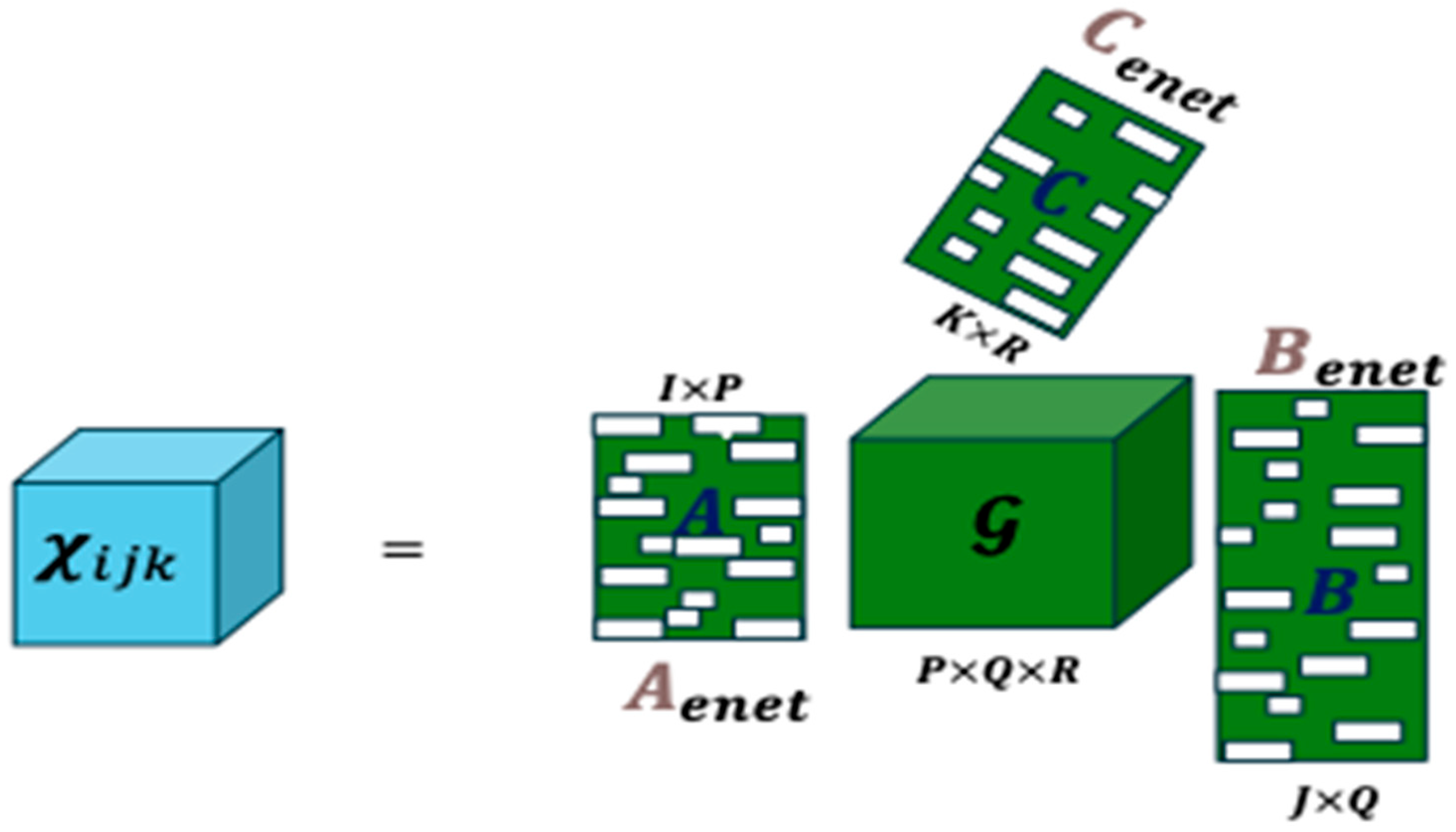
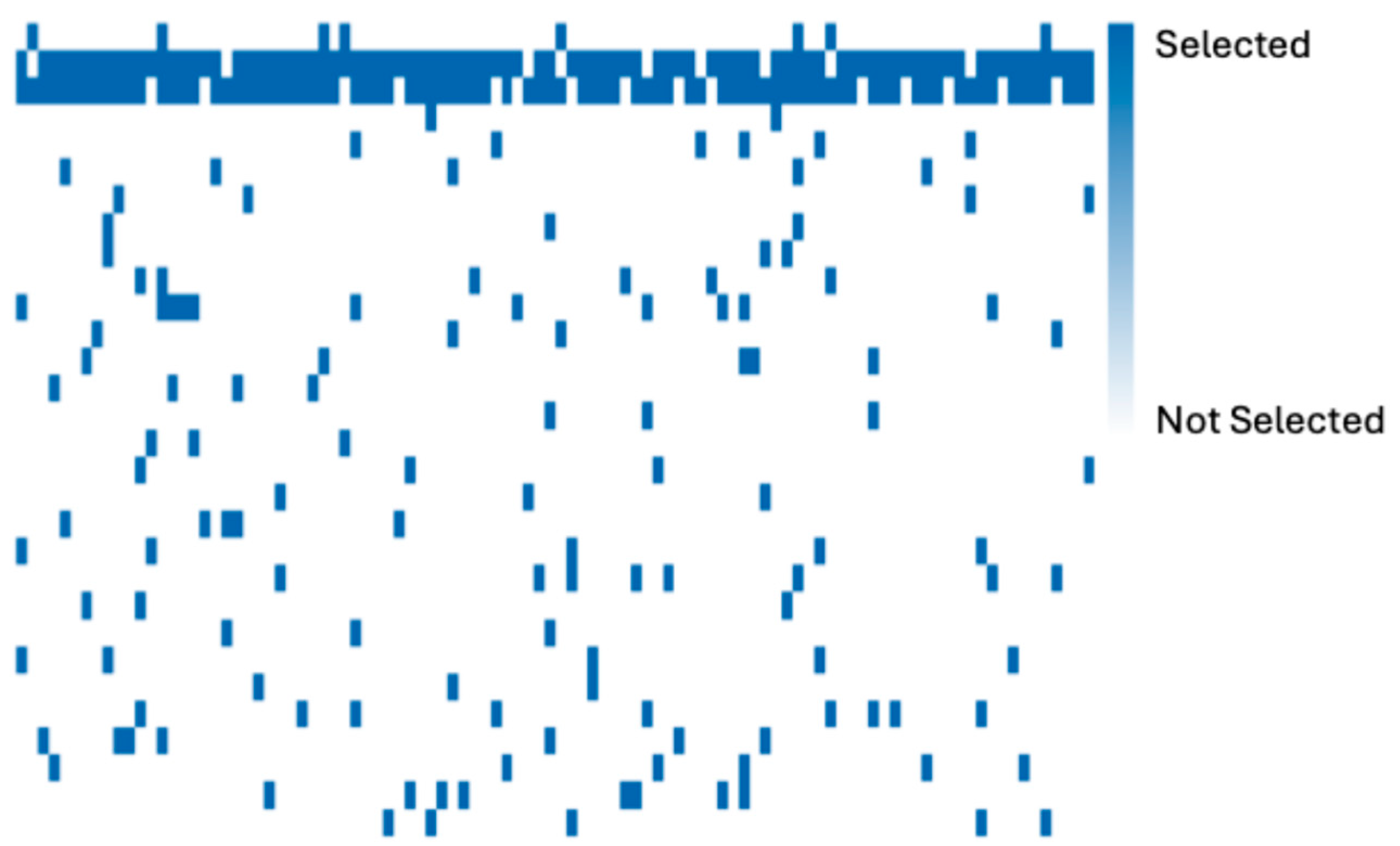
Figure 2 illustrates the decomposition: the tensor ${\mathit{\chi }}_{ijk}$ is approximated by a core tensor $𝓖$ and penalized loading matrices ${\mathit{A}}_{enet}, { \mathit{B}}_{enet}, {\mathit{C}}_{enet}$, obtained through Elastic Net regularization. Blank entries in the matrices indicate coefficients shrunk to zero by the ${\mathsf{\ell }}_1$ penalty, while the non-zero coefficients are smoothed by the ${\mathsf{\ell }}_2$ penalty, ensuring controlled shrinkage and improved stability.

Hyperparameter Selection: α and β

The selection of hyperparameters is performed systematically rather than arbitrarily. González-García (2019) proposes grid search combined with cross-validation procedures (e.g., k-fold or Monte Carlo cross-validation) to identify the optimal pair (α, β). Candidate values are typically chosen on a logarithmic scale (e.g., {10⁻³, 10⁻², …, 1}) to capture different intensities of penalization.

For each candidate pair, the model is fitted on a training set, and its performance is assessed on a validation set using the reconstruction error (Frobenius norm). Depending on the application, domain-specific criteria such as RMSE or correlation with a response variable may also be considered. The pair (α, β) minimizing the average validation error is retained, ensuring a balance between reconstruction accuracy, interpretability, and numerical stability.

Methodological Note: At this stage of the CenetTucker model, the selected hyperparameters are fixed throughout the analysis. They are not recalculated for each sample nor do they vary across resampling iterations. The objective is to determine a global configuration that performs well on the original dataset, optimizing the latent representation of the tensor while avoiding bias from recalibration.

In summary, while the classical Tucker model focuses on minimizing reconstruction error, it often yields dense and unstable solutions. The CenetTucker model overcomes these limitations by introducing Elastic Net regularization, which promotes sparsity and controls coefficient magnitude. This leads to more interpretable and robust decompositions, particularly suitable for high-dimensional contexts.

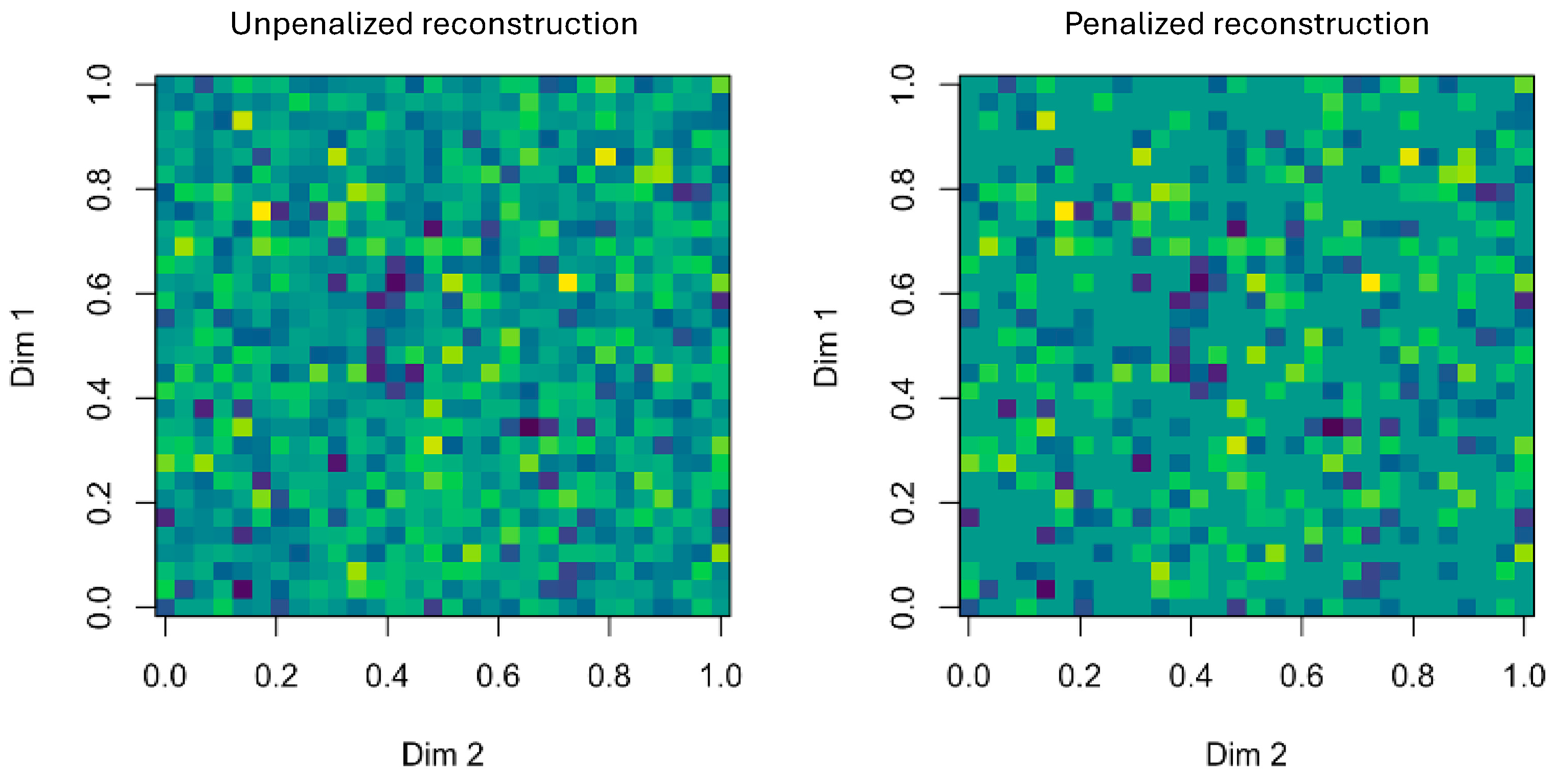
Figure 3 highlights the differences: while the classical Tucker reconstruction (left) appears dense and noisy, the CenetTucker reconstruction (right) reveals clearer and more structured patterns. This enhanced interpretability and stability provide the foundation for the bootstrap-based evaluation of structural stability introduced in the following sections.

2.1.3. BCenetTucker: Bootstrap-Based Assessment of Stability in Penalized Tensor Decompositions

The BCenetTucker method is an original methodological extension designed to evaluate the structural stability of the sparse solutions obtained through the CenetTucker model, particularly in high-dimensional contexts where latent structure identification is highly sensitive to noise and sampling variability.

Motivation: Reproducibility and Structural Robustness in Sparse Models

The core motivation stems from a critical observation: in penalized models that induce sparse solutions, such as CenetTucker, the presence of zero coefficients does not guarantee stability. Solutions with similar reconstruction errors may yield drastically different supports when the input data is slightly perturbed. This fragility raises serious concerns regarding the reproducibility and interpretability of the inferred latent patterns, which are specifically problematic in sensitive applications such as biomarker discovery, neuroimaging, or social segmentation.

To address this issue, the BCenetTucker protocol introduces a structured resampling strategy that generates multiple perturbed versions of the original tensor to study the consistency of active supports under bootstrap variability. Unlike traditional approaches such as Stability Selection [10], BCenetTucker explicitly preserves the tensorial structure and applies a coherent regularization scheme across all resampling iterations, making it more suitable for multiway data.

Overview of the Procedure

The proposed method generates multiple bootstrap replicates of the original tensor by resampling along mode-1 (observations) while preserving the internal structure. For each replicate, the CenetTucker model is fitted using a fixed penalization scheme, and the active supports —defined as rows with non-zero coefficients— are extracted from the factor matrices A, B, and C, as shown in Algorithm 1. The frequency of inclusion of each element across replicates is then used to compute structural stability metrics.

Algorithm 1. General algorithm of the BCenetTucker protocol.
Step	Description
1.	Define the number of bootstrap replicates B and the base CenetTucker model.
2.	Select global hyperparameters (α, β) via cross-validation on the original dataset (see Section 2.3.3).
3.	For each replicate b = 1, …, B  a. Generate a bootstrap sample ${\mathit{X}}^{\left(b\right)}$ by resampling (with replacement) along mode-1 (observations).  b. Fit the CenetTucker model on ${\mathit{X}}^{\left(b\right)}$, using the fixed α and β values.  c. Extract the active supports of ${\mathit{A}}_{enet}, { \mathit{B}}_{enet}, {\mathit{C}}_{enet}$(rows with non-zero coefficients).  d. Store the supports and coefficients for subsequent analysis.
4.	Aggregate the support sets to compute stability metrics by mode (see Section 2.4).
5.	(Optional) Compare against alternative structural validation methods (see Section 2.5).

• Methodological Note on Hyperparameters

In this protocol, the hyperparameters α and β are treated as global. That is, they are selected once via cross-validation on the original dataset and kept fixed across all bootstrap replicates. This methodological decision is grounded in two key principles:

• Structural comparability: Ensuring that any variation in the supports is due to sampling variability, not changes in hyperparameter tuning.
• Bias control: Avoiding resample-specific hyperparameter recalibration, which could introduce noise-induced bias.

The detailed justification for this strategy and its theoretical implications will be addressed in Section 2.3.3.

2.2. Foundations of Bootstrap in Penalized Models

2.2.1. Classical Bootstrap Foundations

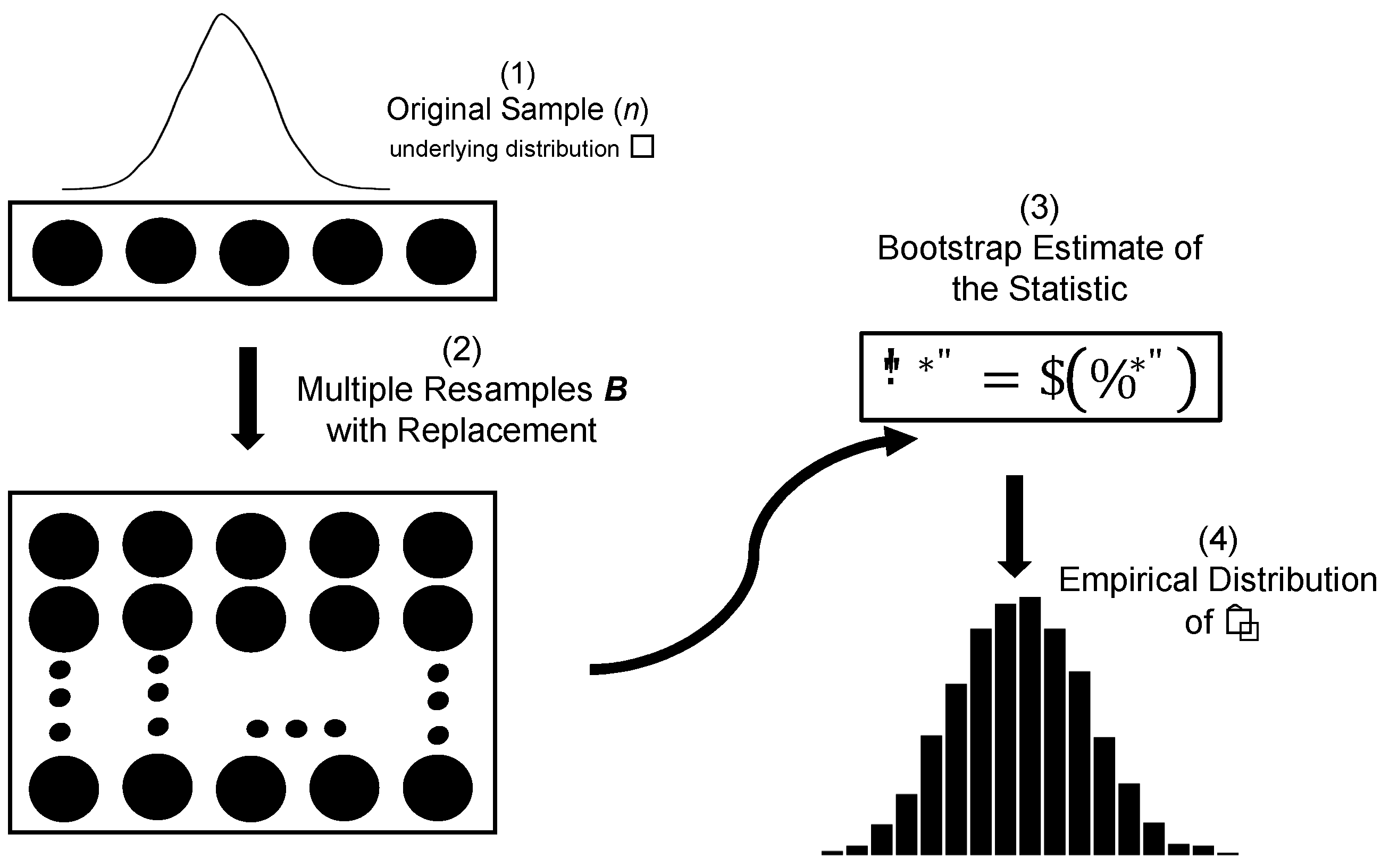
The bootstrap method, originally introduced by [18], stands as one of the most influential tools in modern statistical inference. At its core, the bootstrap relies on generating multiple resampled datasets from the observed data—by resampling with replacement—to approximate the empirical distribution of a statistic without relying on strong parametric assumptions about the population distribution.

Formally, let $𝒳$ = {x₁, …, xₙ} denote an i.i.d. sample drawn from an unknown distribution $\mathbb{F}$. Our goal is to estimate a population parameter θ = t($\mathbb{F}$), such as the mean, variance, regression coefficient, or any other functional of $\mathbb{F}$. Since $\mathbb{F}$ is unobservable, it is replaced by its empirical counterpart, the empirical distribution function ${\widehat{\mathbb{F}}}_{\mathrm{n}}$, which assigns mass 1/n to each observed point. Resampling from ${\widehat{\mathbb{F}}}_{\mathrm{n}}$ yields bootstrap samples that mimic draws from $\mathbb{F}$, thereby enabling inference.

The classical nonparametric bootstrap proceeds as outlined in Algorithm 2.

Algorithm 2. Classical bootstrap procedure.

Algorithm: Non-Parametric Bootstrap

Input: Sample $\mathit{{\rm X}}=\left\{{\mathit{x}}_1,{\mathit{x}}_2, \dots , {\mathit{x}}_{\mathit{n}}\right\}$, number of replications B, statistic of interest $\mathit{t}\left(·\right)$

Output: Empirical distribution of $\widehat{\mathit{\theta }}$, bias estimates, standard error, and confidence intervals.

For  $\mathit{b}=1$ to B, do: 1.  Generate Bootstrap samples ${\mathit{X}}^{\ast \mathit{b}}~{\widehat{\mathit{F}}}_{\mathit{n}}$ by sampling with replacement from the original data of size n. 2.  Compute the Bootstrap statistic: ${\widehat{\mathit{\theta }}}^{\mathit{*}\mathit{b}}=\mathit{t}\left({\mathit{X}}^{\mathit{*}\mathit{b}}\right)$ end for 3.  Compute the empirical distribution $\left\{{\widehat{\mathit{\theta }}}^{\left(1\right)}, \dots , {\widehat{\mathit{\theta }}}^{\left(\mathit{B}\right)}\right\}$ 4.  Compute the Bootstrap mean:${\overline{\mathit{\theta }}}^{\ast }={\displaystyle \frac{1}{\mathit{B}}}\sum _{\mathit{b}=1}^{\mathit{B}}{\widehat{\mathit{\theta }}}^{\ast \mathit{b}}$ 5.  Compute the standard error:${\mathit{S}\mathit{E}}_{\mathit{b}\mathit{o}\mathit{o}\mathit{t}}=\sqrt{{\displaystyle \frac{1}{\mathit{B}-1}}}{\sum }_{\mathit{b}=1}^{\mathit{B}}{\left({\widehat{\mathit{\theta }}}^{\mathit{*}\mathit{b}}-{\overline{\mathit{\theta }}}^{\ast }\right)}^2$ 6.  Estimate the percentile confidence interval: ${\mathit{I}\mathit{C}}_{1-\mathit{\alpha }}=\left[{\widehat{\mathit{\theta }}}_{{\displaystyle \raisebox{1ex}{$\mathit{\alpha }$}\!\left/ \!\raisebox{-1ex}{$2$}\right.}}^{\ast }, {\widehat{\mathit{\theta }}}_{{\displaystyle \raisebox{1ex}{$1-\mathit{\alpha }$}\!\left/ \!\raisebox{-1ex}{$2$}\right.}}^{\ast }\right]$

This method allows for robust estimation of uncertainty in a wide array of settings. Bootstrap confidence intervals (e.g., percentile intervals) and standard error estimates are particularly valuable in complex models where asymptotic approximations are unreliable or unavailable. Furthermore, the bootstrap enables sensitivity analysis, bias correction, model validation, and resampling-based hypothesis testing.

Traditional Applications

The classical bootstrap has found extensive applications in regression models, variance estimations, model diagnostics, survival analysis, and time series modeling, particularly in contexts where analytical solutions are intractable. Standard references include [19,20,21]. Its appeal lies in its minimal assumptions and ease of implementation, even for complex or nonlinear estimators.

Figure 4 provides a schematic illustration of the classical bootstrap workflow, showing the generation of bootstrap samples and the construction of the empirical distribution of the estimator.

2.2.2. Bootstrap in High Dimensionality and Penalization

In penalized models such as Lasso [7] or Elastic net [8], the focus of the bootstrap has shifted from point estimation to the assessment of support stability. This perspective is especially relevant in the presence of structural sparsity. The support of an estimator $\widehat{\beta ,}$ denoted as:

$$supp\left(\widehat{\beta }\right)=\left\{j\in \{1, \dots , p\}:{\widehat{\beta }}_j\ne 0\right\}$$

represents the subset of variables selected by the model and plays a central role in the interpretability and replicability of sparse solutions. In high-dimensional settings, where model complexity and data sparsity coexist, even minor perturbations in the sample can cause significant variability in the support, undermining the reliability of the selection process.

Ref. [9] highlighted this challenge through the Bolasso (bootstrap-enhanced Lasso), demonstrating that the active sets obtained across bootstrap replicates may differ substantially, particularly in the presence of high collinearity or near-zero signal-to-noise ratios. Formally, for bootstrap samples ${\mathit{X}}^{\ast \left(\mathit{b}\right)}$ and ${\mathit{X}}^{\ast \left({\mathit{b}}^{\prime }\right)}$, and their corresponding penalized estimates ${\widehat{\beta }}^{\left(b\right)}$ and ${\widehat{\beta }}^{\left(b^{\prime }\right)}$, one may frequently observe:

$$supp\left({\widehat{\beta }}^{\left(b\right)}\right)\ne supp\left({\widehat{\beta }}^{\left(b^{\prime }\right)}\right)\mathrm{for} \mathrm{two} \mathrm{replicates} b\ne b^{\prime }$$

This phenomenon underscores a fundamental limitation: penalization alone does not guarantee support consistency. The need for an additional validation layer becomes particularly acute in high-dimensional contexts, where traditional asymptotic guarantees are insufficient.

To address this instability, ref. [11] introduced Stability Selection, a methodological innovation that leverages bootstrap resampling to compute empirical selection probabilities for each variable. Letting ${\widehat{\mathit{\pi }}}_{\mathit{j}}$ denote the estimated selection probability for variable $\mathit{j}$, defined as:

$${\widehat{\pi }}_j={\displaystyle \frac{1}{B}}\sum _{b=1}^B\mathbb{I}\left({\widehat{\beta }}_j^{\left(b\right)} \ne 0\right)$$

one can derive a stable support set by thresholding:

$${\widehat{S}}_{stable}=\left\{j:{\widehat{\pi }}_j\ge {\pi }_{thr}\right\}$$

where ${\pi }_{thr}\in \left(0, 1\right)$ is a predefined stability threshold (typically 0.8 or higher).

Importantly, under mild assumptions—such as mutual independence among irrelevant predictors—this framework allows for theoretical control of the Per-Family Error Rate (PFER). Specially, if $q=\mathbb{E}\left[\left|{\widehat{S}}_b\right|\right]$ is the expected number of selected variables per bootstrap replicate, and τ denotes the maximum selection probability of a truly irrelevant variable, then the following inequality holds:

$$PFER\le {\displaystyle \frac{q^2}{2p{\left({\mathit{\pi }}_{\mathit{t}\mathit{h}\mathit{r}}-\mathit{\tau }\right)}^2}}$$

This result establishes, for the first time in this class of procedures, an explicit and interpretable upper bound on the expected number of false inclusions—the Per-Family Error Rate (PFER)—offering a rigorous measure of structural reliability without relying on strong distributional assumptions or multiple-testing corrections.

By integrating bootstrap-based selection frequencies with thresholding rules and error control mechanisms, this class of procedures reframes the bootstrap as a structural validation tool rather than merely a resampling-based inference method. Its relevance has been further supported by empirical work in various domains, including genomics, neuroimaging, and high-dimensional time series [22].

Taken together, these contributions establish a robust framework for evaluating model reproducibility in sparse, high-dimensional environments. The bootstrap, when appropriately embedded within a penalized estimation strategy, emerges not only as a means of statistical estimation but as a pillar for structural certainty and model credibility.

Building on these concepts of support stability and resampling-based validation, we now introduce the BCenetTucker method, which adapts these principles to the tensor decomposition setting.

2.3. The BCenetTucker Method

The BCenetTucker method is introduced as a bootstrap-based framework specifically designed to assess the structural stability of sparse representations derived from the CenetTucker decomposition. Rather than acting as a generic resampling wrapper, BCenetTucker integrates non-parametric resampling with penalized tensor factorization, thereby providing a rigorous structural validation strategy tailored for multiway data. Its primary objective is to quantify the variability of the model′s active structure (support) under perturbations of the original data, offering an empirical measure of the reproducibility of sparse components.

This approach builds upon seminal advances in the stability analysis of penalized models [9,10,11] but adapts them to the tensor domain. In contrast to vector- or matrix-based regularization—where sparsity is imposed on a single set of coefficients—tensor decompositions distribute sparsity across multiple modes, each potentially subject to distinct structural variabilities. Accordingly, the BCenetTucker method extends the classical notions of support and selection stability into a higher-order context.

Formally, let $\mathit{\chi }\in {\mathbb{R}}^{I\times J\times K}$ be a third-order data tensor, where the three modes typically represent subjects, features, and experimental conditions. The procedure generates B bootstrap replicates, ${\mathit{\chi }}^{\left(1\right)}, \cdots , {\mathit{\chi }}^{\left(\mathit{B}\right)}$, each obtained by resampling along the first mode (observational units), while preserving the intrinsic structure along the remaining modes. This resampling scheme ensures that the variability captured by the bootstrap reflects uncertainty in the sampling units without disrupting the multiway organization of the data.

2.3.1. General Procedure Scheme

The BCenetTucker procedure consists of three main steps: (1) generation of bootstrap replicates via mode-1 resampling; (2) penalized tensor factorization using the CenetTucker model on each replicate; and (3) extraction and aggregation of the support for structural stability evaluation.

• Step 1: Generation of bootstrap replicates (mode-1)

Each bootstrap replicate ${\mathit{\chi }}^{\left(\mathit{b}\right)}\in {\mathbb{R}}^{I\times J\times K}$ is generated by resampling with replacement along the first mode (observational units), while keeping mode-2 and -3 fixed. Specifically, the index set {1, …, I} is resampled to procedure a sequence $i_b\left(I\right), \cdots , i_b\left(I\right)$ where repetions are allowed. Formally:

$${\mathit{\chi }}^{\left(\mathit{b}\right)}={\left\{{\mathit{\chi }}_{{\mathit{i}}_{\mathit{b}}\left(\mathit{j}\right),:,:}\right\}}_{\mathit{j}=1}^{\mathit{I}},\hspace{1em}\mathrm{where} {\mathit{i}}_{\mathit{b}}\left(\mathit{j}\right)\sim \mathrm{Unif}\{\mathbf{1}, \dots , \mathit{I}\}$$

Mode-1 resampling is particularly appropriate when mode-1 corresponds to observational units, as it preserves the intrinsic structure of experimental variables and conditions. This resampling strategy allows mode-1 to contain duplicated slices, thereby capturing the stochastic variability in the population of observational units. In contrast, mode-2 and -3 remain unaltered, preserving the multiway correlation structure that is essential for meaningful tensor decomposition. Similar mode-specific resampling schemes have been adopted in tensor regression contexts [5,23], highlighting the importance of maintaining inter-mode dependencies during the resampling process.

• Step 2: Penalized CenetTucker estimation

For each bootstrap replicate ${\mathit{\chi }}^{\left(b\right)}$, the CenetTucker model is estimated using a fixed Elastic Net regularization scheme. This hybrid regularization is applied to the mode-specific loading matrices ${\mathit{A}}^{\left(\mathit{b}\right)}, {\mathit{B}}^{\left(\mathit{b}\right)}, {\mathit{C}}^{\left(\mathit{b}\right)}$ while the tensor core ${𝓖}^{\left(\mathit{b}\right)}$ captures the low-rank interactions across modes. The penalized model minimizes the objective:

$$\begin{gathered} \underset{{𝓖}^{\left(\mathrm{b}\right)},\hspace{0.17em}{A}^{\left(b\right)},\hspace{0.17em}{B}^{\left(b\right)},\hspace{0.17em}{C}^{\left(b\right)}}{\mathrm{m}\mathrm{i}\mathrm{n}}\left|\right|{\chi }^{\left(b\right)}-{𝓖}^{\left(b\right)}{\times }_1{A}^{\left(b\right)}{\times }_2{B}^{\left(b\right)}{\times }_3{C}^{\left(b\right)}{\left|\right|}_F^2+\alpha \left(\left|\right|A^{\left(b\right)}{\left|\right|}_1+\left|\right|B^{\left(b\right)}{\left|\right|}_1+\left|\right|C^{\left(b\right)}{\left|\right|}_1\right) \\ +\beta \left(\left|\right|A^{\left(b\right)}|{|}_F^2+|\left|B^{\left(b\right)}\right|{|}_F^2+\left|\right|C^{\left(b\right)}|{|}_F^2\right) \end{gathered}$$

Here, the ${\mathsf{\ell }}_1$ promotes sparsity by encouraging zero coefficients, while the ${\mathsf{\ell }}_2$ norm provides numerical stability and discourages overfitting. The simultaneous use of both penalties, characteristic of Elastic Net regularization, has shown superior performance in high-dimensional scenarios by mitigating multicollinearity while preserving interpretability.

• Step 3: Bootstrap support extraction

Once the penalized model is fitted, the active set—or support—is extracted from each loading matrix by identifying rows with at least one non-zero coefficient. This yields three support sets per replicate: ${\mathit{S}}_{\mathit{b}}^{\mathit{A}}$, ${\mathit{S}}_{\mathit{b}}^{\mathit{B}}$, ${\mathit{S}}_{\mathit{b}}^{\mathit{C}}$, corresponding to the observational, variable, and conditions modes, respectively. Formally:

$$\begin{gathered} \mathit{s}\mathit{u}\mathit{p}\mathit{p}\left({\mathit{A}}^{\left(\mathit{b}\right)}\right)=\left\{\mathit{i}\in \{\mathbf{0}, \dots , \mathit{I}\}:||{\mathit{A}}_{\mathit{i},\cdot }^{\left(\mathit{b}\right)}{\left|\right|}_{\mathbf{0}}>\mathbf{0}\right\} \\ \mathit{s}\mathit{u}\mathit{p}\mathit{p}\left({\mathit{B}}^{\left(\mathit{b}\right)}\right)=\left\{\mathit{j}\in \{\mathbf{0}, \dots , \mathit{J}\}:||{\mathit{B}}_{\mathit{j},\cdot }^{\left(\mathit{b}\right)}{\left|\right|}_{\mathbf{0}}>\mathbf{0}\right\} \\ \mathit{s}\mathit{u}\mathit{p}\mathit{p}\left({\mathit{C}}^{\left(\mathit{b}\right)}\right)=\left\{\mathit{k}\in \{\mathbf{0}, \dots , \mathit{K}\}:||{\mathit{C}}_{\mathit{k},\cdot }^{\left(\mathit{b}\right)}{\left|\right|}_{\mathbf{0}}>\mathbf{0}\right\} \end{gathered}$$

These supports reflect the empirical selection behavior of the model across perturbations, laying the foundation for assessing selection stability in the subsequent analysis.

2.3.2. Support Extraction in Each Bootstrap Replicate

The extraction of the support structure in each bootstrap replicate constitutes a core component of the BCenetTucker methodology. Given the penalized decomposition of the bootstrap-resampled tensor ${\mathit{\chi }}^{\left(\mathit{b}\right)}$, the aim is to identify the active components that define the sparse representation recovered by the model under data perturbations.

Formally, for each replicate b = 1, …, B, the CenetTucker model is estimated to obtain the regularized mode-specific loading matrices $\mathit{A}\in {\mathbb{R}}^{I\times R_1}, \mathit{B}\in {\mathbb{R}}^{J\times R_2}, \mathit{C}\in {\mathbb{R}}^{K\times R_3}$ along with the corresponding core tensor ${𝓖}^{\left(b\right)}$. These objects satisfy the penalized approximation:

$${\widehat{\mathit{\chi }}}^{\left(b\right)}={𝓖}^{\left(b\right)}{\times }_1{\mathit{A}}^{\left(b\right)}{\times }_2{\mathit{B}}^{\left(b\right)}{\times }_3{\mathit{C}}^{\left(b\right)}$$

where the decomposition is obtained by minimizing a penalized loss function incorporating both ${\mathsf{\ell }}_1$ and ${\mathsf{\ell }}_2$ norms to enforce sparsity and numerical regularization [5].

The notion of support refers to the identification of “active” rows in each loading matrix—that is, those rows that contain at least one non-zero coefficient and thus contribute to the latent factorization. Letting ${‖·‖}_F$ denote the row-wise ${\mathsf{\ell }}_0$-pseudo-norm, the supports are defined as:

$$\begin{gathered} \mathit{s}\mathit{u}\mathit{p}\mathit{p}\left({\mathit{A}}^{\left(\mathit{b}\right)}\right)=\left\{\mathit{i}\in \{\mathbf{0},\dots ,\mathit{I}\}:||{\mathit{A}}_{\mathit{i},\cdot }^{\left(\mathit{b}\right)}{\left|\right|}_{\mathbf{0}}>\mathbf{0}\right\} \\ \mathit{s}\mathit{u}\mathit{p}\mathit{p}\left({\mathit{B}}^{\left(\mathit{b}\right)}\right)=\left\{\mathit{j}\in \{\mathbf{0},\dots ,\mathit{J}\}:\left|\right|{\mathit{B}}_{\mathit{j},\cdot }^{\left(\mathit{b}\right)}{\left|\right|}_{\mathbf{0}}>\mathbf{0}\right\}, \\ \mathit{s}\mathit{u}\mathit{p}\mathit{p}\left({\mathit{C}}^{\left(\mathit{b}\right)}\right)=\left\{\mathit{k}\in \{\mathbf{0},\dots ,\mathit{K}\}:\left|\right|{\mathit{C}}_{\mathit{k},\cdot }^{\left(\mathit{b}\right)}{\left|\right|}_{\mathbf{0}}>\mathbf{0}\right\}, \end{gathered}$$

These sets of indices identify the features, conditions, or observational units (depending on the mode) that are actively engaged in shaping the model′s latent structure in replicate b. This structural interpretation aligns with the geometric notion of sparsity in high-dimensional models [23], where inactive rows (i.e., those consisting entirely of zeros) are effectively excluded from the representation.

By collecting the extracted supports across all bootstrap replicates, one obtains three mode-specific support ensembles:

$$\begin{gathered} {𝓢}^{\mathit{A}}={\left\{\mathit{s}\mathit{u}\mathit{p}\mathit{p}\left({\mathit{A}}^{\left(\mathit{b}\right)}\right)\right\}}_{\mathit{b}=1}^{\mathit{B}} \\ {{𝓢}^{\mathit{B}}=\left\{\mathit{s}\mathit{u}\mathit{p}\mathit{p}\left({\mathit{B}}^{\left(\mathit{b}\right)}\right)\right\}}_{\mathit{b}=1}^{\mathit{B}} \\ {𝓢}^{\mathit{C}}={\left\{\mathit{s}\mathit{u}\mathit{p}\mathit{p}\left({\mathit{C}}^{\left(\mathit{b}\right)}\right)\right\}}_{\mathit{b}=1}^{\mathit{B}} \end{gathered}$$

These collections serve as the empirical basis for assessing structural stability. Their analysis, through frequency-based and similarity metrics, allows for a quantitative evaluation of how consistently specific rows (i.e., features, conditions, subjects) are selected across perturbations of the data distribution. Such assessment is crucial in high-dimensional settings, where small fluctuations in the data can significantly alter the selected support [10,11].

This framework establishes a robust foundation for measuring the reproducibility of sparse structures identified by the penalized decomposition and directly connects with the broader literature on Stability Selection and support uncertainty in modern statistical learning.

2.3.3. Selection of Hyperparameters $\mathit{\alpha } \mathrm{and} \mathit{\beta }$ in BCenetTucker

The BCenetTucker method employs Elastic Net regularization, which involves two critical hyperparameters: $\alpha$, controlling the overall penalty strength, and $\beta$, determining the balance between ${\mathsf{\ell }}_1$ (Lasso) and ${\mathsf{\ell }}_2$ (Ridge) components. A central methodological decision lies in whether to recalibrate these parameters within each bootstrap replicate or to fix them across all resampled tensors.

Fixed Hyperparameters Across Replicates

In this study, both $\mathit{\alpha }$ and $\mathit{\beta }$ are fixed prior to the bootstrap and applied identically across all B replicates. This decision is grounded in both practical and theoretical considerations:

Comparability and interpretability: Maintaining constant penalization parameters ensures that variability in support selection across replicates is solely attributable to data perturbations, rather than fluctuations in the penalization scheme. This design facilitates a direct and unbiased assessment of structural stability.

Avoidance of overfitting within replicates: Re-estimating hyperparameters within each bootstrap sample could induce selection noise and inflate the support variability, undermining the reproducibility goals for the method.

Theoretical precedent

Similar strategies have been employed in the context of Stability [10,11], where fixed regularization paths are essential to ensure coherence of variable selection frequencies across resamples.

• Hyperparameter Calibration via Cross-Validation

The selection of the regularization parameters $\left(\alpha , \beta \right)$ plays a central role in the behavior of the CenetTucker model. In the BCenetTucker framework, this calibration can be approached in different ways, depending on the specific objective of the analysis.

In this implementation, we adopt a fixed hyperparameter approach. Before bootstrap resampling, a grid search over candidate values $\left(\alpha , \beta \right)\in \mathcal{A}\times \mathcal{B}$ is conducted on the original dataset. Ten-fold cross-validation is used to select the optimal pair $\left({\alpha }^{*}, {\beta }^{*}\right)$ that minimizes the penalized reconstruction error:

$$\mathit{C}\mathit{V}\left(\mathit{\alpha },\mathit{\beta }\right)={\displaystyle \frac{1}{\mathit{K}}}\sum _{\mathit{k}=1}^{\mathit{K}}{‖{\mathit{\chi }}^{\left(\mathit{k}\right)}-{𝓖}^{\left(\mathit{k}\right)}{\times }_{\mathbf{1}}{\mathit{A}}^{\left(\mathit{k}\right)}{\times }_{\mathbf{2}}{\mathit{B}}^{\left(\mathit{k}\right)}{\times }_{\mathbf{3}}{\mathit{C}}^{\left(\mathit{k}\right)}‖}_{\mathit{F}}^{\mathbf{2}}$$

The selected pair $\left({\alpha }^{*}, {\beta }^{*}\right)$ is then held fixed and applied consistently across all bootstrap replicates. This decision is made to ensure comparability between bootstrap estimates and to prevent instability or overfitting introduced by re-optimizing the penalty for each resampled dataset.

• A Flexible and Justifiable Choice

It is important to emphasize that this calibration approach is not a normative requirement. One may instead recalibrate (α, β) within each bootstrap replicate if the goal is to explore sensitivity to regularization strength or if hyperparameter inference itself is of interest. Such a choice should be made deliberately and supported by a clear rationale and implementation design.

The strategy adopted here reflects the specific aim of isolating the variability in the structural support induced by data perturbations—rather than conflating it with changes in model tuning.

Future extensions could explore adaptive tuning of (α, β) based on resampling stability criteria or incorporate Bayesian strategies for uncertainty quantification over regularization paths.

2.4. Structural Stability Metrics by Mode

In the context of high-dimensional penalized tensor decompositions, assessing the structural stability of the estimated supports becomes essential. Traditional reconstruction-focused evaluations overlook a crucial dimension: how reproducible the extracted latent structure is under perturbations to the data. To address this gap, the BCenetTucker framework introduces a set of dedicated metrics specifically designed to quantify support consistency across resampling iterations.

Although some of these metrics are inspired by principles previously established in Stability Selection [10,11] their formulation and adaptation to the tensorial context with multimode penalization constitute a methodological contribution of this work. Specifically, the integration of these metrics within the BcenetTucker resampling and penalization scheme allows for a structurally coherent interpretation that is novel in multiway contexts.

The metrics presented in this section are not generic tools borrowed from classical statistics; rather, they are methodological innovations proposed as part of BcenetTucker. Their objective is to evaluate how frequently and coherently specific tensor elements are selected, filtered, and retained throughout the penalization process applied to multiple bootstrap replicates.

Each metric responds to a complementary aspect of structural stability:

• Inclusion Frequency captures how often individual elements are selected.
• The Average Jaccard Index measures the overall similarity between supports across replicates.
• Stable Selection Index (SSI) identifies the subset of highly reliable selections.
• Proportion of Stable Support allows for cross-mode comparisons normalized by dimensionality.
• Standard Deviation of Support Size quantifies the variability in the number of selected elements.

To enhance interpretability, these metrics are reported separately for each tensor mode. Mode A (observations), Mode B (variables), and Mode C (conditions) are clearly labeled throughout the analysis to differentiate structural behaviors. Where applicable, summary tables consolidate the metrics per mode for comparative visualization.

These metrics enable a transition from point estimates to distributional characterizations of structure. They represent a rigorous, multi-angle strategy to assess robustness, helping distinguish between core signals and unstable artifacts introduced by noise or model tuning. Importantly, they move penalized tensor models closer to reproducible science, offering interpretable summaries that transcend mere numerical fit.

Methodological Note: The decision to use Elastic Net penalization is motivated by its ability to combine the sparsity of LASSO with the stability of Ridge, especially beneficial in contexts with collinearity and high dimensionality. The threshold π_thr = 0.8 for the Stable Selection Index (SSI) follows established practice in the literature to indicate high confidence selections [10]. Additionally, resampling is conducted along mode-1 (observations) to preserve the dependency structures along mode-2 and -3, which are essential for interpreting the tensor′s latent structure.

The following subsections introduce each metric in detail, illustrating their computation, interpretation, and empirical behavior.

2.4.1. Inclusion Frequency

The first metric proposed to assess the structural stability of the penalized model is the inclusion frequency, which empirically estimates the probability that each row of the loading matrices is selected as part of the sparse support in the resampling process. The use of inclusion frequency as an empirical stability metric has been widely promoted within the framework of Stability Selection [10,11], as well as in bootstrap-based variants such as Bolasso [9].

Let $B$ be the number of bootstrap replicates generated and let $S_b^A\subseteq \left\{1, \dots , {\rm I}\right\}$ be the estimated support for mode-1 in replicate $b$, that is, the set of active rows in $A^{\left(b\right)}$. Then, the inclusion frequency for index $i\in \left\{1, \dots , {\rm I}\right\}$ is defined as:

$${\widehat{\Pi }}_i^A={\displaystyle \frac{1}{B}}\sum _{b=1}^B\mathbb{I}\left(i\in S_b^A\right)$$

Analogously, the frequencies for modes B and C are defined as:

$${\widehat{\Pi }}_i^B={\displaystyle \frac{1}{B}}{\sum }_{b=1}^{B}I\left(j\in S_b^B\right) {\widehat{\Pi }}_i^C={\displaystyle \frac{1}{B}}{\sum }_{b=1}^{B}I\left(k\in S_b^C\right)$$

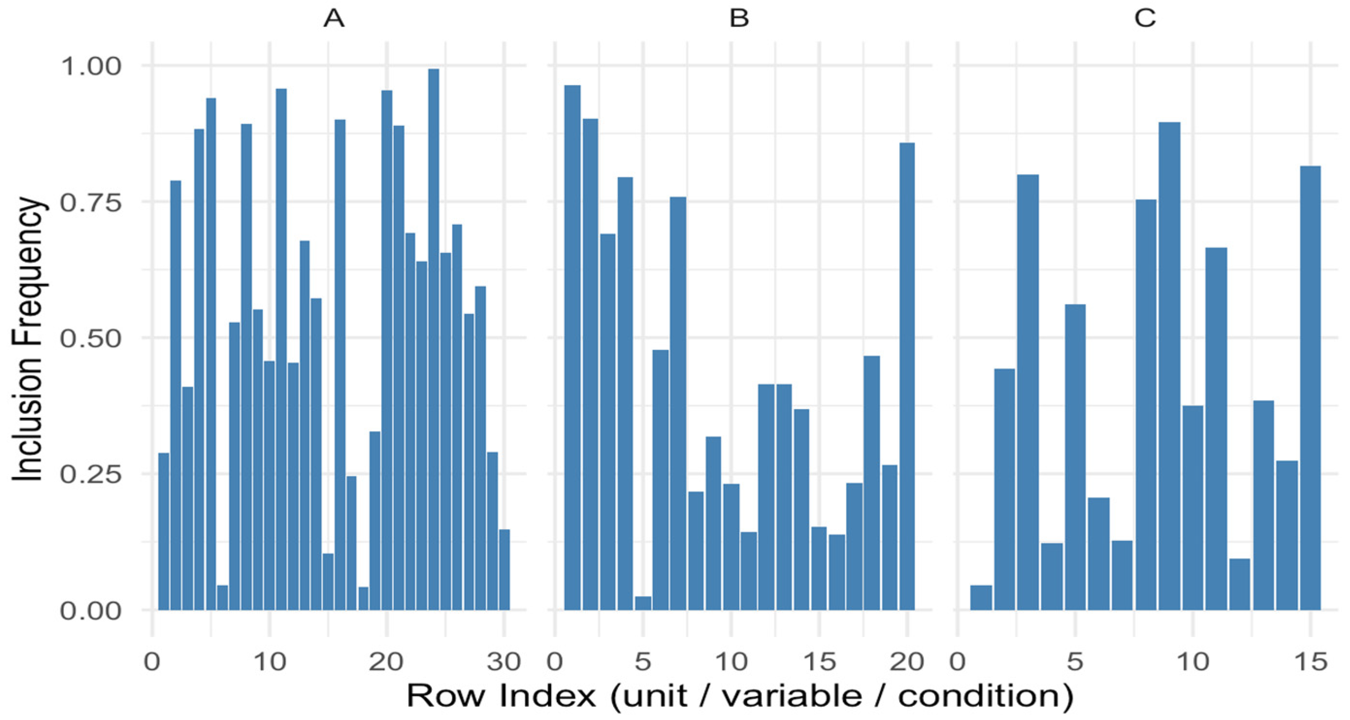
Each inclusion frequency can be interpreted as an empirical estimate of the structural relevance of a given element. Values close to 1 indicate high stability and repeated selection, while values close to 0 suggest inconsistency and low reliability.

Inclusion frequency supports several forms of quantitative interpretation:

(i)

Overall average frequency: Estimates the mean level of inclusion per mode:

$$\widehat{\Pi }={\displaystyle \frac{1}{I}}{\sum }_{i=1}^I{\widehat{\Pi }}_i$$

(ii)

Proportion of rows with high or low inclusion: Quantifies how many rows have ${\widehat{\Pi }}_i\ge 0.8$(high stability) or ${\widehat{\Pi }}_i\ge 0.2$ (high instability) to assess structural concentration or dispersion.

(iii)

Dispersion of frequencies (variance): Can be computed as:

$${\sigma }_{\Pi }^2={\displaystyle \frac{1}{I}}\sum _{i=1}^I{\left(\widehat{{\Pi }_i}-\overline{\Pi }\right)}^2$$

which indicates how homogeneous or dispersed the selection is within each mode.

(iv)

Cross-mode comparison: By analyzing the frequency patterns in each mode, one can identify where the penalized model exhibits greater stability. For instance, if mode $C$ shows a higher concentration of values near 1 compared to $A$ or $B$, this suggests that the latent structure in that mode is more robust or less sensitive to resampling.

These interpretations offer both local and global insights into model behavior and are especially powerful when combined with visualizations such as bar plots.

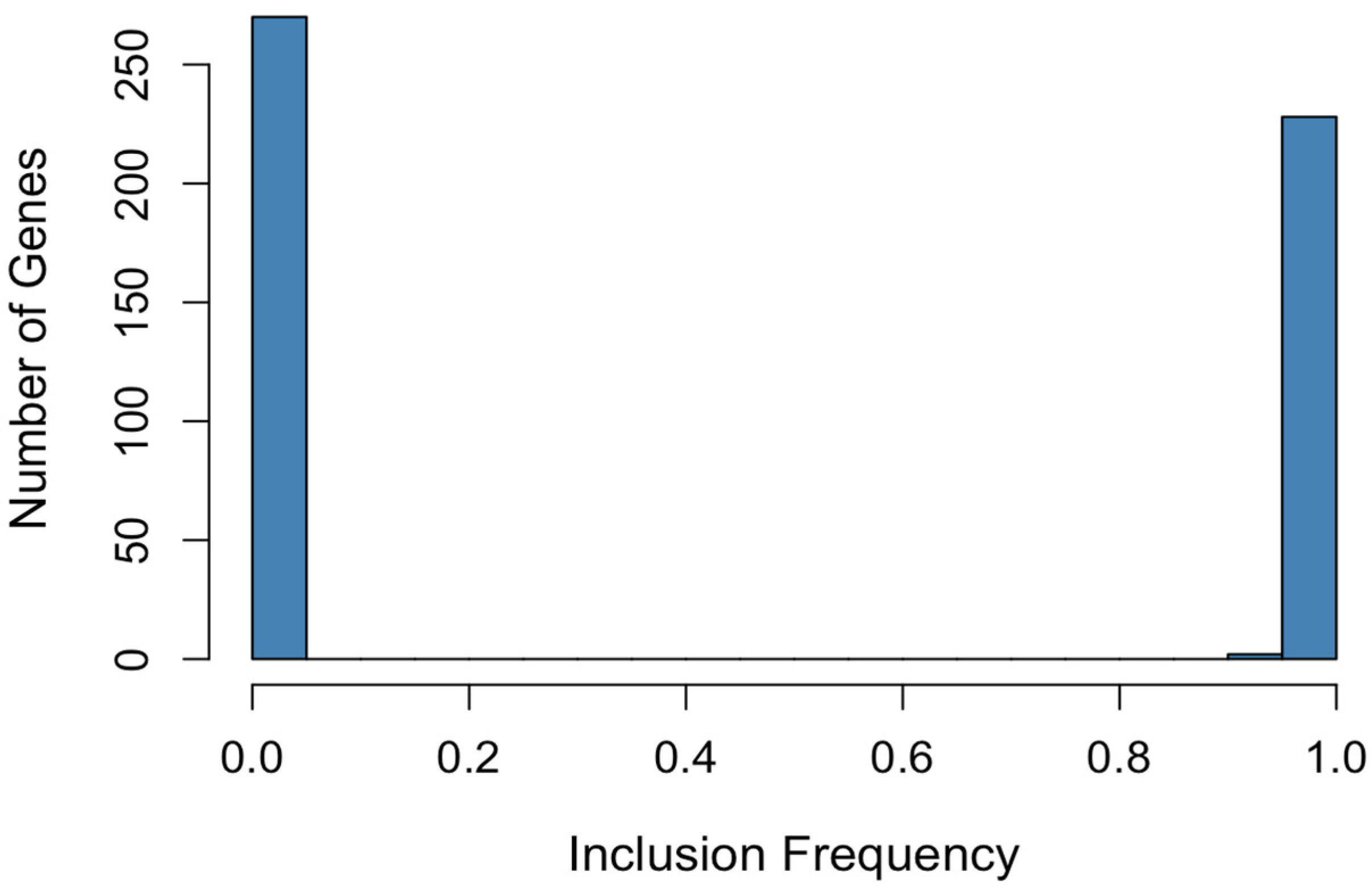
Figure 5 illustrates this metric by displaying the inclusion frequency of each row across bootstrap replicates for all three modes. The height of each bar represents the empirical selection probability for that element. Bars approaching a height of 1 indicate elements that are consistently included, whereas those closer to 0 represent unstable or noise-driven selections. This figure allows a visual inspection of which modes—and which specific indices—contribute more robustly to the structure extracted by the penalized model.

2.4.2. Average Jaccard Index

The average Jaccard index is a classical measure of similarity between sets and is particularly useful in the context of penalized models with resampling, where the goal is to evaluate the structural consistency of the estimated support across different replicates.

Originally formulated by Jaccard (1901), this metric has been widely adopted in statistical learning contexts to assess the stability of variable selection [10,11]. The average Jaccard index provides a global measure of structural stability by comparing the overall similarity between support sets across bootstrap replicates. Unlike inclusion frequency, which focuses on the selection probability of individual elements, the Jaccard index evaluates the coherence of the entire selected structure.

Formally, for any two bootstrap replicates $b$ and $b^{\prime }$, the Jaccard similarity between their estimated support sets $S_b$ and $S_{b^{\prime }}$ is given by:

$$\mathit{J}\left({\mathit{S}}_{\mathit{b}},{\mathit{S}}_{{\mathit{b}}^{\prime }}\right)={\displaystyle \frac{\left|{\mathit{S}}_{\mathit{b}}, {\mathit{S}}_{{\mathit{b}}^{\prime }}\right|}{\left|{\mathit{S}}_{\mathit{b}}\cup {\mathit{S}}_{{\mathit{b}}^{\prime }}\right|}}$$

where $S_b$ and $S_{b^{\prime }}$ are the sets of indices selected as supports in bootstrap replicate $b$ and $b^{\prime }$, respectively.

This index ranges from 0 (no overlap) to 1 (perfect overlap). When extended to all $\left({\displaystyle \genfrac{}{}{0pt}{}{B}{2}}\right)$ pairs of bootstrap replicates for a given mode, the average Jaccard index for a given mode (e.g., mode-A) is defined as:

$${\mathit{J}}_{\mathbf{avg}}^{\mathit{A}}={\displaystyle \frac{2}{\mathit{B}\left(\mathit{B}-1\right)}}\sum _{1\le \mathit{b}<{\mathit{b}}^{\prime }\le \mathit{B}}{\displaystyle \frac{\left|{\mathit{S}}_{\mathit{b}}^{\mathit{A}}\cap {\mathit{S}}_{{\mathit{b}}^{\prime }}^{\mathit{A}}\right|}{\left|{\mathit{S}}_{\mathit{b}}^{\mathit{A}}\cup {\mathit{S}}_{{\mathit{b}}^{\prime }}^{\mathit{A}}\right|}}$$

High values of ${\mathit{J}}_{\mathbf{avg}}^{\mathit{A}}$ (close to 1) indicate that the supports selected across replicates are structurally consistent, while low values (close to 0) reveal high variability in the configuration of selected components.

This metric is particularly valuable when assessing whether the penalized model tends to converge toward a stable latent structure or, conversely, fluctuates between multiple configurations due to noise, collinearity, or a permissive regularization path. It is especially informative in identifying problematic modes where stability is not guaranteed.

This index complements inclusion frequency: while the latter assesses stability row by row, the Jaccard index does so set by set, allowing the capture of aggregate-level structural similarity.

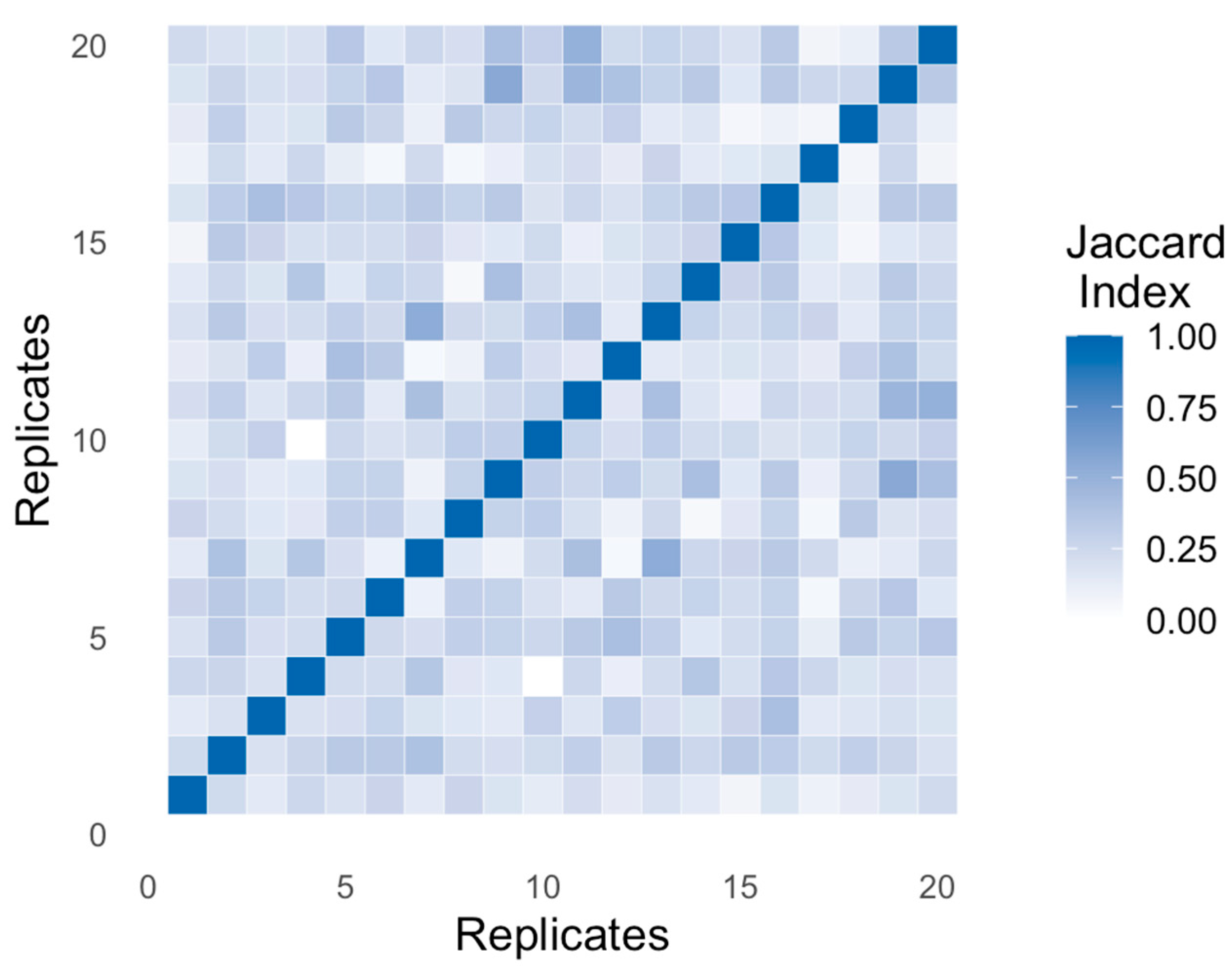
To visualize this behavior, we compute all pairwise Jaccard indices across the B bootstrap replicates and summarize them in a symmetric matrix. This representation offers an intuitive view of structural coherence across resamples and helps reveal potential instability zones in the support configuration.

Figure 6 displays a heatmap of pairwise Jaccard indices across all B bootstrap replicates. As expected, diagonal values are 1, representing perfect self-similarity. Off-diagonal entries reveal how similar different support sets are. A tight concentration of values near 1 suggests robust structural agreement. In contrast, dispersion across the matrix—e.g., values ranging from 0.2 to 0.6—indicates partial or inconsistent selection, which may undermine reproducibility.

This form of global stability assessment complements inclusion frequency, providing a two-level view: one at the element-wise scale, and another at the configuration level.

Methodological note: While Figure 6 is based on simulated data, similar patterns are often observed in high-dimensional settings. In real applications, the average Jaccard index is computed separately for each mode $\left(\mathrm{e}.\mathrm{g}., J_{avg}^A , J_{avg}^B, J_{avg}^C\right)$ and can be used to compare the robustness of structural patterns across modes or to inform thresholding strategies and regularization tuning.

2.4.3. Stable Selection Index (SSI)

Beyond evaluating local stability through inclusion frequency and global coherence via the Jaccard index, it is essential to quantify how many elements exhibit genuinely stable selection across bootstrap replicates. The Stable Selection Index (SSI) addresses this need by computing the number of tensor rows whose inclusion frequency exceeds a predefined stability threshold πthr, thereby identifying the subset of support that can be considered empirically reliable.

The SSI builds upon the framework of Stability Selection introduced by [10] within the framework of Stability Selection and later adapted by [11], adapting its logic to the context of sparse tensor decompositions under multimodal penalization.

Formally, the SSI for mode A is defined as:

$${\mathrm{SSI}}^A=|\{i\in \{1, \dots , I\}:{\widehat{\Pi }}_i^A\ge {\pi }_{\mathrm{thr}}\}|$$

where ${\widehat{\Pi }}_i^A$ denotes the inclusion frequency of row iii in mode A. Analogous formulations apply for modes B and C, yielding ${\mathit{SSI}}^B$ and ${\mathit{SSI}}^C$, respectively.

The threshold ${\pi }_{thr}$ serves as a stability cutoff, commonly set at 0.75 or 0.80 based on theoretical guarantees and empirical conventions [10,11]. However, the specific value can be adjusted depending on dimensionality, signal strength, or the desired trade-off between false positives and interpretability.

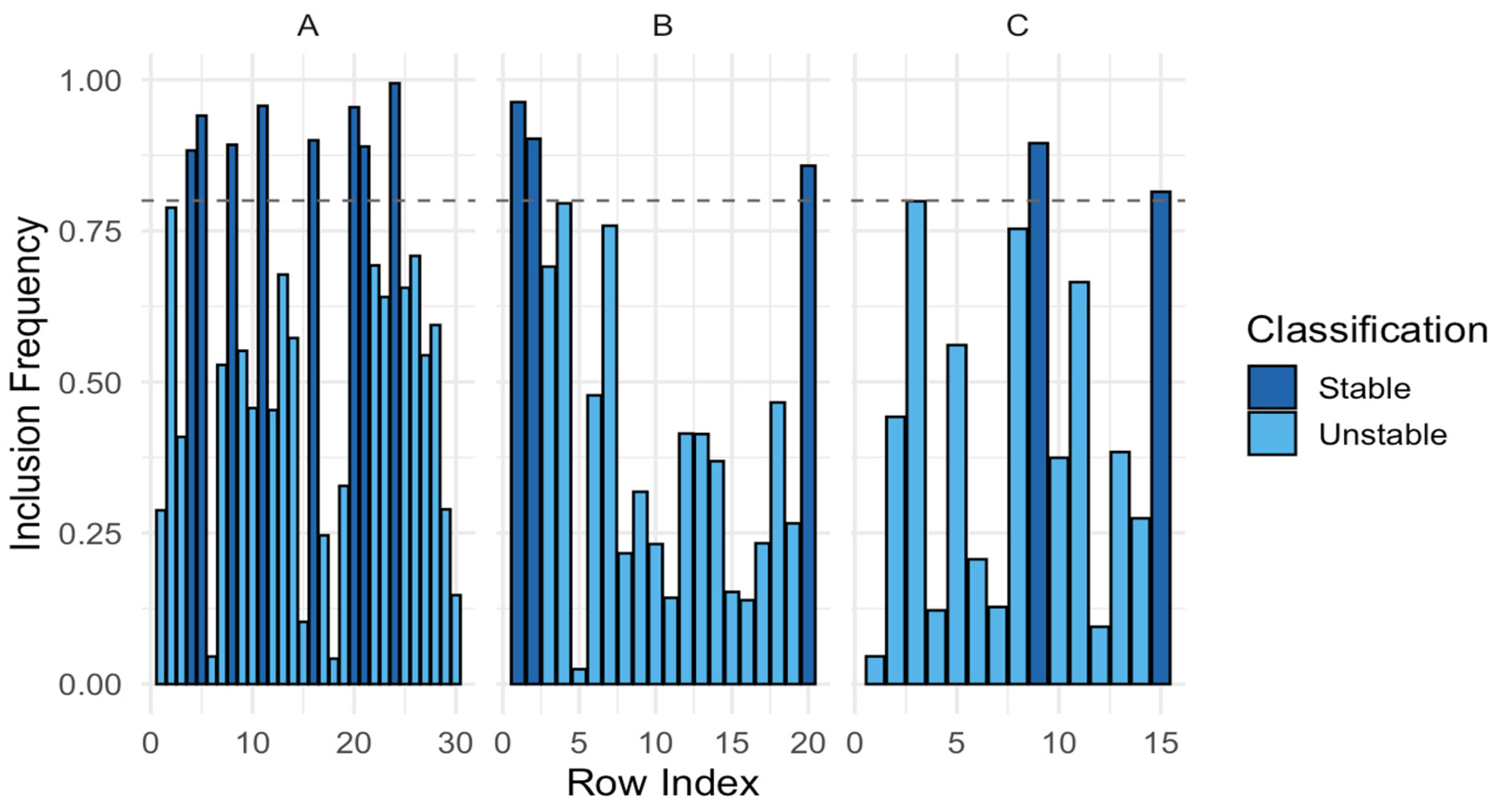
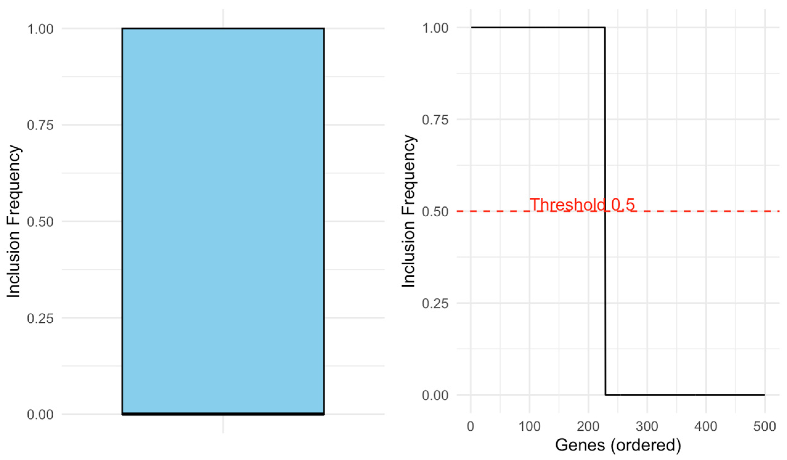
As shown in the Figure 7, Inclusion frequency plots across all tensor modes with classification of stable (dark blue) and unstable (light blue) selections. The dashed horizontal line represents the stability threshold (Π_thr = 0.8).

(A)

Mode A (genes): rows with inclusion frequency ≥ 0.8 are classified as stable gene selections.

(B)

Mode B (samples): rows corresponding to patient samples, showing more variability and a smaller subset of stable supports.

(C)

Mode C (groups): rows representing diagnostic categories (ALL, AML, CML), with clear separation of stable versus unstable components.

2.4.4. Proportion of Stable Support

While the Stable Selection Index (SSI) provides the absolute number of reliably selected elements per mode, it is equally important to express this value in relative terms.

The proportion of stable support offers a normalized view by accounting for the total number of rows in each mode, thus enabling meaningful comparisons across modes with different dimensionalities:

$$\begin{gathered} \mathrm{Stable} {\mathrm{Proportion}}^{ A}={\displaystyle \frac{{\mathit{SSI}}^A}{I}} \\ \mathrm{Stable} {\mathrm{Proportion}}^{ B}={\displaystyle \frac{{\mathit{SSI}}^B}{J}} \\ \mathrm{Stable} {\mathrm{Proportion}}^{ C}={\displaystyle \frac{{\mathit{SSI}}^C}{K}} \end{gathered}$$

This metric captures the relative density of stable selections, providing a standardized indicator of structural robustness across the tensor′s modes. It has been advocated for as a complementary measure within the Stability Selection framework [10] and extended in subsequent works addressing reproducible selection in high-dimensional models [11].

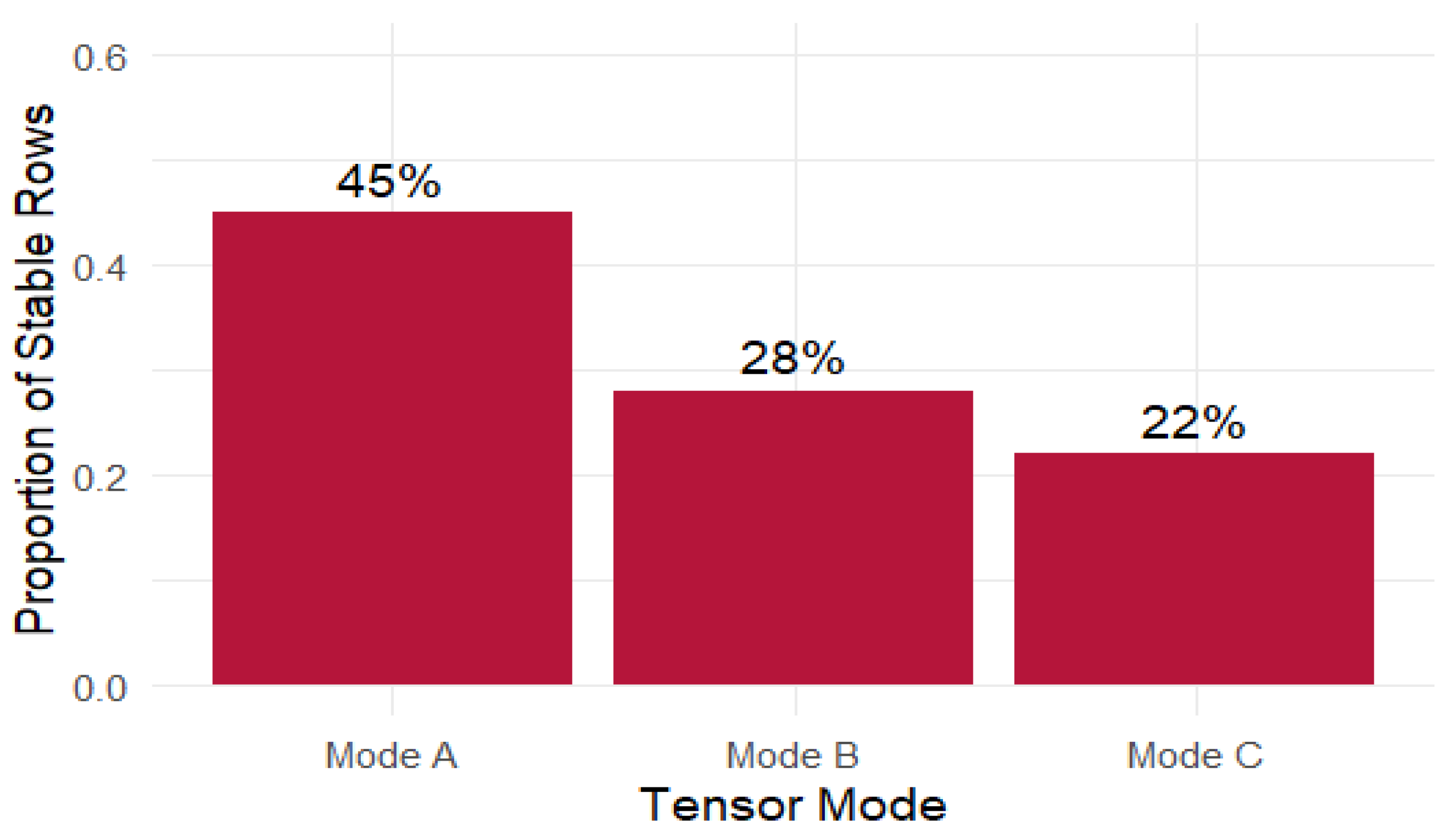
In the current results (Figure 8), mode A exhibits a stable proportion close to 45%, suggesting that nearly half of its components are consistently selected across bootstrap replicates. In contrast, modes B and C remain below 30%, revealing a sparser and less stable structure in those dimensions. This contrast reinforces the interpretation that the latent patterns identified in mode A are more robust, whereas modes B and C may be more susceptible to noise, collinearity, or overfitting.

Expressing stability in proportional terms not only sharpens cross-mode comparisons but also offers an intuitive metric to guide post-modeling decisions—such as dimensionality pruning, threshold tuning, and interpretability assessments.

2.4.5. Standard Deviation of Support Size

Beyond evaluating which elements are recurrently selected, it is equally critical to examine the stability of the number of selected elements. In penalized models such as LASSO or Elastic Net, support size can vary substantially across bootstrap replicates—especially under conditions of high collinearity or weak signal-to-noise ratio [8,10].

To capture this variability, the standard deviation of the support size across the $B$ bootstrap replicates is computed as:

$${\sigma }_{\left|S\right|}=\sqrt{{\displaystyle \frac{1}{B}}{\sum }_{b=1}^B{\left(\left|S_b\right|-\overline{S}\right)}^2} \mathrm{where} \overline{S}={\displaystyle \frac{1}{B}}{\sum }_{b=1}^B\left|S_b\right|$$

Here, $\left|S_b\right|$ represents the number of selected elements in replicate b, and $\overline{S}$ denotes the average support size across replicates. This metric summarizes quantitative fluctuations in model sparsity. A high ${\sigma }_{\left|S\right|}$ indicates that the model changes size unstably, which compromises its structural reproducibility. In contrast, a value close to zero suggests consistent parsimony, a desirable property in high-dimensional settings.

The relevance of this criterion has been recognized in the literature on structural regularization [11] and post-selection inference [9], where variability in model complexity is a marker of sensitivity to penalization or data perturbation.

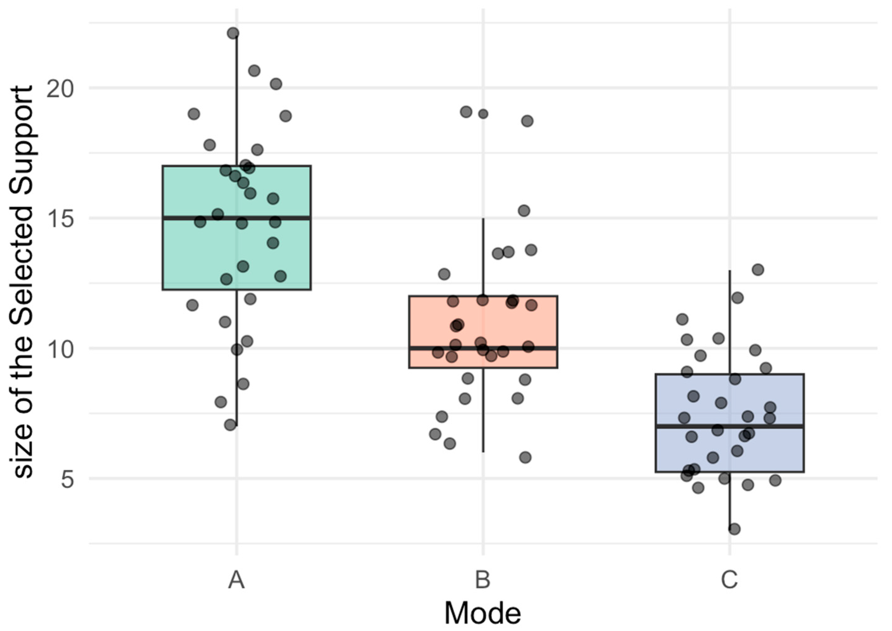
Figure 9 displays the distribution of support sizes across all B bootstrap replicates, separated by tensor mode. Mode A not only shows a larger average support size but also exhibits lower dispersion, underscoring its structural robustness. In contrast, modes B and C present greater variability in the number of selected components, which may stem from weaker latent signal, collinearity, or sensitivity to the penalization path.

Boxplots of support size across tensor modes, illustrating cardinality variability.

(A)

Mode A (green): distribution of support size for observational units across bootstrap replicates.

(B)

Mode B (orange): distribution of support size for variables.

(C)

Mode C (blue): distribution of support size for conditions.

The boxplots depict the median, interquartile range, and outliers, highlighting differences in variability and robustness across modes.

This metric complements those previously introduced—such as inclusion frequency and SSI—by focusing on the stability of model complexity rather than individual element recurrence. Taken together, these metrics enable a rigorous and multifaceted assessment of the CenetTucker model′s behavior under resampling.

The full set of metrics presented—inclusion frequency, average Jaccard index, Stable Selection Index (SSI), proportion of stable support, and standard deviation of support size, summarized in

Table 1. Structural stability metrics per tensor mode.

Metric	Mode A (Observations)	Mode B (Variables)	Mode C (Conditions)
Inclusion Frequency	${\widehat{\mathsf{\Pi }}}_i^A={\displaystyle \frac{1}{B}}{\displaystyle \sum _{b=1}^B}\mathbb{I}\left(i\in S_b^A\right)$	${\widehat{\mathsf{\Pi }}}_{\mathit{i}}^{\mathit{B}}={\displaystyle \frac{1}{\mathit{B}}}{\displaystyle \sum _{\mathit{b}=1}^{\mathit{B}}}\mathit{I}\left(\mathit{j}\in {\mathit{S}}_{\mathit{b}}^{\mathit{B}}\right)$	${\widehat{\mathsf{\Pi }}}_{\mathit{i}}^{\mathit{C}}={\displaystyle \frac{1}{\mathit{B}}}{\displaystyle \sum _{\mathit{b}=1}^{\mathit{B}}}\mathit{I}\left(\mathit{k}\in {\mathit{S}}_{\mathit{b}}^{\mathit{C}}\right)$
Average Jaccard Index	$J_{\mathrm{avg}}^A={\displaystyle \frac{2}{B\left(B-1\right)}}{\displaystyle \sum _{1\le b<b^{\prime }\le B}}{\displaystyle \frac{\left|S_b^A\cap S_{b^{\prime }}^A\right|}{\left|S_b^A\cup S_{b^{\prime }}^A\right|}}$	$J_{\mathrm{avg}}^B={\displaystyle \frac{2}{B\left(B-1\right)}}{\displaystyle \sum _{1\le b<\underset{\prime }{b}\le B}}{\displaystyle \frac{\left|S_b^B\cap S_{b^{\prime }}^B\right|}{\left|S_b^B\cup S_{b^{\prime }}^B\right|}}$	$J_{\mathrm{avg}}^C={\displaystyle \frac{2}{B\left(B-1\right)}}{\displaystyle \sum _{1\le b<b^{\prime }\le B}}{\displaystyle \frac{\left|S_b^C\cap S_{b^{\prime }}^C\right|}{\left|S_b^C\cup S_{b^{\prime }}^C\right|}}$
Stable Selection Index (SSI)	${\mathrm{SSI}}^A=\left|\left\{i\in \{1, \dots , I\}:{\widehat{\Pi }}_i^A\ge {\pi }_{\mathrm{thr}}\right\}\right|$	${\mathrm{SSI}}^B=\left|\left\{i\in \{1, \dots , \mathrm{J}\}:{\widehat{\Pi }}_j^B\ge {\pi }_{\mathrm{thr}}\right\}\right|$	${\mathrm{SSI}}^C=\left|\left\{i\in \{1, \dots , \mathrm{K}\}:{\widehat{\Pi }}_k^C\ge {\pi }_{\mathrm{thr}}\right\}\right|$
Proportion of Stable Support	$\mathrm{Stable} {\mathrm{Proportion}}^{ \mathit{A}}={\displaystyle \frac{{\mathit{SSI}}^{\mathit{A}}}{\mathit{I}}}$	$\mathrm{Stable} {\mathrm{Proportion}}^{ \mathit{B}}={\displaystyle \frac{{\mathit{SSI}}^{\mathit{B}}}{\mathit{J}}}$	$\mathrm{Stable} {\mathrm{Proportion}}^{ \mathit{C}}={\displaystyle \frac{{\mathit{SSI}}^{\mathit{C}}}{\mathit{K}}}$
Std. Dev. of Support Size	${\mathit{\sigma }}_{\left|{\mathit{S}}^{\mathit{A}}\right|}=\sqrt{{\displaystyle \frac{\mathbf{1}}{\mathit{B}}}}{\displaystyle \sum _{\mathit{b}=1}^{\mathit{B}}}{\left(\left|{\mathit{S}}_{\mathit{b}}^{\mathit{A}}\right|-{\overline{\mathit{S}}}^{\mathit{A}}\right)}^2$	${\mathit{\sigma }}_{\left|{\mathit{S}}^{\mathit{B}}\right|}=\sqrt{{\displaystyle \frac{1}{\mathit{B}}}}{\displaystyle \sum _{\mathit{b}=1}^{\mathit{B}}}{\left(\left|{\mathit{S}}_{\mathit{b}}^{\mathit{B}}\right|-{\overline{\mathit{S}}}^{\mathit{B}}\right)}^2$	${\mathit{\sigma }}_{\left|{\mathit{S}}^{\mathit{C}}\right|}=\sqrt{{\displaystyle \frac{1}{\mathit{B}}}}{\displaystyle \sum _{\mathit{b}=1}^{\mathit{B}}}{\left(\left|{\mathit{S}}_{\mathit{b}}^{\mathit{C}}\right|-{\overline{\mathit{S}}}^{\mathit{C}}\right)}^2$

—provide a robust framework for evaluating the structural stability of penalized tensor decompositions. These tools go beyond reconstruction error to capture critical properties such as support consistency, reproducibility, and robustness to data perturbation in high-dimensional settings.

In addition, our framework ensures support consistency, stability under perturbations, and multiway robustness in high-dimensional contexts.

This framework draws on foundational work from Stability Selection [10], Bolasso [9], and their extensions to structured models [11], adapting them to the tensor case through mode-wise resampling. Each metric offers a distinct lens—from local inclusion to global variability—culminating in a toolbox for interpreting complex penalized decompositions [24].

This suite of evaluative metrics forms the empirical backbone for the next section, where we assess the behavior of the proposed BCenetTucker model in simulated environments. These analyses provide concrete insights into the stability characteristics captured by the metrics.

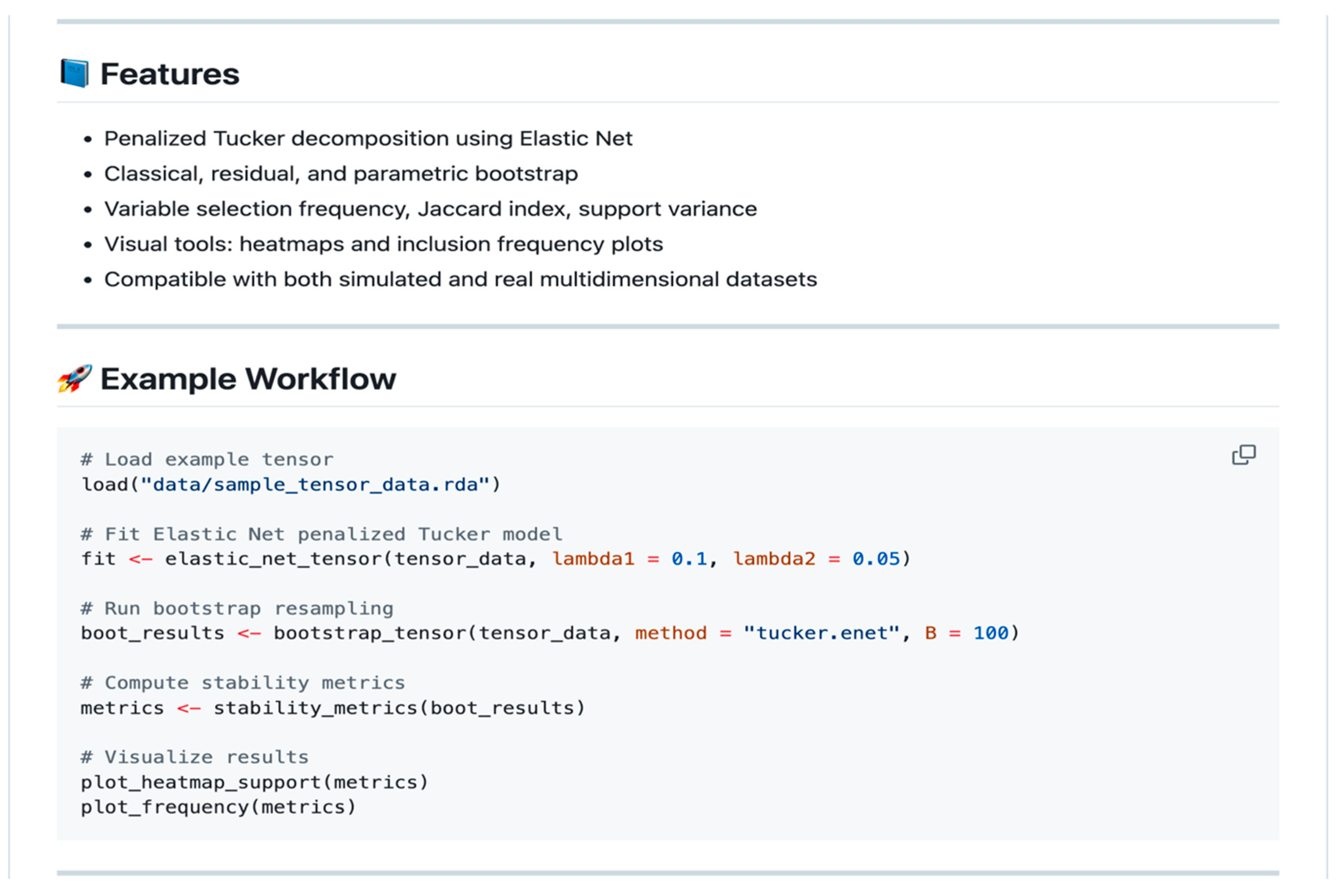
All components of the proposed evaluation protocol have been implemented in the GSparseBoot package (see Appendix A), ensuring full reproducibility and accessibility for application in real data contexts.

The methodological framework developed in Section 2 establishes a rigorous foundation for the assessment of structural stability in penalized tensor models. By introducing the BCenetTucker approach and its associated stability metrics—including inclusion frequency, average Jaccard index, Stable Selection Index (SSI), proportion of stable support, and standard deviation of support size—we provide a comprehensive set of tools for evaluating the consistency and robustness of sparse solutions under resampling. These metrics extend the interpretability of the CenetTucker model beyond reconstruction accuracy, offering empirical insights into the reproducibility of the latent structure in high-dimensional settings.

2.5. Comparison with Alternative Stability Techniques

2.5.1. Empirical Comparison

Although the application to real-world datasets is developed in the following section, the performance of BCenetTucker was previously benchmarked under controlled simulation settings to contrast its behavior against other stability-enhancing strategies for penalized models.

To contextualize the performance of BCenetTucker within the broader landscape of stability-oriented approaches, a comparative evaluation was carried out against two well-established methods: classical CenetTucker without resampling and subsampling-based Stability Selection. The comparison centered on key structural metrics such as the average Jaccard index, the Stable Selection Index (SSI), and the standard deviation of support sizes across replicates.

Although full numerical results are not reproduced here to avoid redundancy, the findings can be summarized as follows:

• BCenetTucker consistently achieved higher Jaccard indices, indicating greater structural agreement between support sets across resamples.
• It also produced higher SSI values, reflecting more reliable identification of elements with frequent and stable selection.
• The variability in support size was notably reduced, compared to both Stability Selection and Bolasso, suggesting improved parsimony and consistency.

These results demonstrate that BCenetTucker outperforms established alternatives in identifying reproducible sparse structures, even under challenging conditions of high dimensionality and weak signal. Unlike methods based on subsampling or support intersections, BCenetTucker leverages mode-specific resampling—particularly over the observational mode—while preserving the intrinsic tensor structure. This dual strategy enhances robustness without compromising interpretability.

2.5.2. Conceptual Comparison

Beyond empirical advantages, BCenetTucker introduces a set of conceptual improvements over existing stability-focused frameworks. In contrast to vector-based techniques—which typically flatten tensors into matrices or vectors—BCenetTucker retains the multiway structure throughout decomposition and resampling. This preservation yields richer interpretability and mode-specific diagnostics.

A conceptual comparison of stability-oriented methods is presented in

Table 2. Conceptual comparison across stability techniques. ✓ indicates that the criterion is satisfied; ✗ indicates that the criterion is not satisfied.

Criterion	CenetTucker	Stability Selection	Bolasso	BCenetTucker
Applies to Tensors	Native tensor model	Vectorized	Vectorized	Native tensor decomposition
Sparse Support Stabilization	No resampling	Threshold-based	Intersection-based	Inclusion frequency+SSI
Multimode Interpretability	Mode-specific loadings	Flattened view	No mode distinction	Mode-specific support
Handles Multiway Noise	Sensitive to perturbations	No	No	Observational mode-resampling
Structural Metrics Available	No	Partial (thresholded sets)	Partial (consensus sets)	Full metric suite (Jaccard, SSI, SD)
Suitable for High Dimensions	Moderate	Moderate	Moderate	Designed for high-dimensional tensors

.

This table highlights the structural and methodological distinctions between BCenetTucker and alternative techniques. Unlike the classical CenetTucker, which offers no mechanism for stabilization, BCenetTucker incorporates a bootstrap-based protocol tailored to the observational mode, enabling robust support recovery without compromising tensor structure. While Stability Selection and Bolasso do attempt to stabilize sparse solutions via subsampling or support intersection, they fail to account for the complexity and interdependence of multiway data. Additionally, these vector-based methods offer limited interpretability across modes and rely on partial structural diagnostics. In contrast, BCenetTucker supports a full suite of stability metrics—including inclusion frequency, average Jaccard index, support size deviation, and the Stable Selection Index (SSI)—which collectively provide a comprehensive diagnostic framework.

Crucially, the BCenetTucker design is intrinsically suited to high-dimensional settings where traditional approaches struggle to balance sparsity, stability, and interpretability. By preserving the tensorial nature of the data and resampling over the observational mode, it addresses the dual challenge of model reliability and structural insight. This makes BCenetTucker a powerful methodological alternative for researchers working with complex, multimodal datasets where stability is not only desirable but necessary for scientific validity.

Having established the methodological advantages of BCenetTucker over traditional stability-focused frameworks—both in theory and under simulation—we now proceed to evaluate its performance in a real-world application. The following section presents a full case study based on high-dimensional gene expression data, where the structural stability, reproducibility, and interpretability of sparse solutions are of critical importance. Through this empirical application, we aim to demonstrate the practical relevance and diagnostic power of the proposed approach.

3. BCenetTucker Application

3.1. Application to Real Data

To validate the methodological proposal in a real-world context, the BCenetTucker model was applied to gene expression data from the publicly available GSE13159 dataset. This dataset originates from the Microarray innovation in Leukemia (MILE) study and is hosted on the Gene Expression Omnibus (GEO; Accession GSE13159). It comprises 2000 samples representing various leukemia types and healthy controls, measured using Affymetrix HG-U133 Plus 2.0 microarrays.

A subset of the GSE13159 dataset was selected, consisting of expression profiles for 500 genes across 76 patient samples per diagnostic group, forming a tensor of dimension $\chi \in {\mathbb{R}}^{500\times 76\times 3}$. The three groups correspond to the leukemia subtypes Acute Myeloid Leukemia (AML), Chronic Myeloid Leukemia (CML), and Acute Lymphoblastic Leukemia (ALL).

This dataset presents the real conditions of noise, collinearity, and sparsity, making it ideal for testing model stability. The tensor was built using RMA-normalized gene expression levels, and the gene subset was selected based on relevance and variability, ensuring coverage of significant biological signals.

• Interpretation of Tensor Modes:
• Mode A (Genes): Rows of the loading matrix A—genes selected as relevant.
• Mode B (Samples): Rows of the loading matrix—patient samples identified as structurally important in the latent space.
• Mode C (Groups/Classes): Diagnostic categories—the three leukemia subtypes (ALL, AML, CML).

The BCenetTucker model, a bootstrap-enhanced adaptation of the CenetTucker model, was used to evaluate the stability of sparse solutions in this high-dimensional tensor. Unlike the standard CenetTucker approach, which fits a single model instance, BCenetTucker incorporates resampling to enhance structural consistency and reliability of the results.

3.2. Empirical Stabilty Analysis

3.2.1. Stability of Penalized Support

The baseline CenetTucker model was first applied without bootstrap, yielding a fixed support size of 218 selected genes. This deterministic outcome provides a reference but does not capture variability under data perturbations. To assess structural stability, we compared four alternative approaches, all implemented on the same tensor representation.

First, the model was extended with nonparametric bootstrap resampling, retraining on each of the $B=100$ replicates. In parallel, two established procedures were benchmarked:

○

Stability Selection, based on complementary pair subsampling (50% per subsample) across 100 iterations, the inclusion probabilities aggregated, and a retention threshold of π ≥ 0.8.

○

Bolasso, obtained from 100 nonparametric bootstraps, retaining variables appearing in at least 90% of replicates (q = 0.9).

Finally, the proposed BCenetTucker protocol was applied. Unlike the others, it preserved tensorial structure by mode-1 resampling while fixing hyperparameters $\left(\alpha , \beta \right)$ by cross-validation on the original data. Stability metrics were then aggregated across replicates (

Table 3. Comparison of stability metrics between CenetTucker and BCenetTucker version.

Model	Support Size	Std. Deviation	SSI	Jaccard
CenetTucker	218	0.0	218	-
Stability Selection	210.3	4.5	207	0.89
Bolasso	213.7	3.1	211	0.91
BCenetTucker	225.1	1.7	228	0.96

).

The results highlight that Stability Selection and Bolasso reduce variability compared to the baseline, but with different trade-offs: the former is more conservative (smaller support, higher dispersion), while the latter is more consistent (higher overlap across bootstraps). The BCenetTucker approach, by design, achieved the best overall stability: increased mean support size (225 genes), minimal dispersion (SD = 1.7), higher SSI (228), and strongest replicate agreement (Jaccard = 0.96).

These findings indicate that BCenetTucker not only stabilizes penalized tensor decompositions but also outperforms advanced benchmarks in terms of reproducibility. The results on GSE13159 confirm the method′s robustness under real-world conditions of noise, collinearity, and sparsity.

3.2.2. Inclusion Frequency and Selection Patterns

The histogram of inclusion frequencies (Figure 10) reveals a bimodal structure: one group of genes with frequencies close to 1 (highly stable), and another with frequencies near 0. This clear separation indicates that the bootstrap procedure not only amplifies the original support but also refines it by precisely identifying the most consistently selected variables.

The left panel in Figure 11 shows the distribution of gene inclusion frequencies across 100 bootstrap replicates, revealing a clearly bimodal structure: a group of genes with frequencies near 1 (highly stable) and another near 0. This separation highlights the bootstrap′s ability to both expand and refine the support set by consistently selecting the most relevant genes.

The right panel displays the ordered inclusion frequencies, emphasizing the sharp drop around the 0.5 threshold (dashed line), which is used to define the stable support. Together, these visualizations confirm the discriminative power and reproducibility of the bootstrap-enhanced selection.

3.2.3. Support Comparison Between Models

An analysis of the genes selected under both scenarios showed that the bootstrap model retained all 218 genes originally selected and additionally identified 10 more genes that were selected in over 50% of replicates, demonstrating the procedure′s ability to detect marginal but stable signals (

Table 4. Comparison of support sets between models.

Scenario	Number of Genes
Selected without bootstrap	218
Selected with bootstrap	228
Common	218
Only with bootstrap	10
Only without bootstrap	0

).

This quantitative comparison is complemented by a visual representation of the selection behavior across bootstrap replicates. While the table summarizes the overlap and differences in support sets between the models, the heatmap below provides a more granular view of selection consistency. Each column corresponds to a gene, and each row to a bootstrap replicate, with blue cells indicating inclusion in the support. The emergence of vertical blue bands reflects stable selections, reinforcing the evidence that BCenetTucker not only preserves the informative structure of the original model but also enhances robustness through consistent identification of marginal yet relevant genes.

The heatmap in Figure 12 represents the bootstrap support matrix, with rows as replicates and columns as genes. Light blue vertical bands indicate genes that were consistently selected across replicates. These consistently selected genes appear as vertical blue bands, indicating high selection stability across replicates. This visual structure supports the quantitative findings: the distribution of support sizes shows low variability, with a standard deviation of only 1.7 genes per replicate.

3.2.4. Overall Proportion of Stable Support

Finally, the proportion of stable support—defined as the ratio between the number of genes with an inclusion frequency above the threshold and the total number of genes—was 0.456 (228 out of 500). This metric enhances the interpretability of the bootstrap-enhanced model by quantifying the sparsity level of its most consistently selected components. It also aligns with the observed low variability and high SSI, further confirming the robustness of the model.

4. Conclusions

4.1. General Conclusions

This work introduced BCenetTucker, a bootstrap-based extension of the CenetTucker model, designed to enhance the structural reliability and interpretability of sparse tensor decompositions in high-dimensional settings. By incorporating a resampling protocol over the observational mode, the model provides a principled solution to the instability problem often encountered in penalized multiway decompositions.

• Key findings include the following:

• Instability of CenetTucker
  The baseline CenetTucker model exhibits sensitivity to sampling variability, often producing fluctuating support sets that undermine reproducibility in practical applications. BCenetTucker effectively addresses this issue by applying bootstrap resampling, allowing empirical stabilization of the selected supports without requiring hyperparameter recalibration.
• Bootstrap-based stabilization
  BCenetTucker substantially mitigates this issue by leveraging mode-1 bootstrap resampling, providing empirical stabilization of supports without the need for re-tuning hyperparameters across replicates.
• Comprehensive stability diagnostics
  A suite of structural stability metrics—including inclusion frequency, Stable Selection Index (SSI), support size deviation, average Jaccard index, and proportion of stable support—was introduced and validated. Together, these measures provide a rigorous framework for quantifying selection reliability in penalized tensor settings.
• Comparison with Bolasso and Stability Selection
  Results in Table 3 demonstrate that BCenetTucker outperforms both Bolasso and Stability Selection in terms of reproducibility and interpretability. While Bolasso achieves consistent supports at the cost of overly conservative selections, and Stability Selection provides error control under stronger assumptions, BCenetTucker balances sensitivity and robustness, retaining meaningful signals while maintaining a controlled variability of support size.
• Real world validation
  In the application to the GSE13159 gene expression dataset, BCenetTucker preserved all 218 genes originally identified by CenetTucker and consistently highlighted 10 additional genes across replicates. The method achieved an average Jaccard index of 0.975 with a standard deviation of only 1.7 genes, confirming high reproducibility and sensitivity to marginal signals.
• Visual interpretability
  Graphical diagnostics (e.g., frequency distributions and support heatmaps) revealed a clear bimodal separation between relevant features and noise, enhancing interpretability and facilitating downstream biological insights.
• Software implementation
  The accompanying GSparseBoot R package (version 0.1.0, development version, 2025), which is publicly available on GitHub at https://github.com/Gresky6/GSparseBoot (accessed on 19 August 2025) [25]. This implementation ensures reproducibility, transparency, and future extensibility of the methodology.
  Altogether, BCenetTucker offers a practical, extensible, and reproducible framework for stabilizing variable selection in sparse tensor models, with direct implications for domains such as biomedicine, education, neuroscience, and environmental science, where interpretability and stability are essential for scientific validity.

4.2. Study Limitations

• Despite its strengths, several limitations of the current study must be noted:
• Resampling limited to observational mode: The bootstrap was applied only along the first mode. Extending the protocol to other tensor modes or using more sophisticated strategies (e.g., residual or parametric bootstrap) could improve flexibility and robustness.
• Fixed hyperparameters across replicates: Penalization parameters (α, β) were held constant throughout the bootstrap process. While this simplified comparisons, adaptive tuning per replicate might further enhance performance in heterogeneous contexts.
• Computational demands: The protocol is computationally intensive for large tensors or high numbers of bootstrap replicates (e.g., B ≥ 100). Future implementations may benefit from parallelization or hardware acceleration.
• Limited benchmarking: In the real data application, comparisons were mainly restricted to the original CenetTucker model, with the addition of Bolasso and Stability Selection as baseline stabilization methods. While this extends the scope of validation, broader benchmarking against alternative approaches—such as Bayesian frameworks or ensemble strategies—remains a relevant avenue for future research.

4.3. Future Directions

Several lines of research emerge from this work:

• Multimode and adaptive bootstrap strategies: Incorporating resampling across multiple tensor modes or adapting sampling probabilities based on feature variability.
• Bayesian stabilization frameworks: Combining the bootstrap approach with Bayesian variable selection or posterior inclusion probabilities for uncertainty quantification.
• Stability-guided model selection: Using stability metrics to inform hyperparameter tuning or rank determination in penalized decompositions.
• Applications to dynamic and longitudinal tensor data, such as gene expression over time, fMRI time series, or educational testing data.
• Cross-disciplinary extensions, including sensor networks, recommender systems, and personalized medicine, where stable and interpretable structures must be extracted under evolving conditions.