1. Introduction
Quantum Phase Estimation (QPE) is a quantum computing algorithm that estimates the phase of an eigenvalue or of multiple eigenvalues of a unitary operator
U. To further understand QPE and the problem addressed in this paper, we will first explore some of the mathematical background of quantum mechanics and the derivation of the QPE algorithm [
1,
2,
3,
4]. Quantum mechanics describes physical particles or groups of particles using states (usually denoted with a “ket”
) in a Hilbert space. For this application of quantum computing, the Hilbert space describes particles or groups of particles with states in a Hilbert space spanned by two basis states,
or
. In this case, the particle or group of particles is called a “qubit”, and a general qubit state is denoted
with complex
complex
and
. When a qubit’s state is measured, the wavefunction collapses into one of the basis states with probability
, where the “bra”
or
, with each bra being an element in the dual space to the space in which the ket
lies.
Changing the state of a qubit within the standard QPE circuit is mathematically represented by acting on the state of the qubit with a unitary operator, which preserves the sum of squares of all vector components. Unitary operators are operators in the Hilbert space such that
, where
is the conjugate-transpose of the operator and
is the identity operator. Measurement of a qubit is a non-unitary operation, though, in this context, it is performed at the end of the circuit and is described probabilistically. While not incorporated in this simulation of QPE circuits, another application of non-unitary operations includes circuit noise analysis associated with open system dynamics [
4]. It is often necessary to work with composite systems representing more than one quantum object. In this case, basis states of the whole system,
, are Kroncker products (a specialization of finite-dimensional tensor products) of the individual basis states, denoted, for example, with
or simply as
or
. Operators on the composite state are also Kronecker products of individual operators, so
. We can re-express the qubit state written as a series of 0’s and 1’s into a decimal number by assigning an order to the qubits, then converting the binary string into a decimal number. Thus, we could take the string of qubits
and create the decimal number
. Most of the paper deals with results written in this decimal form.
The QPE algorithm is used in a number of quantum codes and determines the eigenvalues of a general unitary operator U with corresponding eigenvectors, . The eigenvalues have the form , where is the “phase” of the unitary operator. In this paper, we will deal with a restricted situation where we only have one phase to estimate for each unitary operator.
In order to estimate the phase of some unitary operator, we must begin with a circuit with
qubits split into a first and second register with
and
qubits, respectively. Initially, all qubits in the first register are set to the
state and the qubits in the second register are set to an eigenvector of the unitary operator
, where the subscript 2 denotes the fact that this ket refers to the state of the second register. This leads to an initial state of
. We apply a Hadamard gate
H to each qubit in the first register to yield the state in Equation (2):
Following this operation, we apply a controlled unitary operation
times for the
qubit in the first register. A controlled unitary operation, denoted
, will apply the unitary operation to the second register if the control qubit is
and not apply it if the qubit is
with the result shown in Equation (3). This concludes the operations that involve the second register.
The next step in the derivation is to apply the inverse quantum Fourier transform
. The
is based on the inverse discrete Fourier transform (IDFT), which takes a (normalized) vector of complex numbers, say
, and outputs another vector of complex numbers
, where
. The
takes the quantum state in the numerical basis and transforms it to a superposition of all states in the numerical basis with the coefficient of each basis state in the transformation being the IDFT value. The effect of
is to transform the
qubit state
to the state
shown in Equation (4). The
operator is applied to the first register to obtain the final state of the circuit
before measurement shown in Equation (5):
Measurement in QPE is performed only on the first register. Each of the qubits are measured to produce a string of bits, which is then converted into a decimal number between 0 and
. The probability of measuring a given number
is the probability of measuring the state
in the
equation above, and the probability of such a measurement is the modulus squared of the coefficient of state
. Thus, the probability of
given
, denoted
, is shown in Equation (6):
When
can be represented exactly by a decimal string of
n qubits (say
, then this probability distribution
becomes 1 for the numerical value associated with the string of bits representing
(in this case
with 0 otherwise). However, when this is not possible (like for
),
will have non-zero values for all
x. An example of the final circuit diagram is shown in
Figure 1, which depicts a 3-qubit QPE circuit diagram where the unitary operator is a phase gate corresponding to
θ = 1/3 in the probability distribution. Note that an X gate is applied to the second register (q3) to put the second register into an eigenstate of the phase gate. For validation of this work, a 2-qubit version of this circuit was run on the IBM Perth quantum computer.
The process of doing QPE is akin to sampling from
with
and using the results to estimate the exact value of
. The main difficulty with performing QPE on today’s quantum devices is that present-day devices are plagued by noise in spite of mitigation attempts [
5,
6,
7], which adds an unknown term to the distribution. The process of performing QPE on today’s devices is similar to sampling from another distribution
, where
is a proper probability distribution, but the form and effect of
is not known with certainty. It is possible to recreate some types of noise in simulations of quantum circuits, and one type of noise, depolarizing noise, is added in this paper. Examples of
are found in
Section 2.2.
The datasets were created with 21 levels of depolarizing noise so that the model performance on a variety of noise could be evaluated. The researchers sought to have a single, tunable noise parameter for circuit generation, and depolarizing noise was straightforward to implement. Levels of noise from 0 to 0.2 in steps of 0.01 were chosen to represent the range of noise realistically possible, from ideal at 0 to extremely high at 0.2. It is worth noting that this choice was mostly for practical purposes, since it is computationally expensive to perform these simulations. Someone could, however, produce more data with finer than 0.01 steps in noise and go beyond a noise level of 0.2.
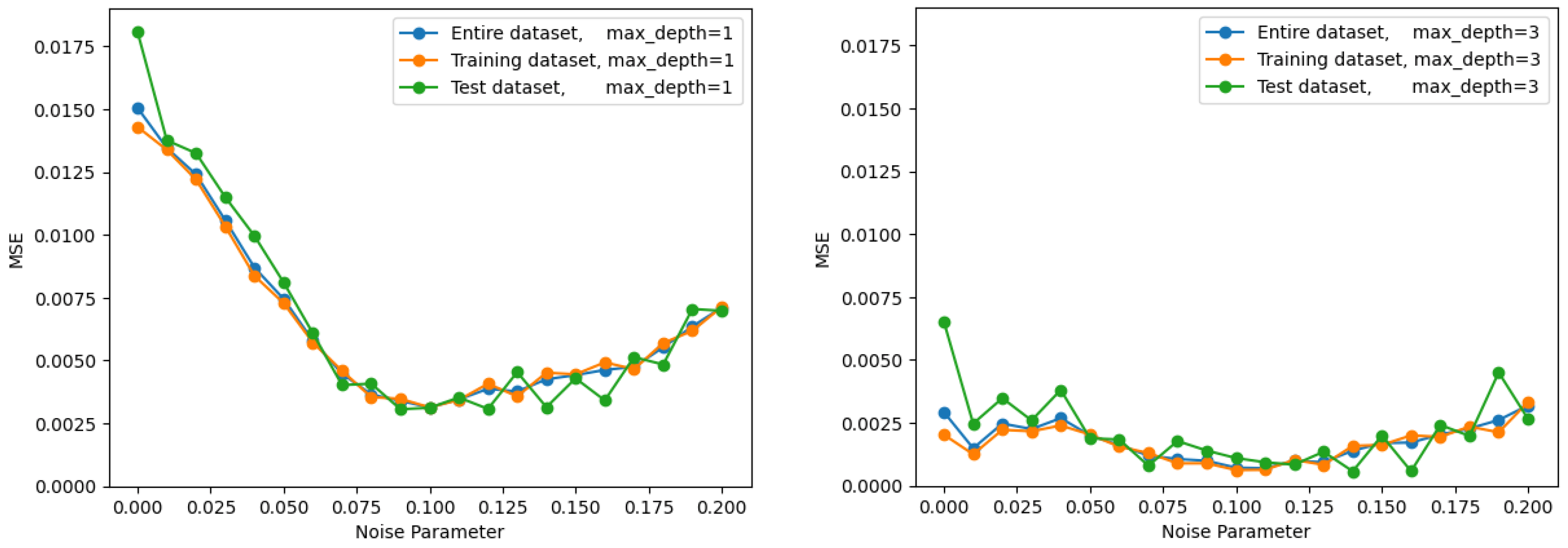
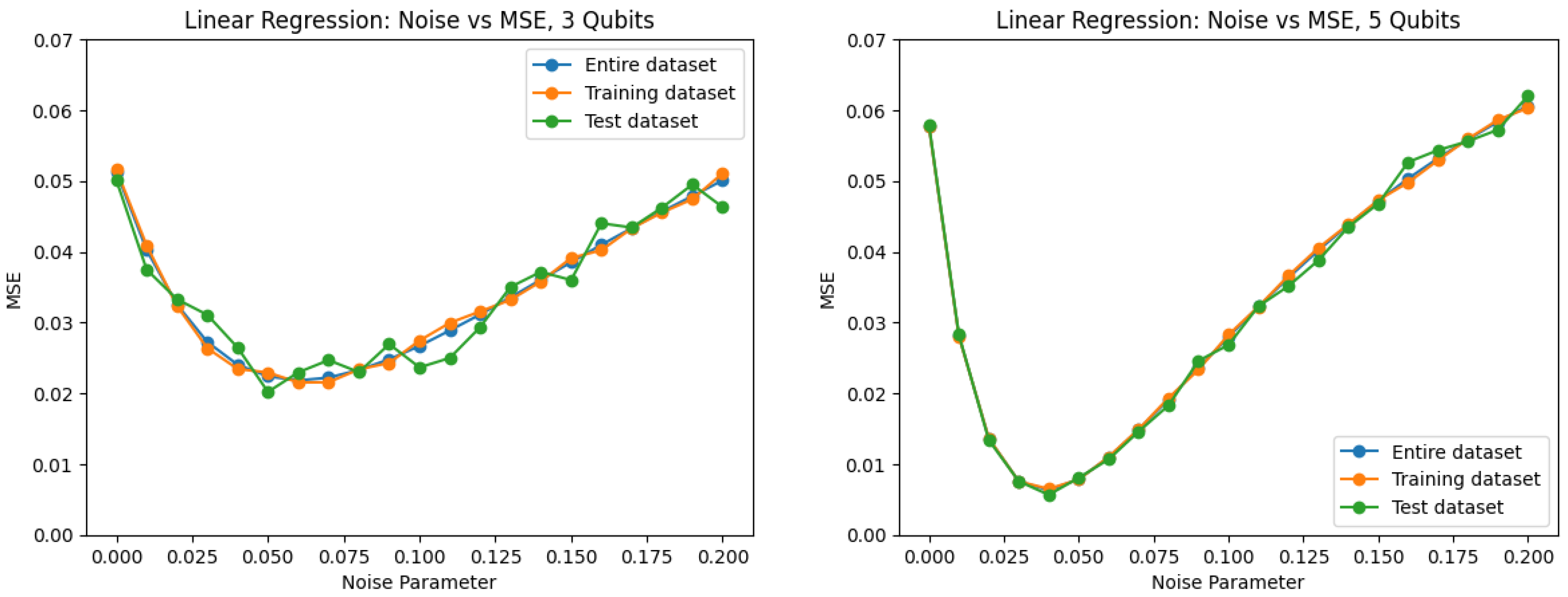
In the training of the models, the level of noise will be uncertain since the quantum phase is estimated by a model, and it is desirable for a model to have consistent predictive performance regardless of the noise level. An example of this is shown in
Figure 2, where the left panel shows a model whose performance varies with noise, and the right panel shows mostly level performance.
1.1. Data Understanding
The phases of data understanding, data preparation, modeling and evaluation from the cross-industry standard process for data mining (CRISP-DM) were followed in this analysis [
8]. The first phase seeks to understand the datasets analyzed in this work. The datasets were generated using a simulated QPE circuit created using IBM’s qiskit, for 2-, 3-, 4- and 5-qubit circuits in a process described in
Section 2.1 and
Section 2.2. In a circuit with
n qubits in the first register, we measure
n qubits once the QPE algorithm described in the introduction is implemented. Each qubit is measured as a 0 or 1. Since there are
n of these qubits, we can measure
possible outputs. When this sequence of
n qubits is considered as a binary number, it can be converted into a decimal number ranging from 0 if all 0’s are measured, to
if all 1’s are measured. A single “shot” of the circuit, corresponding to one sampling from the probability distribution described in the Introduction, is just one of these values in the range 0 to
. The same circuit is run repeatedly to sample many times from the probability distribution. An example for a 2-qubit circuit is presented: if we measure it 400 times and 00 is measured 100 times, 01 is measured 200 times, 10 is measured 50 times, and 11 is measured 50 times, then the feature 00 takes on the value 100/400 = 0.25. In a similar manner, feature 01 takes on the value 200/400 = 0.5, and features 10 and 11 take on the value 50/400 = 0.125. Therefore, the vector of features representing one data point would be [0.25, 0.5, 0.125, 0.125], and we would hope to derive an estimation of the phase from this vector of four features. The process is analogous in systems of higher qubits, and the number of features grows like
. In this experiment, we have generated a dataset with these feature vectors for many different circuits with some associated phase and recorded the noise parameter (described in
Section 2.2) and the phase in order to train the model.
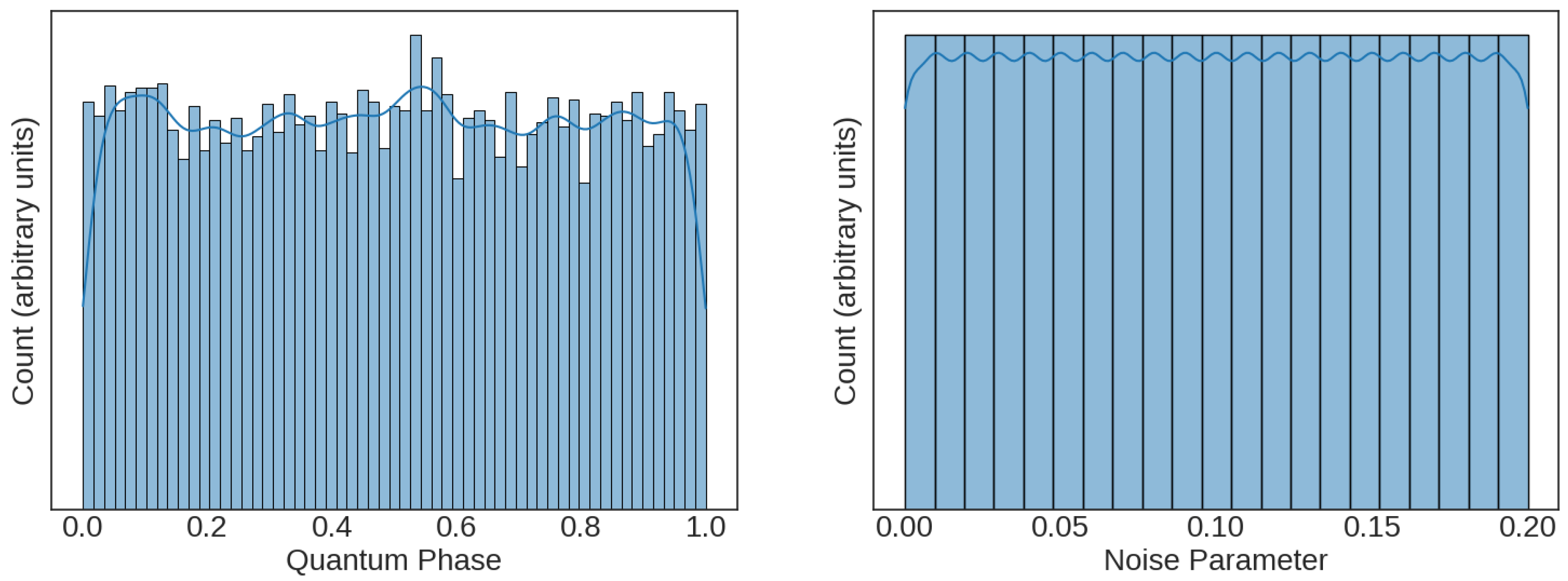
Each row of the dataset contains the transmitted phase, the added noise level and the features that contain the quantum information. For a 2-qubit system there are four features, and the 3/4/5 qubit systems have 8/16/32 features, respectively. For the 2-qubit dataset, histograms with kernel density estimate overlay are presented in
Figure 3 for the transmitted phase (left) and induced noise level (right). Uniform distributions of phase and noise were expected as the transmitted phase was randomly generated, and data were generated uniformly for 21 different noise levels. If these values were unequally distributed, it would be difficult to verify that model performance was consistent across their range. The datasets for the 2-qubit and 5-qubit systems contained 210,000 rows, the 3-qubit dataset contained 52,500 rows, and the 4-qubit dataset contained 105,000 rows.
It is expected that the distributions of each channel in an n-qubit system will be similar, and
Figure 4 confirms this, showing histograms of each channel for the 2- and 3-qubit systems. Verifying this expectation in
Figure 4 increased confidence in the integrity of the large datasets. The non-normal distributions are the expected result of the QPE probability (Equation (6)) and the injected noise levels. In each sub-panel of
Figure 3, the non-normal distributions are explained as follows:
Values near 0 should occur most often, while values close to 1 only occur when the phase exactly lines up with a value of , where is an integer between 0 and .
We expect a small peak at 0.405 since this corresponds to a value of the phase close to , where there are 2 peaks of equal size near 0.405 rather than one largest peak, as is the case when is not close to .
The 4- and 5-qubit system dataset histograms are similar to
Figure 3 and
Figure 4.
1.2. Literature
In the literature, researchers have explored measurement interpretation as an alternative to the highest-peak method [
9] and using machine learning for noise prediction [
10]. The present work is the first instance of machine learning being applied to the problem of interpreting quantum phase estimation measurement output, other than preliminary work performed by the author with a less sophisticated noise model [
11]. The goal of the present work is to find a method for QPE that improves upon the traditional, highest-peak method of estimation.
2. Materials and Methods
The code for the models was prepared and executed within a Python 3.10.12 environment, including sklearn 1.2.2 and keras 2.13.1. Each of the 2/3/4/5-qubit datasets were divided into an 80% training set and a 20% test/holdout set. For neural network algorithms, the training set was further subdivided into 80% training and 20% validation sets. The methods described in this section include the quantum circuit modeling, generation of the dataset, noise generation, details on each of the algorithms and a speed-of-prediction analysis. The methods are summarized in the pseudocode below:
Define the quantum circuit
- ○
Select phase values uniformly between [0, 2π) for generating circuits.
- ○
Create qiskit QPE circuits with qubits = [2,3,4,5] in the first register and 1 qubit in the second register.
- ○
Specify the unitary operator and eigenvector.
Define noise and create datasets
- ○
Introduce depolarizing noise with probability p using qiskit NoiseModel.
- ○
Simulate circuits with 21 noise levels p = [0.00, 0.01, 0.02, …, 0.20].
For dataset in qubits = [2,3,4,5]:
- ○
Create and split datasets with phase, noise level and features for each quantum circuit simulated.
- ○
For algorithm = [linear regression, random forest, XGBoost ensemble, neural network]:
Evaluate overall performance of traditional phase estimation
For noise level p = [0.00, 0.01, 0.02, …, 0.20]
- ○
Evaluate each algorithm to determine performance variation with noise
Training parameters are summarized in Tables 1 and 3
Analyze and compare model performance
- ○
Compare metrics = [MSE, prediction speed, overfitting, variation of accuracy with p] for each algorithm.
- ○
Select the optimal algorithm as the best tradeoff of these metrics.
Validation
- ○
Initialize IBMQ Perth quantum computer using qiskit_ibm_runtime.
- ○
Send circuit output to trained models.
- ○
Compare predictions from models to the analytic results.
2.1. Quantum Circuit Modeling
In order to construct the datasets, a Python package performing high-level quantum computing tasks was used. The package qiskit developed by IBM was used to generate QPE circuits with either 2, 3, 4 or 5 qubits in the first register and 1 qubit in the second register. Aside from the number of qubits in the first register, the distinguishing features of a standard QPE circuit are the specifications of
and
. In our case, regardless of the number of qubits in the first register, the unitary operator whose phase was being estimated was the phase gate
from Equation (6). The phase gate denoted in matrix form, and its eigenvectors
and
are shown in Equations (7)–(9). The corresponding eigenvalues are 1 and
.
The second register is initially in the state
, but an
gate is applied to the qubit transforming it into the
state. Thus, when the unitary operations are applied,
becomes
, so we have
. The values of
estimated by the QPE circuits were chosen uniformly from the interval
, and thus the values of
in each Phase gate were chosen uniformly from the interval
. For each value of
, 21 circuits were generated with different levels of noise, the specifications of which are detailed in
Section 2.2.
2.2. Noise Modeling
Noise was introduced via the qiskit NoiseModel, which contains options for adding many different types of noise to the circuit. In this case, in order to create a tunable parameter of noise, the type of noise added was the depolarizing error of probability
p for both 1 and 2 qubit gates since the circuits in this work have only 1 and 2 qubit gates. The circuit having noise parameter
p essentially means that there is probability
p that, when a 1 or 2 qubit gate is applied, the qubits involved will depolarize, going from their initial state (needed for the algorithm to work) to a mixed state. The further details of quantum circuit noise and depolarizing noise have been explored in the literature; however, they are beyond the scope of this paper [
4,
12,
13].
Figure 5 shows the feature counts when 100,000 shots are simulated within a 4-qubit system with
θ = 1/3. The left/center/right panels show the features with noise levels of
p = 0, 0.05 and 0.2. The result of the absence of noise (left) was a strong, noticeable peak near the best approximation of
θ = 1/3, and a less prominent peak when noise was increased (right) when
p = 0.2.
The result of increasing the noise created a decaying signal in the ultimate distribution. Each time a phase was selected for an n-qubit circuit, a circuit estimating that phase was created in qiskit 21 times, each with a noise parameter p ranging from 0 to 0.2 in steps of 0.01. This resulted in 21 data points for each of the phases that was used to train the models. With the exception of n = 2, the circuits were simulated with shots; essentially, samples from the probability distribution, where is the number of qubits (ranging from 2 to 5). The 2-qubit circuits sampled 10,000 phases, the 3-qubit circuits sampled 2500 phases, the 4-qubit circuits sampled 5000 phases, and the 5-qubit circuits sampled 10,000 phases.
2.3. Metrics and Algorithms
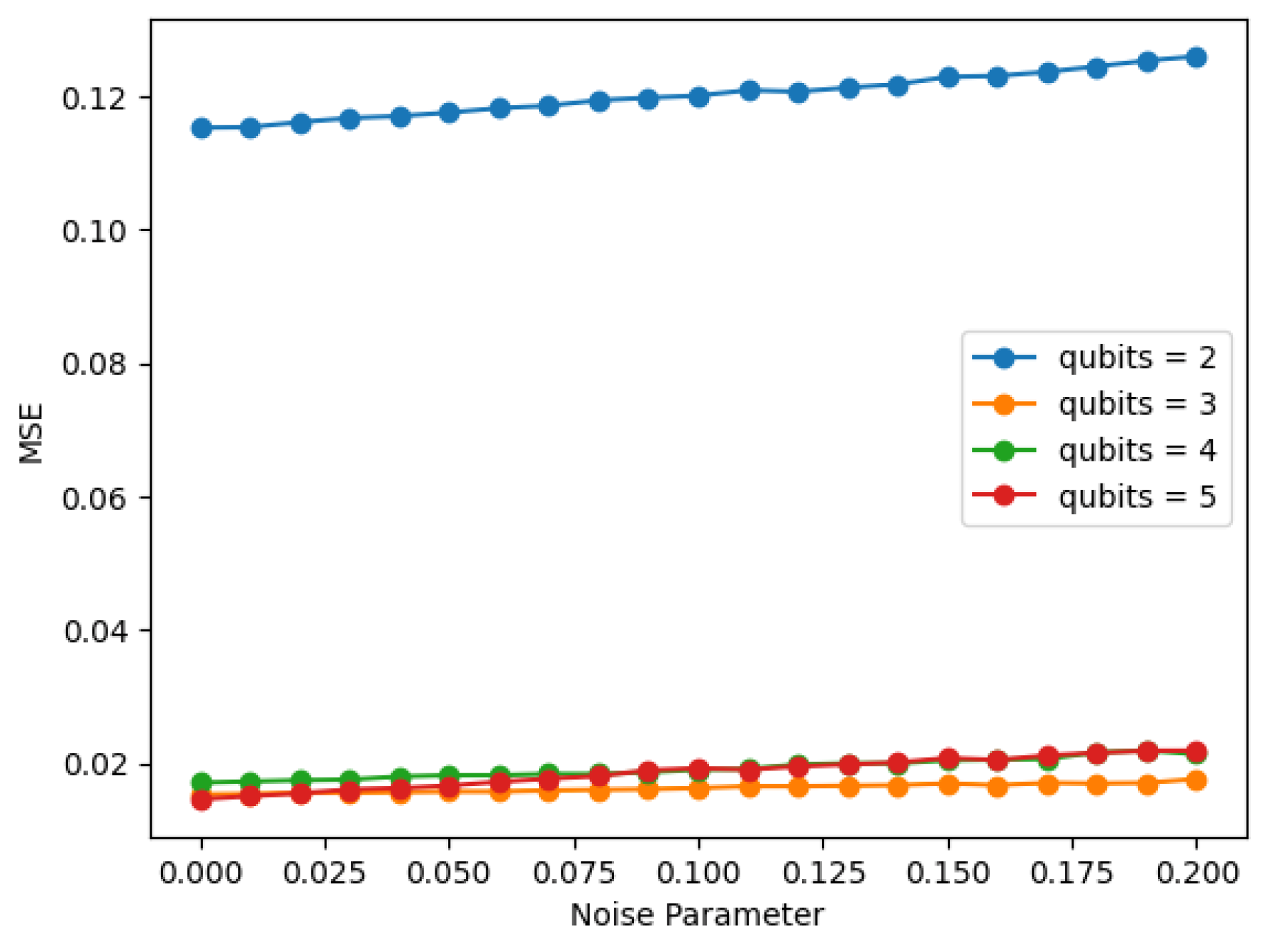
The modeling effort analyzed the potential of five algorithms to predict the quantum phase of a series of qubits: the traditional method of estimating the phase of the eigenvalue of a unitary operator, linear regression, random forest, the ensemble XGBoost algorithm and neural networks. Additionally, the performance of a trivial model was measured by calculating the performance of a model that predicted the mean of the dataset.
The mean squared error (MSE) was selected as the primary performance metric due to its widespread usage in regression problems. Overfitting is another metric used in this work, which is defined as the MSE measured on the training dataset divided by the MSE measured on a holdout/test dataset. A value of overfitting greater than 1 indicates the model does not generalize well on unseen data. A small level of overfitting is tolerated but a high level is undesirable. The performance for all algorithms is summarized in
Section 3.
2.3.1. Traditional Phase Estimation
Recall that the QPE algorithm estimates the phase of the eigenvalue of a unitary operator (i.e., the θ ∈ [0, 1) in the characteristic equation ). The traditional method of estimation only approximates the phase to a precision limited by the number of qubits in the quantum computer. This is performed by taking the most occurring output (in the numerical basis ranging from 0 to , where n is the number of qubits in the first register) and dividing it by . Thus, the traditional estimator for the phase based on a given dataset is the mode of the dataset divided by . This is the traditional method since it can be shown that the mode of the dataset occurs with probability at least and that this is the best approximation of . As an example, if the most common sequence of bits in a 4-qubit first register was 0110, the estimation for would be . This traditional method leaves information about the phase behind in the resulting distribution since values of in the range will all produce distinct distributions, all with mode . That is, given n bits used in the first register, the traditional, mode estimator can only estimate to one part in bits of accuracy. Note that, due to the periodic nature of the complex exponential, near 1 can cause the mode to occur at 0 instead of . For large n, this method can produce a very accurate result, but large numbers of highly accurate qubits are not available on today’s computers. We are seeking to compare how well the traditional method compares to machine learning methods to predict the phase of a unitary operator. Efforts to use machine learning to estimate the phase given the output of the algorithm would be considered successful if they achieved a level of precision greater than that afforded by the traditional and trivial method for the given number of qubits.
The model performance in traditional estimation was calculated on the entire dataset, as opposed to using the test/holdout datasets that the other algorithms used. This is due to the traditional method relying on a calculation based on the features for each row, instead of an algorithm that learns and generalizes on the training data.
2.3.2. Linear Regression
Within Python, the
sklearn ordinary least squares (OLS) linear regression algorithm was applied as it is a common algorithm for regression problems. OLS linear regression is a statistical method used to model the relationship between the predictors (channels) and the dependent variable (quantum phase) by fitting a linear equation to the data. The algorithm minimizes the sum of squared differences between the observed and predicted values of the dependent variable. Other forms of linear regression, such as ridge regression or lasso regression, were not used as the dataset did not suffer from multi-collinearity or have need for feature selection [
15]. Within the
sklearn OLS algorithm, the default Moore–Penrose pseudo-inverse solver was used, and all features were used without interaction terms.
2.3.3. Tree-Based Methods
Two tree-based methods were evaluated in this work: the
sklearn RandomForestRegressor algorithm was evaluated as it performed well in a quantum phase transition problem [
16], and the extreme gradient boosting algorithm XGBoost was selected to investigate the performance of an ensemble algorithm, which can often rival the performance of neural networks. Tree-based algorithms are known to overfit if the maximum depth hyperparameter is too high [
17,
18], and the example in
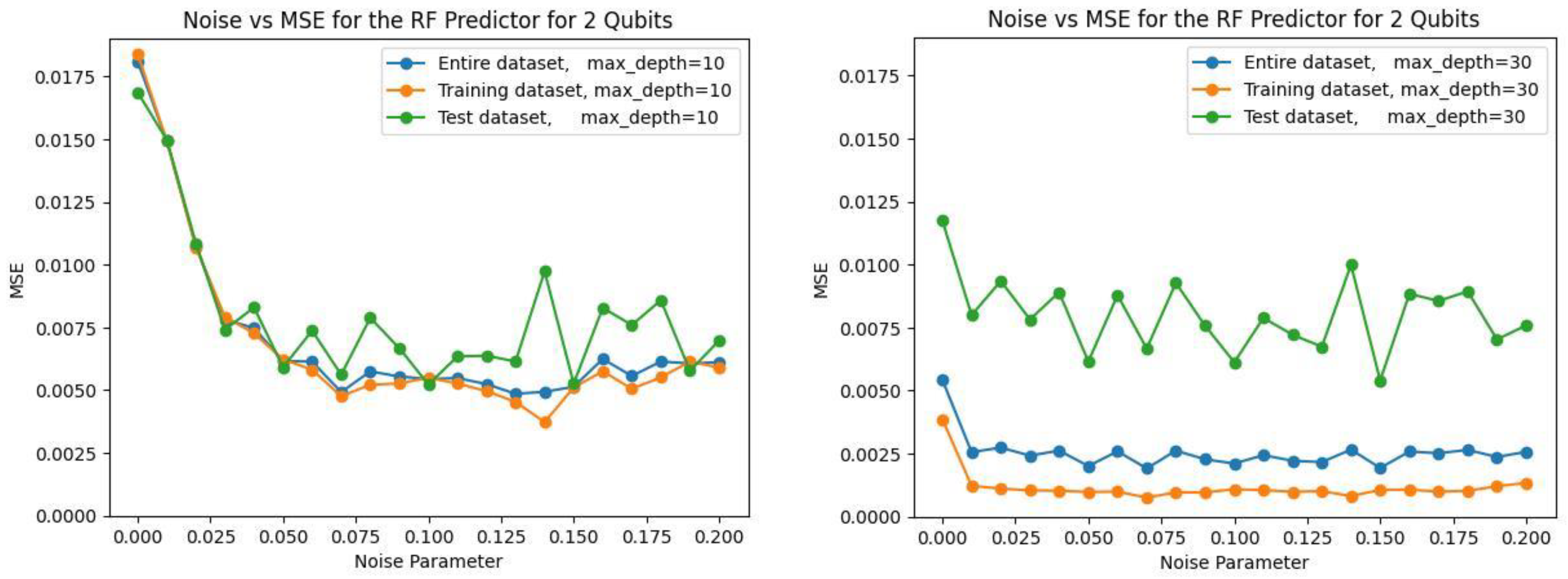
Figure 6 highlights this issue. The right side of the figure shows the training and test dataset performance for max_depth = 30, which overfits the training dataset by 85%. The inferior performance of the green test dataset curve shows that the model has memorized the training data and does not perform well on the test data. The left side of the figure shows the same chart for max_depth = 10, where overfitting is limited to 15%. Even though the “entire dataset” metric makes it seem the max_depth = 30 model is better, it is noteworthy that the mean “test dataset” performance is very similar to the overfit max_depth = 30 model. The max_depth = 10 model will generalize better on unseen data, and its performance is equivalent on unseen data.
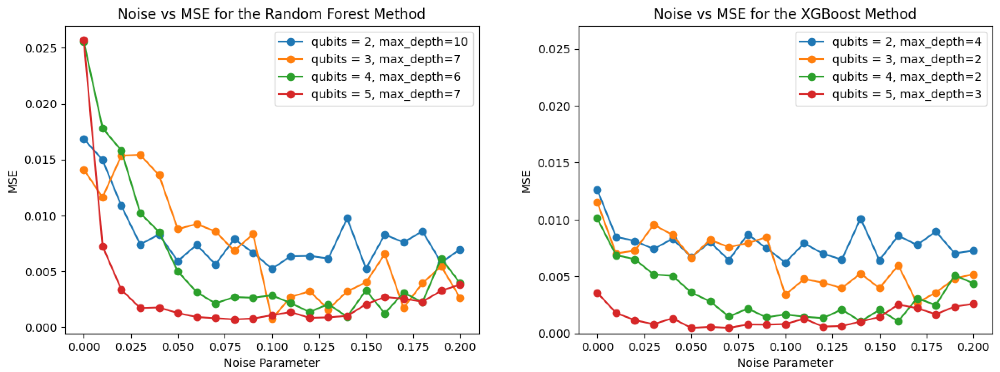
The random forest algorithm used 200 trees, a squared error criterion, and the maximum depth parameter was swept to determine the best performance that can be obtained with <15% overfitting. In this analysis, the maximum depth was varied from 1 to 11 for each of the 2/3/4/5-qubit models to determine this parameter.
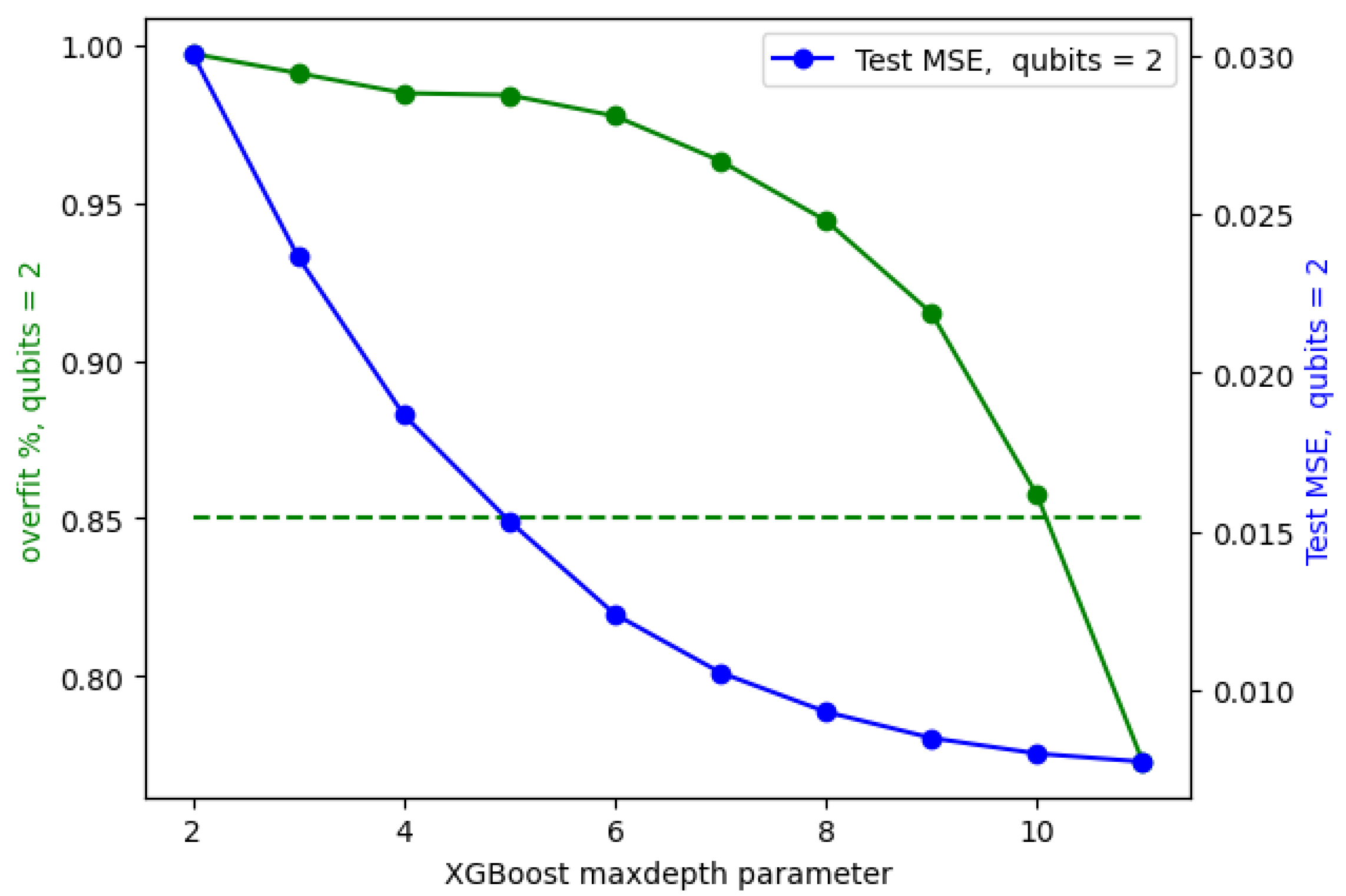
Figure 7 shows the evaluation process for the 2-qubit model, where a model was created for each value of maximum depth ranging from 1–11. In
Figure 7, the
x-axis is the maximum depth parameter, and the blue line shows that model MSE improves with a higher depth parameter. The green line plots overfitting (defined in
Section 2.3), showing that the algorithm quickly overfits as the maximum depth parameter is increased. The dashed green line shows a 15% overfitting threshold, which, in this case, is exceeded for a value of maximum depth > 10. The maximum depth parameter where overfitting is limited to <15% is provided in
Table 1 for the 2/3/4/5-qubit models, for both the random forest and XGBoost algorithms.
Similar to the random forest algorithm, the XGBoost maximum depth parameter was swept to determine the highest depth parameter that can be used with <15% overfitting. The results of the sweep are presented in
Table 1 for the 2/3/4/5-qubit models, and it can be seen that the XGBoost algorithm overfit the data at lower values of maximum depth.
2.3.4. Neural Network
The Python keras framework was used to create neural network models using a sequential architecture, with a baseline model and hyperparameter-tuned model created for each dataset. The baseline model consisted of four layers: a TensorFlow preprocessing normalization layer to standardize the inputs, two hidden dense layers of ReLU neurons with L2 = 0.001 regularization, and an output dense layer consisting of a single linear neuron signifying a regression problem. An adaptive moment estimation (Adam) optimizer was selected as the optimizer, and the model was trained for 240 epochs at an initial learning rate of 0.2. To aid in training, a callback halved the learning rate every 30 epochs. A 5–100 neurons sweep was conducted to establish a starting point for the multi-dimensional hyperparameter optimization.
The baseline neural network size was informed by Widrow’s rule of thumb, which relates the number of neurons to the number of data points
P, the number of weights (neurons × (inputs + 1)), and the desired error level according to Equation (10) [
19].
The maximum recommended neuron count for the 2/3/4/5-qubit models was then calculated as 1250/175/185/190 neurons (respectively) by solving Equation (10) for neurons. The inputs to the equation were the average 3% error level in this work, 4/8/16/32 inputs, and the 210,000/52,500/105,000/210,000 row dataset size. The 2-qubit recommendation was much larger than the others due to possessing only four inputs and having 210,000 rows of data. Maximum neuron counts in the hyperparameter sweeps were limited to within 3x of the Widrow recommendations.
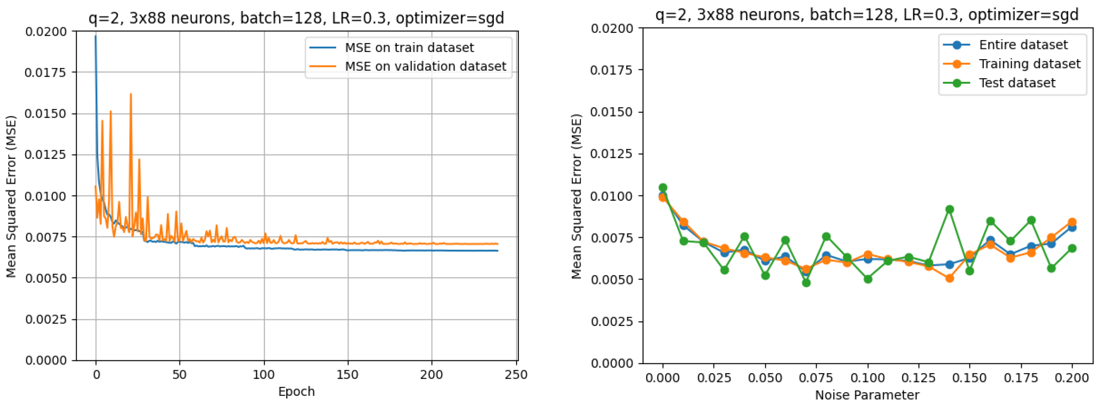
Within Python, the neural network model’s hyperparameters were tuned using the Adaptive Experimentation Platform (Ax) library. Ax uses Bayesian optimization for numeric hyperparameters, which include the initial learning rate, number of hidden layers, neurons per layer and batch size. Bandit optimization was used to tune the categorical optimizer hyperparameter. The training dataset was split into training and validation, and the hyperparameters were tuned using the validation dataset. After tuning to find the optimal set of hyperparameters, the final metrics were calculated using the test/holdout dataset. The optimal hyperparameters are presented in
Section 3.5 for each model.
2.4. Speed Analysis and Validation on an IBM Device
If a research application were to require a fast prediction time, the time to execute
model.predict() on each dataset was recorded within Python for each algorithm in order to provide this for a researcher’s consideration. A 2-qubit datapoint was obtained from an IBMQ quantum computer by running
qiskit_ibm_runtime [
20]. The quantum computer was
IBMQ_perth, whose qubit layout is shown in
Figure 8. This quantum computer is no longer available for use but the following specifications have been reported for this device in the literature [
21,
22] and information about the job is retrievable [
23]. It is a 7 superconducting transmon qubit quantum computer with a quantum volume of 32. The basis gates are the CNOT, I, RX, SX, and X gates. The T1 time = 168.85 msec and the T2 time = 132.51 msec. The median CNOT error rate = 8.690 × 10
−3 and the median SX error rate = 2.8060 × 10
−4. The median readout error = 2.930 × 10
−2.
There was no use of any error mitigation from qiskit_ibm_runtime for these data. The phase and channels were 1/3 and [0.092, 0.58175, 0.181, 0.14525], respectively. This data point used for validation was directly extracted from the IBM Quantum jobs page on the date of the experiment. The best 2-qubit model was then used to predict this datapoint, and the prediction was compared to the actual phase and the traditional method of phase estimation.
4. Discussion
An ideal QPE post-processing algorithm would predict the phase accurately in the presence of noise, have non-varying performance across a variety of noise levels, possess minimal overfitting, and have a rapid prediction time so that lag is not induced into any quantum computing applications where QPE is an intermediate step. No algorithm was a clear winner when considering these four criteria, as the lowest-error model (Ax-tuned NN) was also the slowest predictor; the algorithm with the lowest overfitting (linear regression) and fastest prediction time had the highest error level and a high degree of variation of error with noise. The XGBoost ensemble method was judged to be the best tradeoff between these criteria, as it had the second-best error level, second-best prediction time and low variation of error with noise. It is worth noting that this is not necessarily a negative result, as not all applications require speed or maximum accuracy.
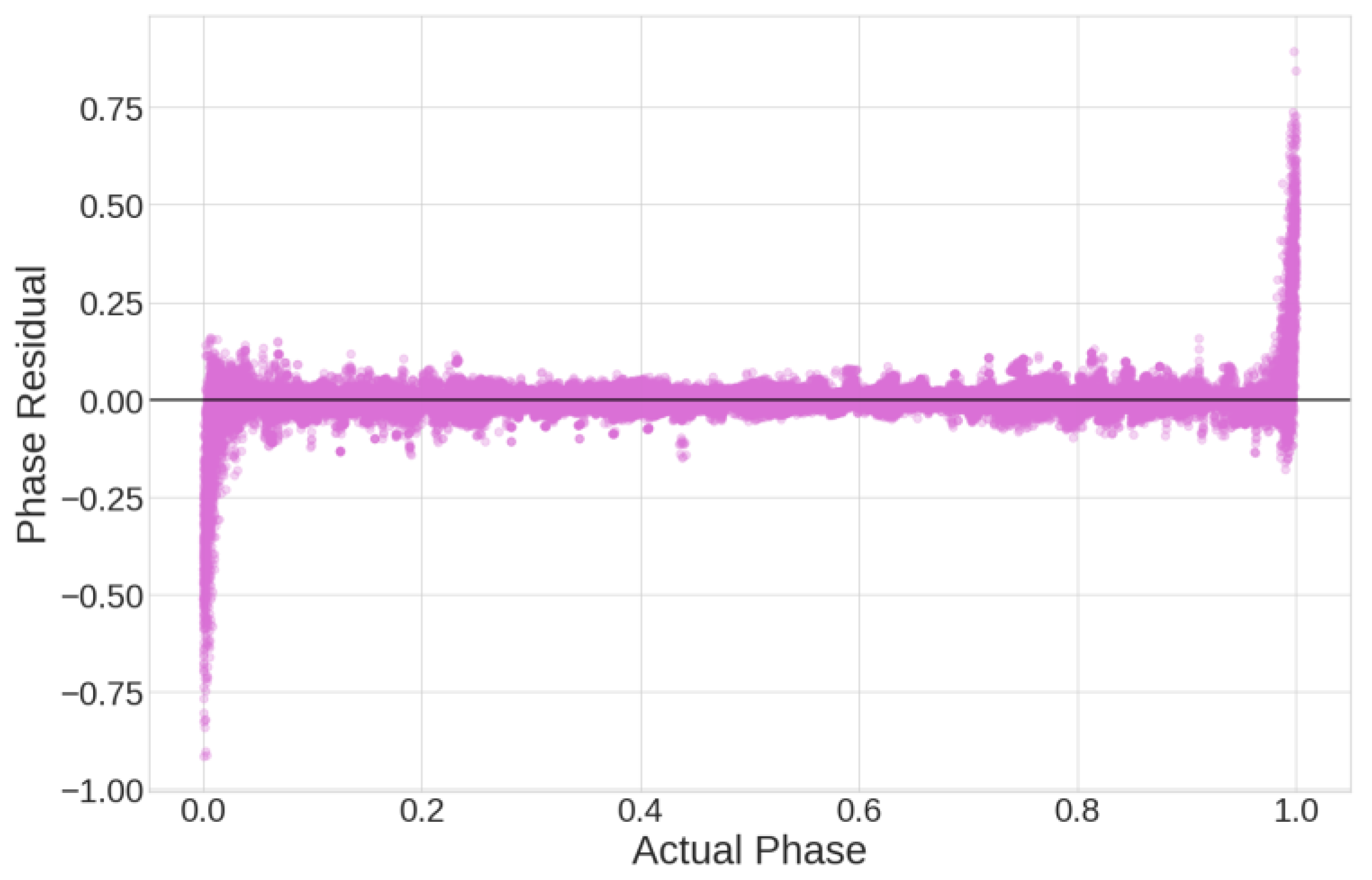
A residual analysis for the 5-qubit XGBoost algorithm is shown in
Figure 13, and it can be seen that the model struggles to predict the boundary phases near 0 and near 1 since the phase is an angular measurement that passes continuously between 0 and 1.
The second-best algorithm was the Ax-tuned NN models as they had the lowest error level and variation of error with noise. Of the three optimizers compared, the stochastic gradient descent (SGD) optimizer was best for all datasets. Other generalizations noted across all datasets were that the best performance was achieved with high initial learning rates, three or four hidden layers, and batch sizes (128–522) that were low in comparison to the 52,500–210,000 row dataset size.
Limitations and Drawbacks
There are a few limitations of this method of enhancing QPE that are important to consider. First, this method requires the simulation of large datasets, which is computationally expensive for small qubit systems (like those considered here) and nearly impossible for many qubit systems since the computational difficulty is exponential. Since the accuracy of the traditional method increases exponentially with the number of qubits as well, a QPE system of several qubits free of noise would be better than the best performance of our method. Therefore, the useful application for this type of improvement to the standard QPE approach lies in circumstances where only a few qubits are available in the first register. This is, however, the circumstance in which the field of quantum computing finds itself now.
More specific limitations in this experiment include the fact that only one type of error was examined in the simulated circuits. For a more complete picture, Pauli measurement, depolarizing, thermal relaxation, and reset errors (among many others) would need to be inserted into the simulations, though this would require more simulation for every type of noise that is modeled. Furthermore, only one phase was present in the distributions. For general applications, the state of the second register may not be an eigenstate of the unitary operator, which leads to multiple phases affecting the probability distribution from which we sample. Our models are not applicable to these scenarios. Simulations of more general situations with multiple types of error and multiple phases are underway in order to train more advanced machine learning models. Finally, this experiment only measured performance with absolute error in phase, not the periodic error for the phase, , given by . It is possible to train models and perform analysis with this periodic error, and having both sets of models may be desired by some researchers. This is, again, an opportunity for further work.
5. Conclusions
In this work, QPE using machine learning was shown to offer significant potential to improve phase estimation in the presence of depolarizing noise. In this work, simulated quantum datasets were generated for 2/3/4/5-qubit systems, and each row of each dataset contained the quantum register, the phase to be predicted, and 21 different levels of depolarizing noise that were added to the phase. The phase was transformed to range from 0–1, and the noise level ranged from 0–0.2. The mean squared error was used as the primary model performance metric, and a 6x–36x improvement in model performance was noted, depending on the dataset, when comparing the Ax-tuned neural network to the highest-peak estimator.
The model prediction speed, overfitting level and variation in accuracy with noise level was determined for five machine learning algorithms. The prediction speed ranged from 10,000–51,800,000 records per second, which could constrain the applications of the slowest algorithms. Overfitting ranged from 1–15%, and the MSE for the neural networks ranged from 0.0069–0.0005. While the XGBoost ensemble algorithm did not possess the lowest error level, it was judged to be the best tradeoff between the four criteria due to its error level, prediction time and low variation of error with noise. The lowest-error model (neural network) was also the slowest predictor; the algorithm with the lowest overfitting and fastest prediction time (linear regression) had the highest error level and a high degree of variation of error with noise. A machine learning prediction was made on a 2-qubit datapoint obtained from an IBMQ 2-qubit quantum computer, and it demonstrated a significant improvement over the traditional method. The models and experiment possess the potential to increase the QPE accuracy for emerging quantum computers.

