Article

Motion Correction for Brain MRI Using Deep Learning and a Novel Hybrid Loss Function

1
Department of Diagnostic Radiology and Nuclear Medicine, University of Maryland School of Medicine, 670 W. Baltimore Street, HSF-III, Baltimore, MD 21201, USA
2
Department of Mathematics and Center for Scientific Computation and Mathematical Modeling, University of Maryland, College Park, MD 20742, USA
*
Author to whom correspondence should be addressed.
Algorithms 2024, 17(5), 215; https://doi.org/10.3390/a17050215
Submission received: 18 March 2024 / Revised: 2 May 2024 / Accepted: 7 May 2024 / Published: 15 May 2024

Abstract

:
Purpose: Motion-induced magnetic resonance imaging (MRI) artifacts can deteriorate image quality and reduce diagnostic accuracy, but motion by human subjects is inevitable and can even be caused by involuntary physiological movements. Deep-learning-based motion correction methods might provide a solution. However, most studies have been based on directly applying existing models, and the trained models are rarely accessible. Therefore, we aim to develop and evaluate a deep-learning-based method (Motion Correction-Net, or MC-Net) for suppressing motion artifacts in brain MRI scans. Methods: A total of 57 subjects, providing 20,889 slices in four datasets, were used. Furthermore, 3T 3D sagittal magnetization-prepared rapid gradient-echo (MP-RAGE) and 2D axial fluid-attenuated inversion-recovery (FLAIR) sequences were acquired. The MC-Net was derived from a UNet combined with a two-stage multi-loss function. T1-weighted axial brain images contaminated with synthetic motions were used to train the network to remove motion artifacts. Evaluation used simulated T1- and T2-weighted axial, coronal, and sagittal images unseen during training, as well as T1-weighted images with motion artifacts from real scans. The performance indices included the peak-signal-to-noise ratio (PSNR), the structural similarity index measure (SSIM), and visual reading scores from three blinded clinical readers. A one-sided Wilcoxon signed-rank test was used to compare reader scores, with p < 0.05 considered significant. Intraclass correlation coefficients (ICCs) were calculated for inter-rater evaluations. Results: The MC-Net outperformed other methods in terms of PSNR and SSIM for the T1 axial test set. The MC-Net significantly improved the quality of all T1-weighted images for all directions (i.e., the mean SSIM of axial, sagittal, and coronal slices improved from 0.77, 0.64, and 0.71 to 0.92, 0.75, and 0.84; the mean PSNR improved from 26.35, 24.03, and 24.55 to 29.72, 24.40, and 25.37, respectively) and for simulated as well as real motion artifacts, both using quantitative measures and visual scores. However, MC-Net performed poorly for images with untrained T2-weighted contrast because the T2 contrast was unseen during training and is different from T1 contrast. Conclusion: The proposed two-stage multi-loss MC-Net can effectively suppress motion artifacts in brain MRI without compromising image quality. Given the efficiency of MC-Net (with a single-image processing time of ~40 ms), it can potentially be used in clinical settings.

1. Introduction

Magnetic resonance imaging (MRI) is a widely used medical imaging modality for visualizing and quantifying the anatomy and function of tissues and organs as well as pathologic processes [1]. MRI provides high spatial resolution and many different tissue contrasts, making it superior to many other imaging modalities for detecting and characterizing soft tissue (e.g., brain, abdominal organs, and blood vessels) and pathologies.
Because it involves the sequential spatial encoding of an imaging object, MRI is relatively slow and can take several minutes for a typical 3D volume scan. This prolonged image acquisition process makes MRI sensitive to motion [1,2]. Unfortunately, motion by human subjects is unavoidable and can be caused even by involuntary physiological movements, such as respiration and cardiac motion, and unintended patient movements. Motion-induced image artifacts can drastically deteriorate image quality and reduce diagnostic accuracy [2]. For example, Andre et al. reported that almost 60% of 192 clinical brain MRI scans analyzed were contaminated with motion artifacts [3]. Among these, 28% were marginally diagnostic to non-diagnostic and needed to be repeated. Because of motion-induced image artifacts, the annual loss in revenue per MR scanner can be over USD 100,000 for brain studies alone [3].
A range of prospective correction strategies have been developed to attenuate motion artifacts [4,5,6,7,8], but they commonly have limitations such as low scanner platform accessibility, applicability to specific MRI sequences only, and limitations in correcting different types of motion artifacts (e.g., in-plane versus through-plane movements). Therefore, retrospective motion correction by means of post-processing provides a good complement. One promising approach involves deep learning (DL) [1,2,9,10,11], using deep convolutional neural networks (DCNN) or other network architectures with supervised learning. Given sufficient training pairs (inputs and reference images), DCNNs can be trained to recognize the transformation from the input (motion-corrupted image) to the reference (motion-free image). Trained DCNNs have successfully been used to solve many challenging and clinically important problems, e.g., arterial spin-labeling perfusion MRI denoising [12,13], image segmentation [14,15], and image registration [16,17].
DCNNs appear to be well-suited for retrospective correction of motion artifacts since there are no obvious conventional algorithms for solving this problem, and yet expert readers can “read through” the artifacts to some degree. Recent studies demonstrate that DCNNs can be used to attenuate motion artifacts in brain MRI scans using a data-driven approach without prior knowledge.
The purpose of this study was to implement and evaluate a deep neural network architecture and loss function for motion correction. The methodology and scope of this study are different from those of previous studies. We summarize our contributions as follows.
  • First, a new loss function was developed, which contains an L1 component for penalizing overall image artifacts and a total variation (TV) component to penalize the loss of image details such as boundaries. Accordingly, a two-stage training strategy was implemented to first minimize the overall motion artifacts and then consider both the residual motion-induced artifacts and the loss of image details such as boundaries.
  • Second, the generalizability of the trained model was assessed using images with orientations and contrast different from those of the training data.
  • Third, to ensure rigor and demonstrate clinical utility, in-depth evaluations were made using different levels of synthetic motions and in vivo data from patients, using both objective performance indices and subjective reading conducted by experienced clinicians. Motion-free images were also used to assess potential over-corrections made by the trained DL networks.
  • Finally, to allow other researchers to reproduce our work or use the presented methods to process their own data, we have provided the code and sample data at https://github.com/MRIMoCo/DL_Motion_Correction (accessed on 10 October 2023).
This paper is organized as follows. In the Related Works Section, we review previous work related to our study. We introduce the proposed MC-Net, the data sets used to train and evaluate the MC-Net, and the evaluation methods in the Materials and Methods Section. We provide experimental results in the Results Section. In the Discussion Section, we discuss our findings and the limitations of our study. Finally, we conclude our paper in the Conclusions Section.

2. Related Works

With the recent development of deep learning approaches, especially DCNN, several DCNN-based methods have been proposed to solve the motion correction problem in a data-driven manner. For instance, variation auto encoders (VAEs) and generative adversarial networks (GANs) have been employed for the retrospective correction of rigid and non-rigid motion artifacts in motion-affected MR scans [1]. GANs have also been used for motion correction in multi-shot MRI [9]. A conditional GAN improved the image quality of predicted motion-corrected images to a greater extent than motion-corrupted images [18]. In [19], a retrospective motion correction method that combined the advantages of classical model-driven and data-consistency-preserving methods for fast and robust motion correction was proposed and evaluated. In a recent study, a DCNN was also used for estimating the severity of motion artifacts in under-sampled MRI data, providing useful information for use in the reconstruction method [20]. Finally, an encoder–decoder network was able to suppress motion artifacts with motion simulation augmentation [2]. A comprehensive survey of deep learning for motion correction has been provided in [21]. Although great progress has been made by applying DCNNs to the motion correction problem, there is still much room for improvement. To the best of our knowledge, the source codes of most studies [1,9,18,19,20] are not publicly available, making it difficult for researchers to build and improve upon prior studies. Also, many previous approaches directly utilized existing DCNN models for motion correction. Hence, we aimed to develop a customized DCNN model for motion correction using publicly available source code.

3. Materials and Methods

3.1. MC-Net

The proposed deep-learning-based method (Motion Correction Net, i.e., MC-Net) takes a motion-corrupted image as input and outputs a motion-corrected image. This method has a modified UNet [22] (Figure 1) as its neural network structure. The MC-Net was trained with a two-stage training strategy using a hybrid loss function, L, that combines L1-loss and TV-loss [23]. By integrating TV-loss, the hybrid loss function encourages the model to produce output images with low total variation that can have sharp edges and reduced motion artifacts. The outer exponent is 1.25, as suggested in [22]:
L = a l p h a L 1 + b e t a T V
L 1 = i , j I i , j I 0 i , j
T V = i , j I i + 1 , j I i , j 2 + I i , j + 1 I i , j 2 1.25
where I and I0 are a corrupted image and a motion-free image, and i and j are row/column indices. During the first training stage, we used L1-loss only [(alpha, beta) = (1, 0)] to suppress overall motion-induced artifacts. The pre-trained stage 1 model was then fine-tuned in stage 2 by turning on the TV-loss component [(alpha, beta) = (1, 1)]; this penalizes the total variation in relation to boundary artifacts in addition to the overall artifacts.

3.2. Motion-Corrupted Images

Images with simulated motion artifacts were based on deidentified brain MRI scans from 52 human subjects (50 males and 2 females, 48.6 ± 9.1 years old) previously enrolled in research studies. All data were acquired using a 3T scanner (TIM Trio, Siemens Healthcare, Erlangen, Germany). The ability of MC-Net to correct real (non-simulated) images with motion artifacts was assessed using motion-corrupted scans from five additional healthy subjects (2 males and 3 females, age 19 ± 4.9 years old).
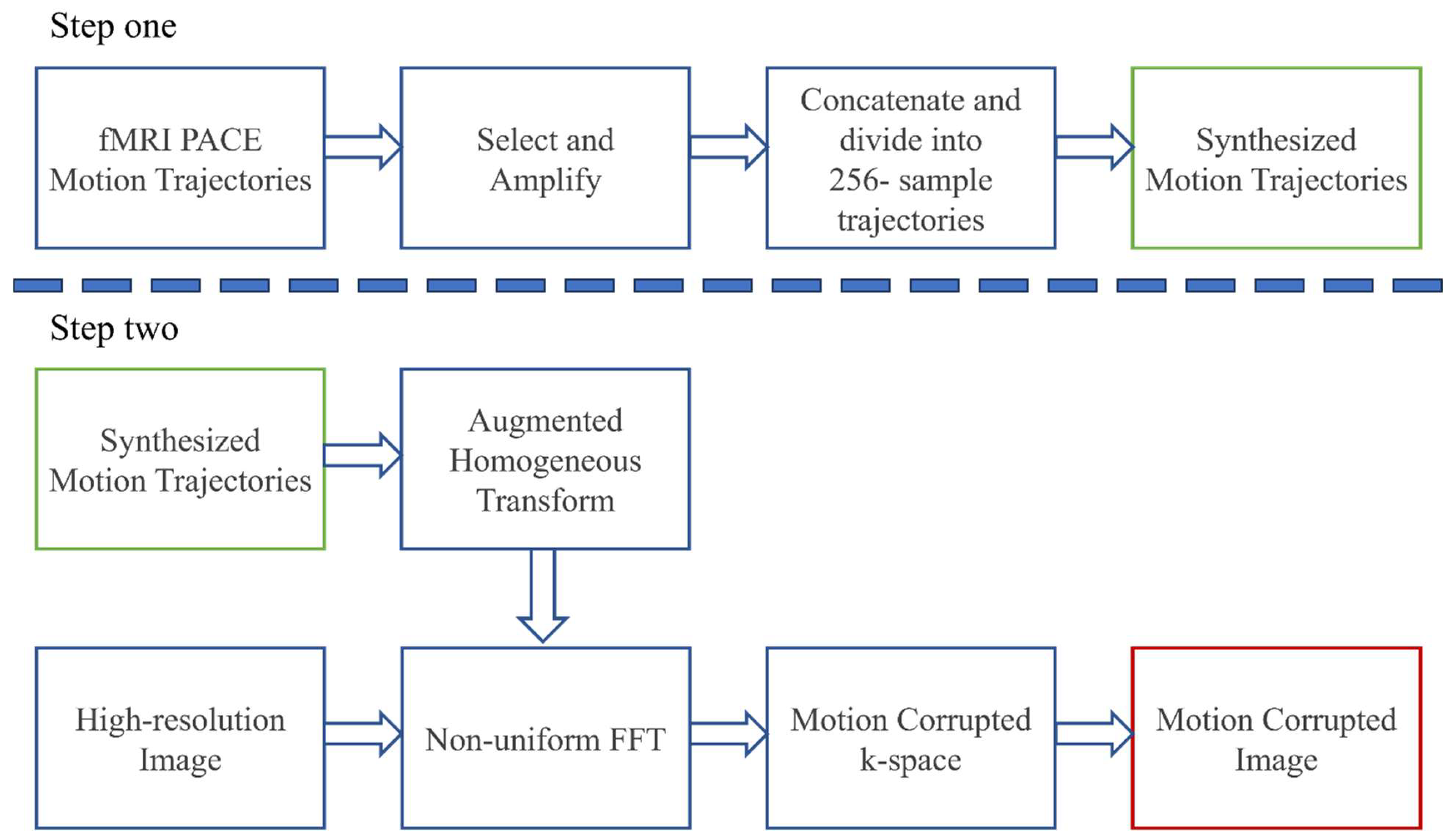
The pipeline of generating motion-corrupted images is shown in Figure 2. The (2D) source images were based on 3D sagittal magnetization-prepared rapid gradient-echo (MP-RAGE) scans and 2D axial fluid-attenuated inversion-recovery (FLAIR) scans obtained from 52 subjects and assessed visually to ensure they did not contain motion artifacts. The scan parameters for MP-RAGE were TR = 2.2 s; TE = 4.47 ms; TI = 1 s; resolution = 1 mm isotropic; and matrix size = 256 × 256 × 160, and those for FLAIR were TR = 9.1 s; TE = 84 ms; echo train length = 11; matrix size = 256 × 204; in-plane resolution = 1 mm2; slice thickness = 3 mm; slice spacing = 3 mm; and TI = 2.5 s.
Forty-two axial in-plane motion trajectories of 256 temporal samples each were generated from in vivo head movements measured with the prospective acquisition correction (PACE) algorithm [24] during BOLD functional MRI (fMRI). The source motion trajectories had translations < 2 mm and rotations < 2° and were subsequently multiplied by eight and reduced from 6 degrees of freedom to 3 in-plane motions (2 translations and 1 rotation). All motion trajectories were set to zero at the center of the trajectory (point 128). The severity of each motion trajectory applied is indicated by the temporal standard deviation for the three in-plane degrees of freedom (L2-norm of in-plane translations in mm and in-plane rotation in degrees).
To simulate motion artifacts, the original artifact-free 3D MP-RAGE images were zero-padded to 256 × 256 × 256, and sagittal as well as re-sliced axial and coronal 2D views were extracted. The resulting 2D images were then Fourier-transformed to create k-space data. Since rigid motion corrupts k-space data by changing the sampled k-space trajectory, the new k-space trajectory was calculated for each trajectory using the augmented homogeneous transform [8]. Next, the original (non-corrupted) k-space data were re-sampled on the motion k-space trajectory using non-uniform FFT (NuFFT) [25], and additional phase ramps induced by translations were added to obtain corrupted k-space data. Finally, motion-corrupted images were calculated via inverse Fourier-transformation of the corrupted k-space data.
Four different datasets were used. Datasets 1, 2, and 3 were generated with simulated motion, whereas dataset 4 contains images with real motion artifacts from human subjects.
Dataset 1 was used to train the neural network. Ten axial MP-RAGE slices spaced 5 mm apart were extracted from each “clean” (original) and corresponding motion-corrupted MP-RAGE volume. These images were divided into a training set (35 subjects; 25 motion trajectories; 13,700 slices), validation set (5 subjects; 7 motion trajectories; 1950 slices), and test set (12 subjects; 7 motion trajectories; 4680 slices). The subjects and motion trajectories in these sets did not overlap. As noted, motion trajectories for both training and testing data were magnified 8-fold.
Dataset 2 was used to test the generalizability of MC-Net with respect to unseen anatomical structures. It comprised motion-corrupted MP-RAGE images in sagittal (140 total slices) and coronal (140 total slices) views of 5 (of 12) subjects from the test set of Dataset 1.
Dataset 3 was used to test how well MC-Net adapts to a different type of image contrast without additional training. It consisted of 264 randomly selected motion-corrupted axial FLAIR images from 5 (of 12) healthy subjects from the test set of Dataset 1.
Dataset 4 was used for testing the MC-Net using data with real, rather than simulated, motion. It included a total of 15 T1-weighted images obtained from five subjects. The five subjects were not included in Dataset 1.

3.3. Quantitative Evaluation Metrics

The performance of the various methods employed was quantified using two measures. First, using the “clean” image as reference, the structural similarity index measure (SSIM) [26] was calculated:
S S I M ( x , y ) = ( 2 μ x μ y + C 1 ) ( 2 σ x y + C 2 ) ( μ x 2 + μ y 2 + C 1 ) ( σ x 2 + σ y 2 + C 2 )
where x and y are signals from input and reference, and μ x , μ y , σ x , σ y , and σ x y denote mean of input, mean of reference, variance of input, variance of reference, and covariance. C 1 and C 2 are two constants used to prevent the denominator from becoming zero.
The second performance measure was the peak-signal-to-noise ratio (PSNR). The PSNR is the ratio of the maximum possible power (MAX) of a signal and the power of distorting noise that affects the quality of its representation (i.e., the mean square error (MSE) between the denoising result from a DL model and the clean reference):
PSNR = 10 log 10 MAX 2 MSE
When the numerical difference between a predicted image and the reference approaches 0, the PSNR approaches infinity and the SSIM approaches 1.

3.4. Visual Reading Scores

The artifacts in the clean (reference) images, motion-corrupted images, MC-Net-predicted images, and L1-predicted images were assessed visually by three experienced imaging specialists who were blinded with respect to the correction method. The scores for image artifacts ranged from 0 to 3 (0 = “no”; 1 = “mild”; 2 = “moderate”; and 3 = “severe” motion artifacts). We also performed inter-rater evaluations of the three readers on the results of the UNet model trained with L1 only and the proposed MC-Net. Hence, we used the Pingouin open-source package [27] to calculate intraclass correlation coefficients (ICC) [28] and test–retest reliability (95% confidence intervals of ICC).
For simulated motion experiments, a mid-axial slice of five subjects from the test group were selected for reading. Ten distinct motion trajectories with a wide range of summed standard deviations were selected from the test group. The clean image, motion-corrupted image, and MC-Net prediction of each possible pair of a subject and a motion trajectory were reviewed by three imaging specialists in a randomized order. L1-norm prediction and MC-Net prediction were reviewed by the imaging specialists in a randomized order.
For the real (non-simulated) motion experiments, the motion-corrupted images, along with the MC-Net predictions of the five subjects in Dataset 4, were reviewed. Three slices were reviewed per subject, and motion artifacts were rated using the scale described above.
The artifact scores of motion-corrupted images and MC-Net predictions were compared using the one-sided Wilcoxon signed-rank test after averaging the reader scores. For simulated motions, artifact scores were compared for three ranges of summed standard deviations: [0–5] (mm/°), (6–10] (mm/°), and (10–15] (mm/°).

3.5. Implementation Details

All neural networks in this work were deployed in Keras [29], a deep learning programming platform built upon TensorFlow [30]. Our code supports Nifti image format. A workstation with an Intel Core™ i7-9700K CPU (3.60 GHZ, 64 GB RAM) and two Nvidia GeForce Titan 2080 GPUs was used. The overall process of operating MC-Net is shown in Algorithm 1.
Algorithm 1: The overall operation of training and testing MC-Net
Step 1:Initialize the weights of MC-Net (as shown in Figure 1) randomly,
Initialize variable for early stopping:
best_loss = infinity, counter = 0
Step 2:Define hyperparameters:
Learning rate, Number of epochs, and Batch size, Patience for early stopping.
Step 3:First stage training (L1 loss):
for each epoch from 1 to number of epochs do
   for each batch do
    Compute the predicted output using the current parameters
    Compute the loss between predicted and actual outputs
    Compute gradients of the loss with respect to the model parameters
    Update model parameters using ADAMS optimization algorithm
   Check for early stopping:
    If validation loss is less than best_loss
       Update best_loss = validation loss
       Reset counter = 0
    Else
       Increment counter
       If counter >= patience
         Exit training loop
Step 4:Second stage training (L1 + TV loss):
Take the MC-Net weight with best validation loss in Step 3 as initial weight.
Repeat the same procedure as in Step 3.
Step 5:Test the MC-Net:
Fed test images into the MC-Net and then get the outputs.
All models were trained in 200 epochs with a batch size of 8 on the training subset of Dataset 1. The ADAM optimizer [31] was selected to adapt the weights of each component to minimize the loss function during training, as suggested by [19]. We chose a learning rate of 0.0001 and a periodic decay of 0.96 after every epoch [2]. An early-stopping technique [32] was used during all the DL models’ training to avoid overfitting. We chose the epoch number of 200 heuristically, which ensures that the model can be sufficiently trained when we apply the early-stopping technique. We monitored validation loss during model training. If the validation loss did not show improvement after 10 epochs, we stopped the training process and saved the model with the best validation loss. We chose a batch size of 8 based on two considerations. First, a smaller batch size provided better model convergency in one study [33], and the model with a batch size of 8 performed better than a model with a batch size of 16. Second, batch sizes smaller than 8 will take substantially longer to train.
Experiments were performed using two slightly different network structures (Figure 1). The first experiment involved a conventional UNet structure (“U”) and was used to obtain the main results presented here, including those related to visual evaluation by clinicians. The other experiment involved an additional connection from input to output (“U + O”) to preserve more information from the input images [2] and was used for comparison with the “U” experiment. For comparison with the final MC-Net with the two-stage multi-loss function, single-stage models trained with the L1-loss [2] and with L1 + TV loss were also employed (“L1” and “L1 + TV” models).
Finally, since the mapping provided by DL algorithms is intrinsically non-linear, we performed an additional test to assess the preservation of information by feeding motion-free images into the various models and calculating the difference between the predicted results and the motion-free source images.

4. Results

The model used approximately 8.6 M parameters. Our final algorithm was able to process one image in 40 ms (on average) (GPU speed: approximately 32.7 G floating-point operations per second (FLOPS)).

4.1. Quantitative Improvements for Motion-Corrupted Images

Table 1 shows the SSIM (mean ± standard deviation (SD)) and PSNR (mean ± SD) values of the motion-corrected images compared to those for the uncorrected images in the test set of Dataset 1. The two-stage solution had the best performance among the three algorithms implemented (L1; L1 + TV; two-stage), although commonly only by a relatively small margin.
In comparison to the previously published UNet-like structure with optional input-to-output concatenation (“U + O”) [2], the proposed UNet solution (“Model U” in Table 1) showed significantly improved performance across the various methods (paired t-tests correspond to p < 0.005 for all contrasts). This difference was especially pronounced for the SSIM, which improved only marginally from 0.773 (corrupted images) to 0.816 (corrected images) for the U + O method with two stages while improving to 0.919 (corrected images) for the two-state algorithm without optional concatenation (U). Therefore, going forward, we will call the UNet algorithm with the two-stage multi-loss function but without optional concatenation the “MC-Net” algorithm.
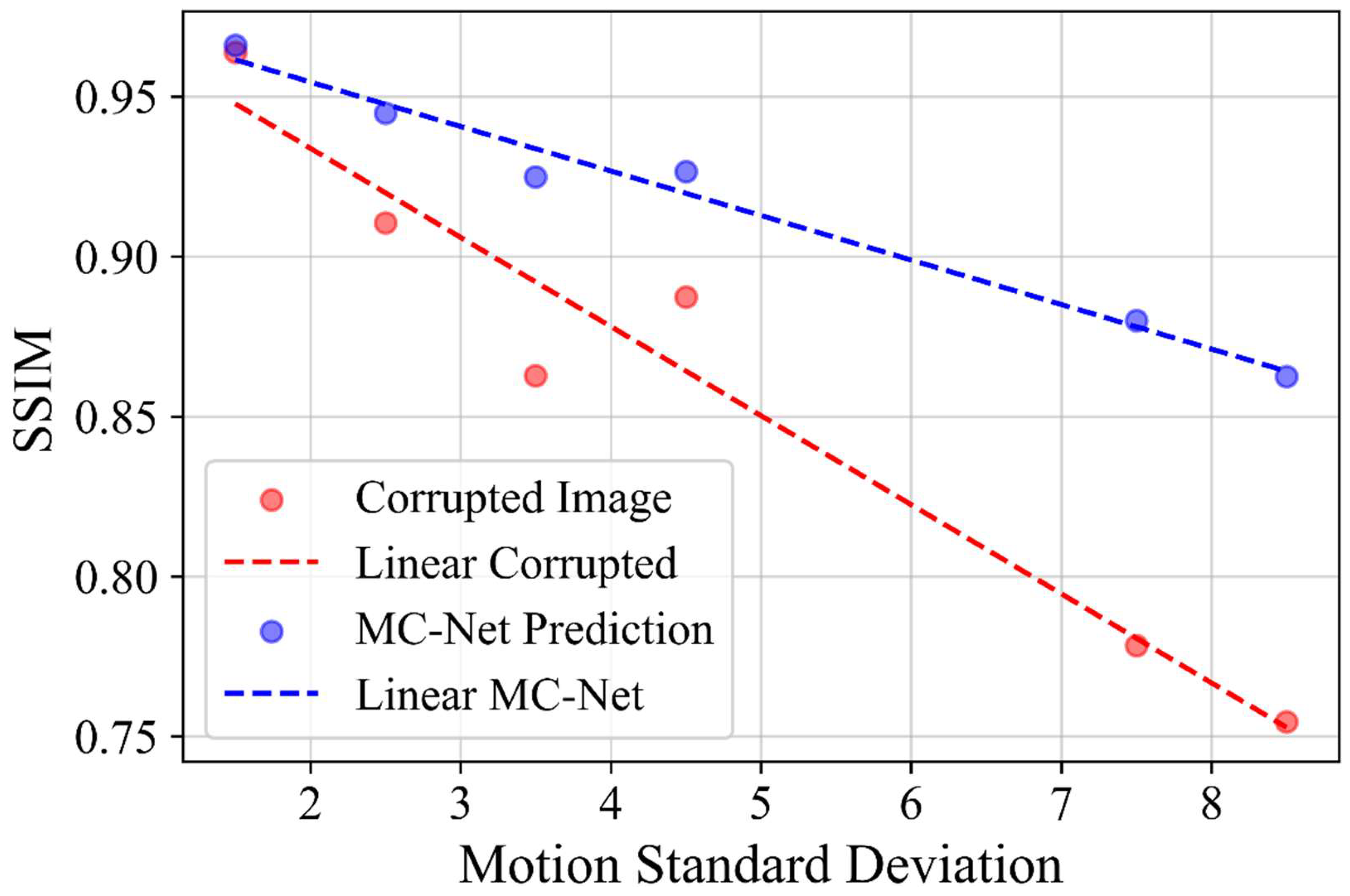
Figure 3 shows the relationship between the SSIM and the motion magnitude (defined as the standard deviation across 256 time points) for corrupted images and images corrected with the MC-Net algorithm. Without correction of motion artifacts, the SSIM decreases with the motion magnitude (from >0.95 for small motions below 1.5 mm/°) to approximately 0.75 for severe motion (with a slope of the linear regression curve = −0.028). MC-Net consistently improved image quality but was especially effective for large movements (slope = −0.014). Hence, the effect of motion on image quality decreased 2-fold (slope of regression line).

4.2. Effects on Artifact-Free Images

When artifact-free images were processed using the various networks, all algorithms generated high-quality images, with SSIMs consistently above 0.95 and almost 0.97 for the two-stage multi-loss function UNet (Table 2). Again, all differences in performance measures were significant at p < 0.005 (the SSIMs of the U + O network with L1, L1 + TV, and two-stage MC-Net seem identical because of rounding error).
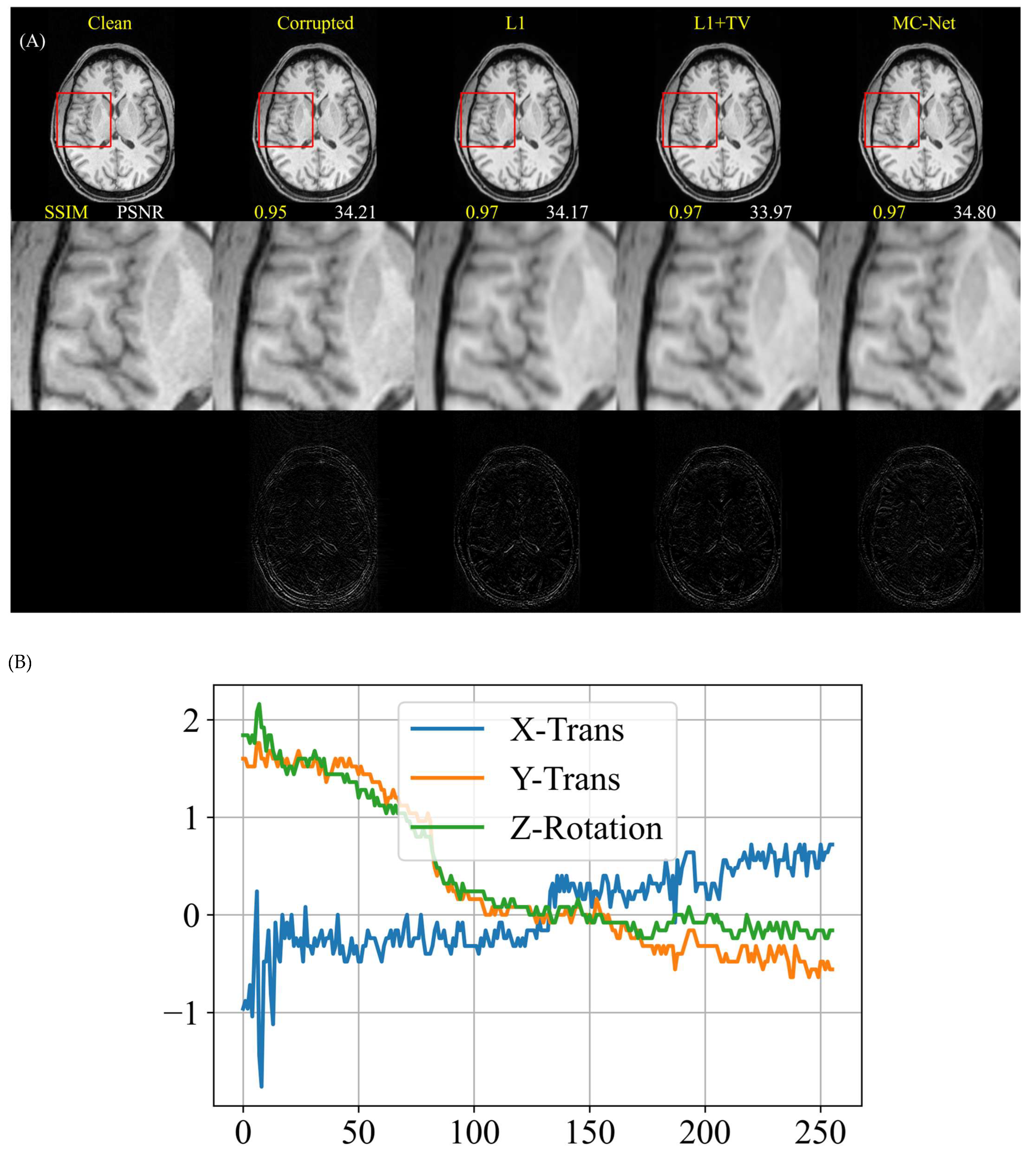
One example is shown in Figure 4, where the SSIM of a minimally corrupted image improves from 0.95 to 0.97 after processing using MC-Net was performed. However, the network with optional input-to-output concatenation achieved almost perfect agreement between the input and output images (SSIM > 0.99). Overall, MC-Net yielded the best performance for the correction of corrupted images while retaining the most information for “clean” images.

4.3. Visual Reading

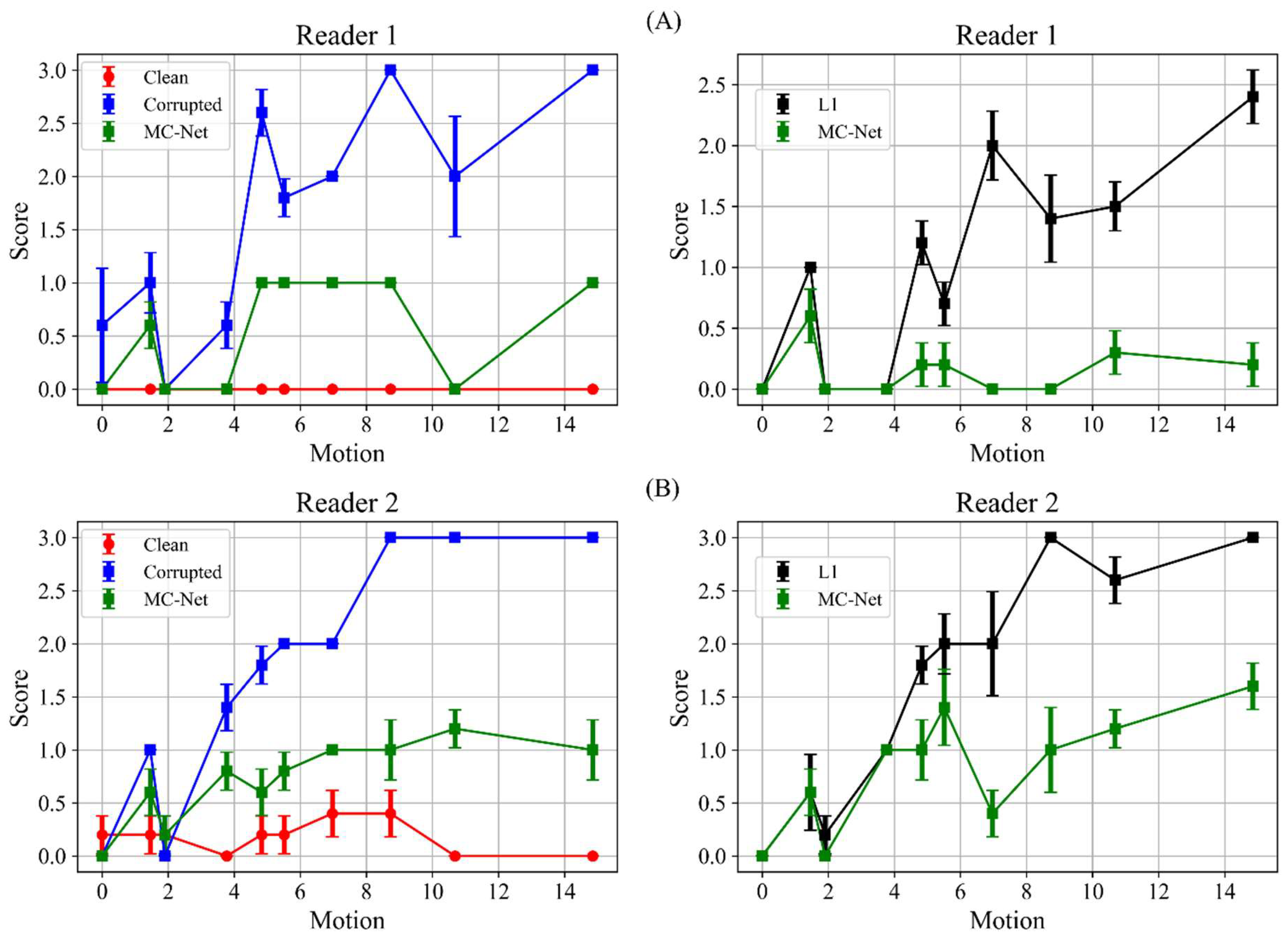
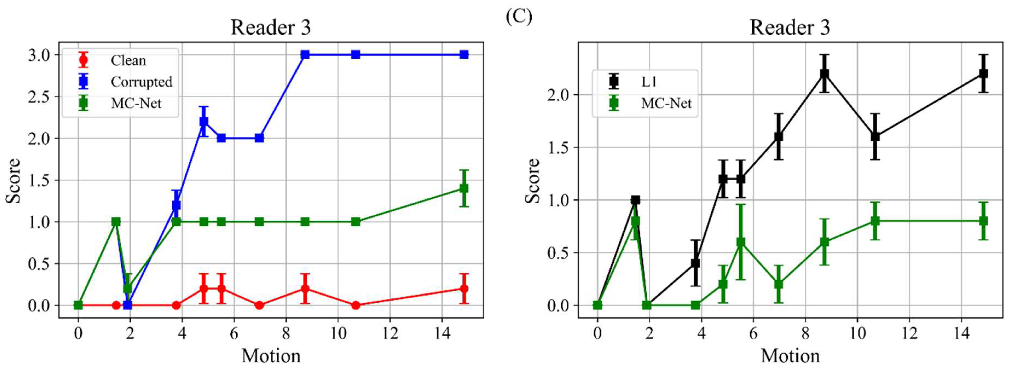
Figure 5 (left column) summarizes the readers’ visual assessments of reference images, motion-corrupted images, and the MC-Net predictions against the motion magnitude for 10 selected motions each for five subjects from the “test” data set (simulated movements). The “clean” reference images were consistently scored as showing no or only minor artifacts (red lines). Conversely, the scores of the corrupted images consistently worsened with the degree of motion such that most images with >7.5 mm/° motion (standard deviation across scan) were rated as having “moderate” or “severe” artifacts (blue lines). The visual scores of images processed using MC-Net improved significantly for motions from [0–5] mm/° (p = 5 × 10⁻⁴ on Wilcoxon signed-rank test), [5–10] mm/° (p = 6 × 10⁻⁵), and [10–15] mm/° (p = 2 × 10⁻³). Importantly, even images with the most severe ranges of simulated motion (>7.5 mm/°; green versus blue lines; left column) were rated to have only “minor artifacts” (on average) after correction.
Figure 5 (right column) demonstrates that MC-Net consistently outperformed the UNet model trained with L1-only in terms of visual image quality (paired t-tests across three raters: p = 0.009, p = 0.008, and p = 0.004). Based on the raters’ assessments, the test–retest reliability (ICC and 95% confidence intervals) values are 0.91 (0.86, 0.94) for L1 loss and 0.67 (0.5, 0.79) for MC-Net.
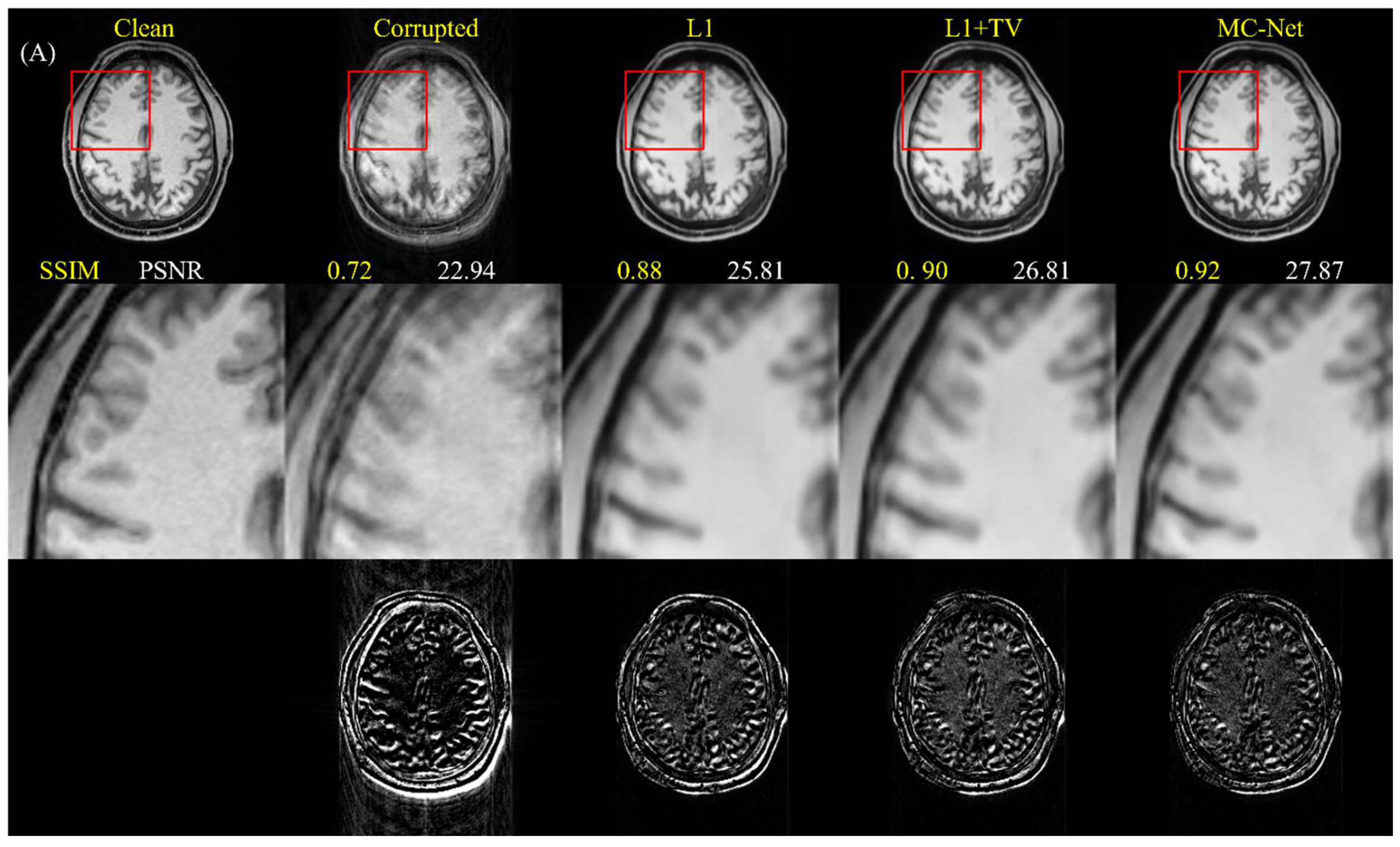
Representative results of the L1, L1 + TV, and MC-Net algorithms are shown in Figure 6. All DL methods improved image quality, but MC-Net was slightly more effective than the other methods. For instance, in an image with moderate motion artifacts (Figure 6A), MC-Net improved the SSIM from 0.72 to 0.92 and the PSNR from 22.9 to 27.9.
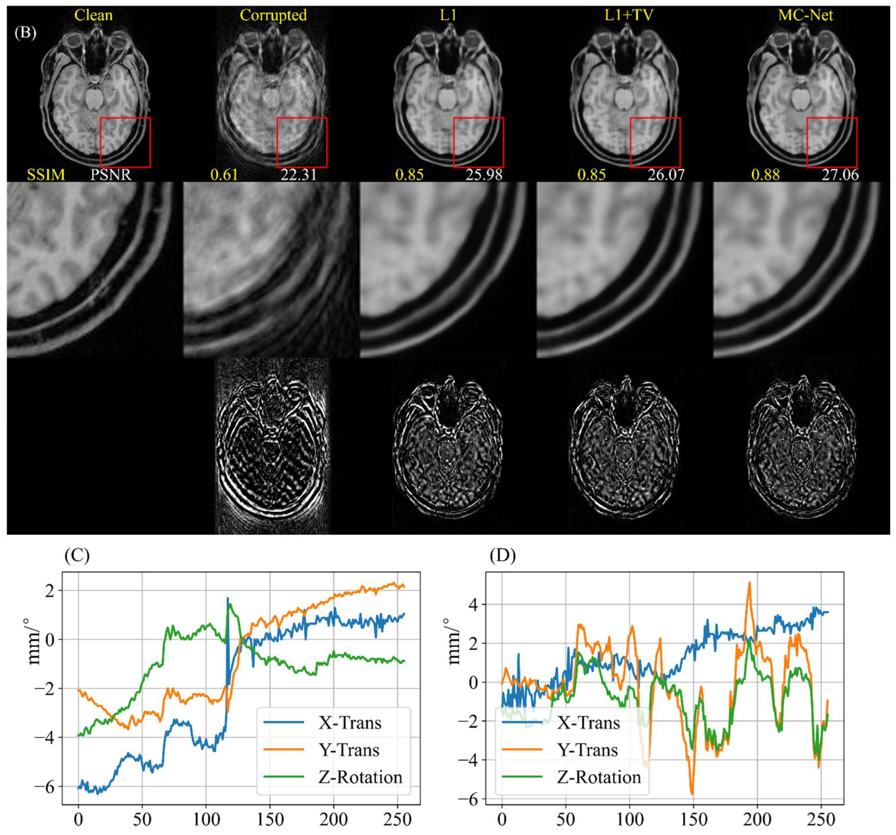
As an example, Figure 6B shows a representative image with severe motion artifacts. The corrupted image had an SSIM of 0.61 and a PSNR of 22.31 due to the severe movement simulated (a 10–15 mm/° sudden jump in the middle of the scan). After motion correction with MC-Net, the SSIM and PSNR improved to 0.88 and 27.06.
Of note, while motion artifacts were suppressed substantially after processing the images with originally moderate to severe artifacts, the corrected (output) images appeared to be processed with a low-pass filter. This contrasts with input images with little or no artifacts, where the low-pass effect was absent in the output images (e.g., Figure 4).

4.4. Cross-Dataset Generalization

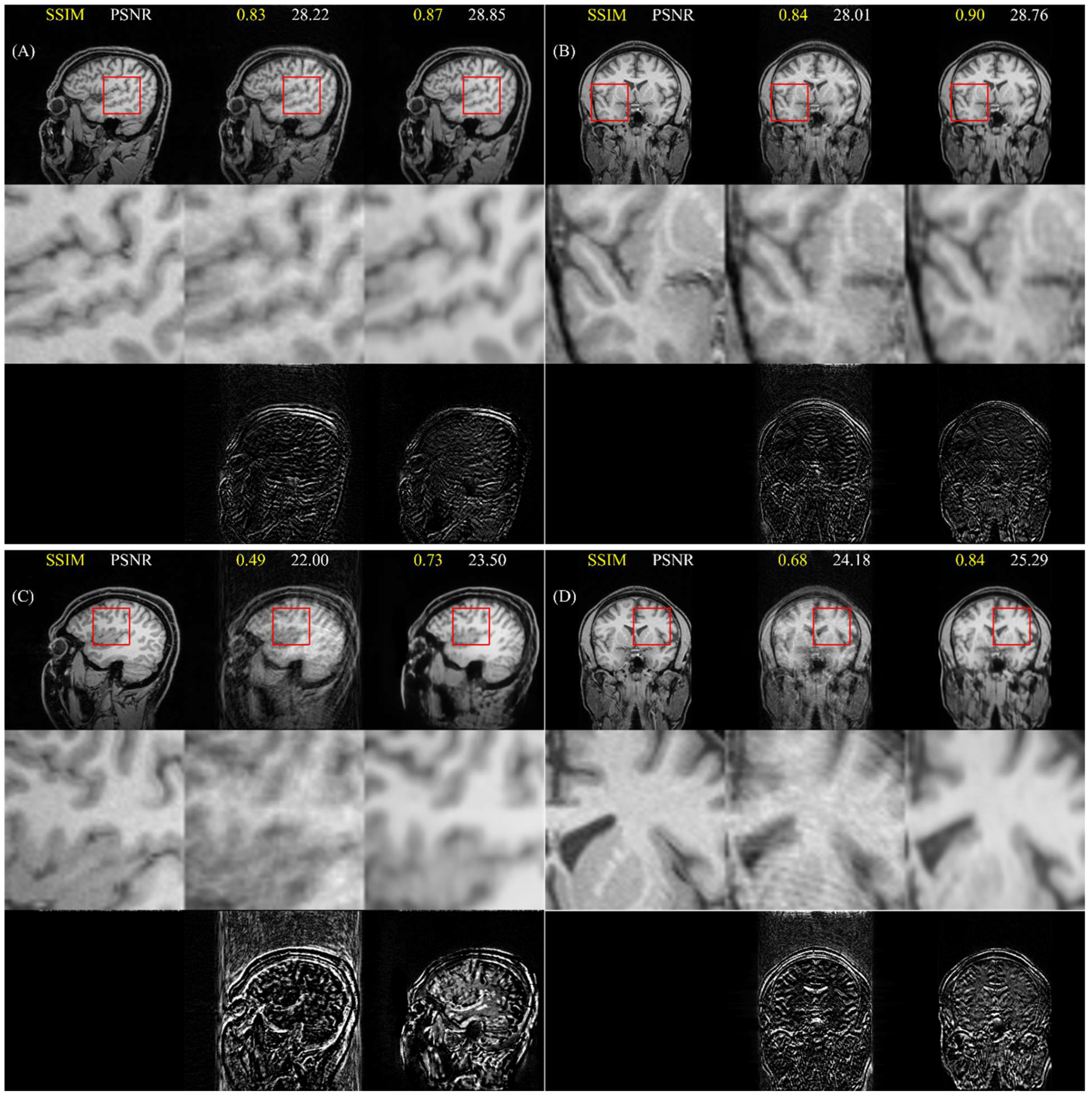
To assess cross-dataset generalization, we first applied the MC-Net algorithm (which was trained using axial images only) to sagittal and coronal T1-weighted slices with simulated motion artifacts. The mean SSIMs of sagital and coronal slices improved from 0.64 and 0.71 to 0.75 and 0.84, respectively. The mean PSNRs of sagital and coronal slices improved from 24.03 and 24.55 to 24.40 and 25.37, respectively. Representative results from two different scans are shown in Figure 7. The images from the first subject (Figure 7A,B; 3.95 mm/°) show mild to moderate motion artifacts. The SSIM values are similar for the two views, both before (0.83 and 0.84) and after the elimination of artifacts using MC-Net (0.87–0.9). The PSNR values for the two views are 28.22 and 28.01, and those after artifact removal using MC-Net are 28.85 and 28.76. The images from the second subject (Figure 7, bottom row; 5.99 mm/°) show moderate to severe motion artifacts, and the SSIM values improved from 0.49 to 0.73 (sagittal) and 0.68 to 0.84 (coronal). The PSNR values improved from 22.00 to 23.50 (sagittal) and 24.18 to 25.29 (coronal). Overall, these improvements in SSIM scores after processing with MC-Net are consistent with those observed for axial scans (regression lines in Figure 3).
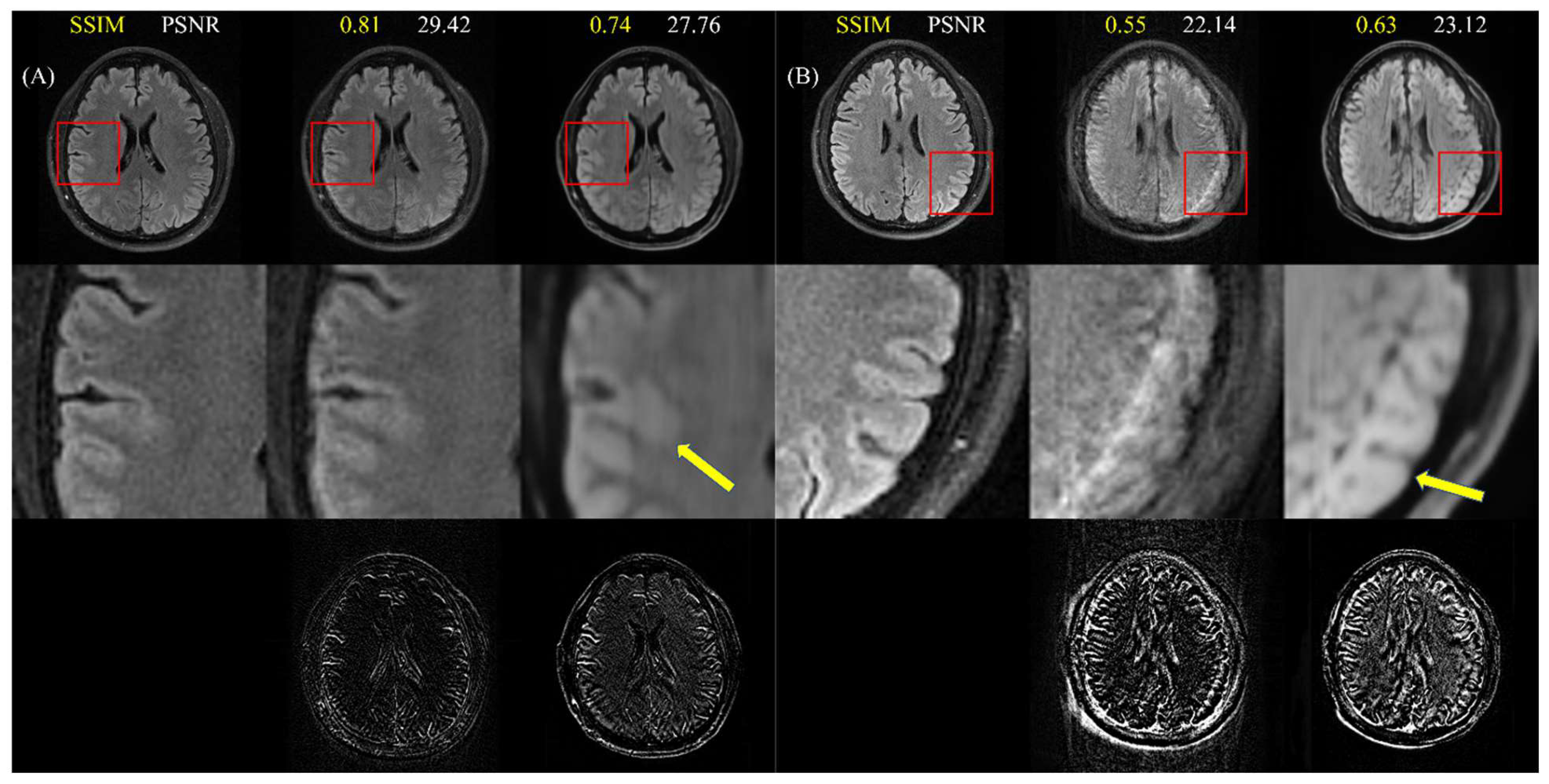
To assess the ability of the MC-Net algorithm to correct motion artifacts in T2-weighted images, we randomly selected and corrupted 264 slices with FLAIR contrast (Dataset 3). The SSIM and PSNR of the corrupted images were 0.69 ± 0.11 and 26.15 ± 2.72 (mean ± SD), and they were 0.67 ± 0.04 and 25.25 ± 1.54 after correction. Thus, processing with MC-Net slightly decreased image quality. This finding was confirmed visually based on two axial slices from two different subjects (Figure 8) using simulated motion artifacts. In the first set of images (Figure 8A) with relatively minor motion (3.77 mm/°), the SSIM and PSNR values were poorer after the images were processed using MC-Net, and slight banding artifacts appeared. Conversely, when MC-Net was applied to a FLAIR image with more-severe motion artifacts (Figure 8B, 14.85 mm/°), the SSIM and PSNR values improved (from 0.55 to 0.63 and from 22.14 to 23.12, respectively). However, despite these apparent improvements, the highlighted region of the “corrected” image provides a poor representation of the original scan; in fact, new (false) anatomical “features” appear in the “corrected” image.

4.5. Images with Real (Non-Simulated) Motion

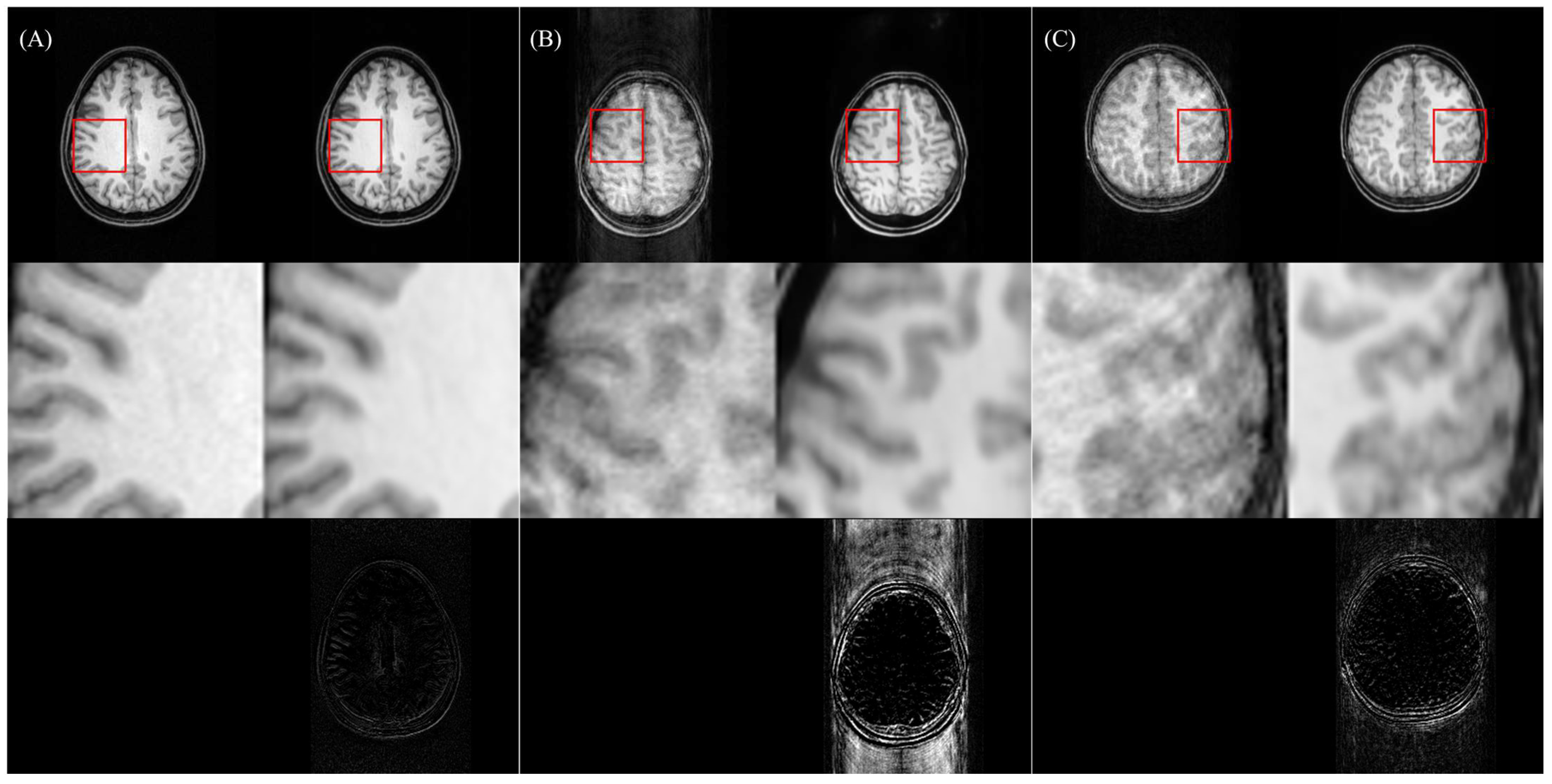
As a final validation step, we applied the MC-Net algorithm to human brain images with various degrees of motion artifacts (not simulated). Some representative results are shown in Figure 9, with the apparent degree of motion corruption increasing from Figure 9A–C. As before, the image with minor motion artifacts Figure 9A was well preserved by MC-Net, whereas the two scans with moderate and severe artifacts, Figure 9B,C, showed substantial improvements in quality after being processed by MC-Net. While it is obvious that no reference images are available for quantifying improvements in image quality, the visual image scores provided by our blinded readers improved significantly between the original and corrected scans (p = 0.04).

5. Discussion

The goal of our work was to develop a DL-based automated method for eliminating or attenuating motion artifacts in brain MRI scans. The resulting MC-Net network uses a novel loss function and a novel training strategy and was trained and tested using data involving a wide range of real movements. A series of comprehensive evaluations were performed to assess the risk of over-correction and generalizability. The former was assessed by inputting the motion-free images and assessing how well the quality of images was preserved after being processed by MC-Net. The latter was assessed through testing MC-Net on a different dataset with different image orientations and image contrasts.
As in previous work [2,9,34], MC-Net was able to correct motion artifacts in brain scans. We based our work on a customized UNet-like auto-encoder architecture [35] that is widely used in medical image analysis. This network architecture is complex enough to perform motion correction but also simple enough to benefit from the hybrid loss function. The proposed hybrid loss and two-stage training was slightly better in terms of improving final image quality than approaches with single-stage training, e.g., the L1 loss used in a prior study [2], and was especially beneficial for correcting severe motion artifacts. Due to the short processing time per image (40 ms), implementation using the open-source framework Keras [29] with GPU acceleration should allow real-time motion correction.
We base the comparison of our results to those from other studies on the SSIM, since it is commonly used to assess the performance of deep learning algorithms for brain/head MRI motion correction. Also, it is important to consider that SSIM values and improvements are dependent upon the degree of motion corruption (Figure 3). The first comparison paper [34] had pre- and post-correction SSIM values of 0.863 (suggesting moderate motion) and 0.924; the improvement approximately matches that of MC-Net. The second comparison paper [19] reports SSIM values of 0.795 (corrupted) and 0.862 (corrected), suggesting an improvement somewhat below that achievable with MC-Net (based on the linear regressions in Figure 3). Finally, a third paper [1] found an improvement in SSIM from 0.68 to 0.92. The pre-correction value of 0.68 suggests substantial motion artifacts and is in fact outside the range assessed by our simulations (lowest value is 0.75). Overall, the improvement in SSIM between the motion-corrupted images (0.773) and the motion-corrected results (0.919) from MC-Net is better than that of the first two studies but smaller than that achieved by the model proposed in [1]. The greater improvement of the model may be a result of integrating the pre-trained VGG [36] as a main building block of the DL model. By using the pre-trained VGG, the DL model can benefit from transfer learning, which has been shown to boost performance for other medical imaging or computer vision tasks, such as in [10,13,14,37]. Conversely, we trained our initial model from scratch.

5.1. Advantages of Two-Stage Training and Multiple-Loss Function

Two-stage training can distill different information at each stage and benefit applications such as the reconstruction of high-resolution arterial spin-labeling MRI [38] and image denoising [39]. We observed that the first L1 stage could recreate the overall anatomical structure, but some fine details were missing when large movements were simulated. Inspired by the style transfer approach [23,40], we added the total variation term to remove residual artifacts and introduce smoothness across pixels. As a result, it was observed that MC-Net is slightly better than the multi-loss method with single-stage training, perhaps since a model trained in only one stage may fall into a local minimum, a problem that the second stage training step might have avoided.

5.2. Comparison of Different DL Architectures

We tested two different architectures, i.e., UNet-like (U) and UNet-like plus an additional input-to-output connection (U + O) as suggested in prior work [2]. Interestingly, the simpler U-model yielded better SSIM and PSNR values than the U + O model for motion-corrupted images. We conjecture that the input-to-output connection passes too much original context information (noise and artifacts included) to the output, degrading the results. Therefore, the U-architecture with the two-stage multiple-loss method had the overall best performance for both motion-corrupted and motion-free images.
All three U + O models [2] performed almost perfectly in terms of SSIM for motion-free images (with an SSIM of essentially 1.0), independent of which loss function was used during training. This is likely a result of the additional input-to-output connection in the U + O model, which allowed the passing of more information from the original image to the output compared with the U model. This additional information made the results from U + O more like the motion-free image.
However, amongst the U-models, the model trained with the two-stage multiple-loss method still had the best PSNR for motion-free images, which demonstrates that the two-stage multiple-loss method may be applied widely to different DL architectures.

5.3. Performance on Test Set

MC-Net achieved promising results on corrupted axial test datasets with T1-contrast both in terms of SSIM and PSNR. In addition, the visual quality scores provided by two experienced imaging specialists demonstrate that MC-Net can attenuate motion artifacts and improve image quality.

5.4. Cross-Dataset Generalization

Our DL model was trained with a single orientation (axial) and contrast (T1-weighting using MP-RAGE). Therefore, we assessed the generalizability of MC-Net using datasets with untrained orientations and untrained contrast. In terms of new orientations (sagittal and coronal) without change in contrast (T1), the quantitative improvements in image quality after processing with the MC-Net were similar to those for the trained orientation (axial) for a given number of motion artifacts. Importantly, MC-Net also improved the quality of actual T1-weighted images that were corrupted during acquisition. However, neither MC-Net nor the network with an additional input–output connection markedly improved the visual quality of clinical images. This is most likely because the training data set did not include clinical images and since the clinical images showed less gray-white matter contrast than the training data.
MC-Net provided little to no benefit in terms of correcting motion artifacts in axial T2 view images. Therefore, image contrast appears to have more relevance in representing imaging artifacts than anatomical structure. Hence, motion correction may be considered a low-level vision problem in which a low-level clue (contrast) is more important than a high-level clue (anatomical structure).
Compared with previous studies using DL to correct motion-induced artifacts, our paper contains a comprehensive and in-depth assessment of the performance of MC-Net. In addition to quantitative measures such as SSIM and PSNR, the severity of motion artifacts was assessed by imaging specialists and analyzed statistically. The motion trajectories in the simulated motion experiments span a wide range of severity and were synthesized from real recorded motion trajectories in exams. MC-Net was tested for cross-dataset generalization with respect to the image contrast and with respect to the anatomical structures, which change with image orientation.

5.5. Limitations

While we attempted to perform a comprehensive evaluation of the proposed MC-Net, our study also has several limitations. First, the range of imaging contrasts evaluated was focused on T1-weighted, more specifically MP-RAGE, and a few T2-weighted scans (FLAIR). Therefore, we do not know how our model performs for other contrasts, such as susceptibility weighted or conventional T2-weighted contrast. However, given the poor performance of MC-Net in processing FLAIR images, it is likely that the current network would not be beneficial for other contrasts either.
Second, we did not include sagittal or coronal data in the training set or evaluate the corresponding performance since we focused on a scenario where only one source of data is available and sufficient to train the model, i.e., single-domain generalization [41]. These factors might be relevant in the clinical setting. We plan to include sagittal and coronal data to train the model for more comprehensive evaluation in the near future.
The motion trajectories used in this work were based on real head motions measured with PACE-fMRI and are more realistic compared with options such as sinusoids and other regular patterns or random motion trajectories. However, the time scale of the motion trajectories was not resampled to match that of the MP-RAGE and FLAIR acquisitions. Consequently, movements in the simulations were to some degree slowed down or accelerated compared with the PACE measurements. Further, the amplitude of movements was magnified to create more challenging artifacts for MC-Net. Therefore, some degree of authenticity of the motion trajectories was sacrificed for higher temporal resolution and higher motion amplitudes. Also, the simulation of motion artifacts did not include the effects of movements on spin saturation across TR-periods. However, since MP-RAGE is a 3D acquisition, the spin-history effects are probably relatively minor; we did not model through-plane motion.
It is worth noting that this model was not trained and tested for extremely large motions. Extreme cases can be added by fine-tuning the model with new training samples and intermediate samples, possibly to be generated using a Projection-On-Convex-Set-based cycle Generative Adversarial Network [11].

6. Conclusions

In conclusion, we developed a simulation framework and MC-Net for the correction of motion artifacts in brain MRI images. The MC-Net performed well on unseen data and images of different orientations with the same contrast (T1-weighted), but scans with other types of contrast will require additional optimizations. The high reader scores and evaluation metrics of the corrected images demonstrate the viability of MC-Net for correcting motion artifacts. Since this method is data-driven and independent of data acquisition or reconstruction and can be quickly performed, it may ultimately be suitable for routine clinical practice. In the future, we plan to improve the performance of MC-Net for other contrasts and may employ MC-Net using vision transformers (ViT) [21,42].

Author Contributions

Conceptualization, T.E. and Z.W.; Methodology, L.Z., X.W. and Z.W.; Software, L.Z. and X.W.; Validation, L.C., E.H.H. and E.R.M.; Formal Analysis, M.R. and R.B; Investigation, Z.W. and T.E.; Resources, T.E.; Data Curation, X.W.; Writing—Original Draft Preparation, L.Z.; Writing—Review & Editing, T.E. and Z.W.; Visualization, L.Z. and X.W.; Supervision, T.E. and Z.W.; Project Administration, T.E.; Funding Acquisition, T.E., R.B. and Z.W. All authors have read and agreed to the published version of the manuscript.

Funding

This work was supported by NIH grant 1R01 DA021146 (BRP), R01AG060054, R01AG070227, R01EB031080-01A1, P41EB029460-01A1, R01AG081693, R01EB031080, P41EB029460, R21AG080518, and 1UL1TR003098. M.R. and R.B. were supported in part by NSF grant DMS-2108900 and Simons Foundation Fellowship grant 818333.

Data Availability Statement

Restrictions apply to the datasets: The datasets presented in this article are not readily available because the research participants did not provide explicit consent for data sharing. Requests for accessing the datasets should be directed to Thomas Ernst.

Conflicts of Interest

The authors declare no conflicts of interest.

References

  1. Küstner, T.; Armanious, K.; Yang, J.; Yang, B.; Schick, F.; Gatidis, S. Retrospective correction of motion-affected MR images using deep learning frameworks. Magn. Reson. Med. 2019, 82, 1527–1540. [Google Scholar] [CrossRef]
  2. Pawar, K.; Chen, Z.; Shah, N.J.; Egan, G.F. Suppressing motion artefacts in MRI using an Inception-ResNet network with motion simulation augmentation. NMR Biomed. 2019, 35, e4225. [Google Scholar] [CrossRef]
  3. Andre, J.B.; Bresnahan, B.W.; Mossa-Basha, M.; Hoff, M.N.; Smith, C.P.; Anzai, Y.; Cohen, W.A. Toward quantifying the prevalence, severity, and cost associated with patient motion during clinical MR examinations. J. Am. Coll. Radiol. 2015, 12, 689–695. [Google Scholar] [CrossRef]
  4. Skare, S.; Hartwig, A.; Mårtensson, M.; Avventi, E.; Engström, M. Properties of a 2D fat navigator for prospective image domain correction of nodding motion in brain MRI. Magn. Reson. Med. 2015, 73, 1110–1119. [Google Scholar] [CrossRef]
  5. Wallace, T.E.; Afacan, O.; Waszak, M.; Kober, T.; Warfield, S.K. Head motion measurement and correction using FID navigators. Magn. Reson. Med. 2019, 81, 258–274. [Google Scholar] [CrossRef]
  6. Zaitsev, M.; Maclaren, J.; Herbst, M. Motion artifacts in MRI: A complex problem with many partial solutions. J. Magn. Reson. Imaging 2015, 42, 887–901. [Google Scholar] [CrossRef]
  7. Maclaren, J.; Herbst, M.; Speck, O.; Zaitsev, M. Prospective motion correction in brain imaging: A review. Magn. Reson. Med. 2013, 69, 621–636. [Google Scholar] [CrossRef]
  8. Zahneisen, B.; Ernst, T. Homogeneous coordinates in motion correction. Magn. Reson. Med. 2016, 75, 274–279. [Google Scholar] [CrossRef]
  9. Usman, M.; Latif, S.; Asim, M.; Lee, B.-D.; Qadir, J. Retrospective motion correction in multishot MRI using generative adversarial network. Sci. Rep. 2020, 10, 4786. [Google Scholar] [CrossRef]
  10. Zhou, Z.; Shin, J.; Zhang, L.; Gurudu, S.; Gotway, M.; Liang, J. Fine-tuning convolutional neural networks for biomedical image analysis: Actively and incrementally. In Proceedings of the IEEE Conference on Computer Vision and Pattern Recognition, Honolulu, HI, USA, 21–26 July 2017; pp. 7340–7351. [Google Scholar]
  11. Li, Y.; Yang, H.; Xie, D.; Dreizin, D.; Zhou, F.; Wang, Z. POCS-Augmented CycleGAN for MR Image Reconstruction. Appl. Sci. 2021, 12, 114. [Google Scholar] [CrossRef]
  12. Xie, D.; Li, Y.; Yang, H.; Bai, L.; Wang, T.; Zhou, F.; Zhang, L.; Wang, Z. Denoising arterial spin labeling perfusion MRI with deep machine learning. Magn. Reson. Imaging 2020, 68, 95–105. [Google Scholar] [CrossRef]
  13. Zhang, L.; Xie, D.; Li, Y.; Camargo, A.; Song, D.; Lu, T.; Jeudy, J.; Dreizin, D.; Melhem, E.R.; Wang, Z.; et al. Improving Sensitivity of Arterial Spin Labeling Perfusion MRI in Alzheimer’s Disease Using Transfer Learning of Deep Learning-Based ASL Denoising. J. Magn. Reson. Imaging 2022, 55, 1710–1722. [Google Scholar] [CrossRef]
  14. Zhang, L.; Mohamed, A.A.; Chai, R.; Guo, Y.; Zheng, B.; Wu, S. Automated deep learning method for whole-breast segmentation in diffusion-weighted breast MRI. J. Magn. Reson. Imaging 2020, 51, 635–643. [Google Scholar] [CrossRef]
  15. Zhang, L.; Arefan, D.; Guo, Y.; Wu, S. Fully automated tumor localization and segmentation in breast DCEMRI using deep learning and kinetic prior. In Proceedings of the Medical Imaging 2020: Imaging Informatics for Healthcare, Research, and Applications, Houston, TX, USA, 16–17 February 2020; Volume 11318, p. 113180Z. [Google Scholar]
  16. Balakrishnan, G.; Zhao, A.; Sabuncu, M.R.; Guttag, J.; Dalca, A.V. VoxelMorph: A learning framework for deformable medical image registration. IEEE Trans. Med. Imaging 2019, 38, 1788–1800. [Google Scholar] [CrossRef]
  17. Dalca, A.V.; Balakrishnan, G.; Guttag, J.; Sabuncu, M.R. Unsupervised learning of probabilistic diffeomorphic registration for images and surfaces. Med. Image Anal. 2019, 57, 226–236. [Google Scholar] [CrossRef]
  18. Johnson, P.M.; Drangova, M. Conditional generative adversarial network for 3D rigid-body motion correction in MRI. Magn. Reson. Med. 2019, 82, 901–910. [Google Scholar] [CrossRef]
  19. Hossbach, J.; Splitthoff, D.N.; Cauley, S.; Clifford, B.; Polak, D.; Lo, W.-C.; Meyer, H.; Maier, A. Deep learning-based motion quantification from k-space for fast model-based magnetic resonance imaging motion correction. Med. Phys. 2022, 50, 2148–2161. [Google Scholar] [CrossRef]
  20. Beljaards, L.; Pezzotti, N.; Rao, C.; Doneva, M.; van Osch, M.J.P.; Staring, M. AI-based motion artifact severity estimation in undersampled MRI allowing for selection of appropriate reconstruction models. Med. Phys. 2024, 51, 3555–3565. [Google Scholar] [CrossRef]
  21. Spieker, V.; Eichhorn, H.; Hammernik, K.; Rueckert, D.; Preibisch, C.; Karampinos, D.C.; Schnabel, J.A. Deep learning for retrospective motion correction in MRI: A comprehensive review. IEEE Trans. Med. Imaging 2023, 43, 846–859. [Google Scholar] [CrossRef]
  22. Zhang, L.; Luo, Z.; Chai, R.; Arefan, D.; Sumkin, J.; Wu, S. Deep-learning method for tumor segmentation in breast DCE-MRI. In Proceedings of the Medical Imaging 2019: Imaging Informatics for Healthcare, Research, and Applications, San Diego, CA, USA, 17–18 February 2019; Volume 10954, p. 109540F. [Google Scholar]
  23. Chollet, F. Deep Learning with Python; Manning: New York, NY, USA, 2018; Volume 361. [Google Scholar]
  24. Thesen, S.; Heid, O.; Mueller, E.; Schad, L.R. Prospective acquisition correction for head motion with image-based tracking for real-time fMRI. Magn. Reson. Med. 2000, 44, 457–465. [Google Scholar] [CrossRef]
  25. Greengard, L.; Lee, J.-Y. Accelerating the nonuniform fast Fourier transform. SIAM Rev. 2004, 46, 443–454. [Google Scholar] [CrossRef]
  26. Wang, Z.; Bovik, A.C.; Sheikh, H.R.; Simoncelli, E.P. Image quality assessment: From error visibility to structural similarity. IEEE Trans. Image Process. 2004, 13, 600–612. [Google Scholar] [CrossRef]
  27. Vallat, R. Pingouin: Statistics in Python. J. Open Source Softw. 2018, 3, 1026. [Google Scholar] [CrossRef]
  28. Shrout, P.E.; Fleiss, J.L. Intraclass correlations: Uses in assessing rater reliability. Psychol. Bull. 1979, 86, 420. [Google Scholar] [CrossRef]
  29. Chollet, F. Keras. GitHub. 2015. Available online: https://github.com/fchollet/keras (accessed on 11 November 2021).
  30. Abadi, M.; Barham, P.; Chen, J.; Chen, Z.; Davis, A.; Dean, J.; Devin, M.; Ghemawat, S.; Irving, G.; Isard, M.; et al. Tensorflow: A system for large-scale machine learning. In Proceedings of the 12th USENIX Conference on Operating Systems Design and Implementation, Savannah, GA, USA, 2–4 November 2016; pp. 265–283. [Google Scholar]
  31. Kingma, D.P.; Ba, J. Adam: A method for stochastic optimization. arXiv 2014, arXiv:1412.6980. [Google Scholar]
  32. Prechelt, L. Early stopping-but when? In Neural Networks: Tricks of the Trade; Springer: Berlin/Heidelberg, Germany, 1998; pp. 55–69. [Google Scholar]
  33. Keskar, N.S.; Nocedal, J.; Tang, P.T.P.; Mudigere, D.; Smelyanskiy, M. On large-batch training for deep learning: Generalization gap and sharp minima. arXiv 2016, arXiv:1609.04836. [Google Scholar]
  34. Sommer, K.; Saalbach, A.; Brosch, T.; Hall, C.; Cross, N.M.; Andre, J.B. Correction of motion artifacts using a multiscale fully convolutional neural network. Am. J. Neuroradiol. 2020, 41, 416–423. [Google Scholar] [CrossRef]
  35. Ronneberger, O.; Fischer, P.; Brox, T. U-net: Convolutional networks for biomedical image segmentation. In Proceedings of the International Conference on Medical Image Computing and Computer-Assisted Intervention, Munich, Germany, 5–9 October 2015; pp. 234–241. [Google Scholar]
  36. Simonyan, K.; Zisserman, A. Very deep convolutional networks for large-scale image recognition. arXiv 2014, arXiv:1409.1556. [Google Scholar]
  37. Yang, F.; Zhang, L.; Yu, S.; Prokhorov, D.; Mei, X.; Ling, H. Feature pyramid and hierarchical boosting network for pavement crack detection. IEEE Trans. Intell. Transp. Syst. 2019, 21, 1525–1535. [Google Scholar] [CrossRef]
  38. Li, Z.; Liu, Q.; Li, Y.; Ge, Q.; Shang, Y.; Song, D.; Wang, Z.; Shi, J. A two-stage multi-loss super-resolution network for arterial spin labeling magnetic resonance imaging. In Proceedings of the International Conference on Medical Image Computing and Computer-Assisted Intervention, Shenzhen, China, 13–17 October 2019; pp. 12–20. [Google Scholar]
  39. Wu, X.; Liu, M.; Cao, Y.; Ren, D.; Zuo, W. Unpaired learning of deep image denoising. In Proceedings of the European Conference on Computer Vision, Glasgow, UK, 23–28 August 2020; pp. 352–368. [Google Scholar]
  40. Gatys, L.A.; Ecker, A.S.; Bethge, M. A neural algorithm of artistic style. arXiv 2015, arXiv:1508.06576. [Google Scholar] [CrossRef]
  41. Qiao, F.; Zhao, L.; Peng, X. Learning to learn single domain generalization. In Proceedings of the IEEE/CVF Conference on Computer Vision and Pattern Recognition, Seattle, WA, USA, 14–19 June 2020; pp. 12556–12565. [Google Scholar]
  42. Shamshad, F.; Khan, S.; Zamir, S.W.; Khan, M.H.; Hayat, M.; Khan, F.S.; Fu, H. Transformers in medical imaging: A survey. Med. Image Anal. 2023, 88, 102802. [Google Scholar] [CrossRef]
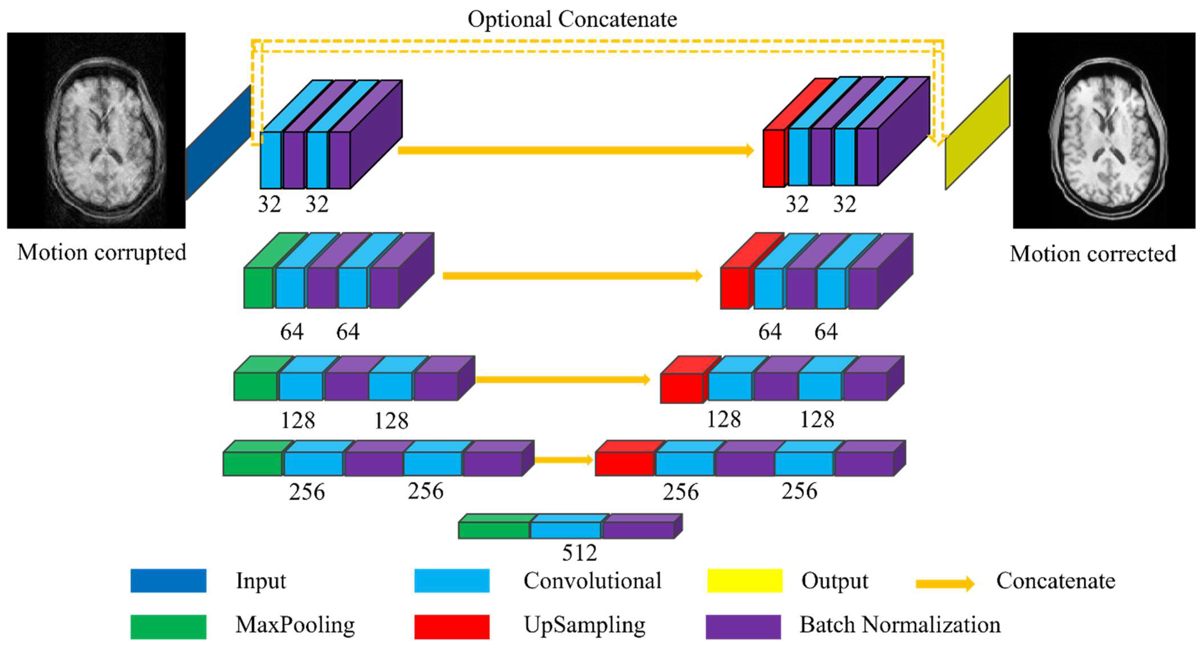
Figure 1. Architecture of MC-Net, which was derived from UNet. The filter number in each convolutional layer of the customized UNet is half that of the original UNet [22]. An optional concatenation on top of the UNet structure is indicated by a dashed line.
Algorithms 17 00215 g001
Figure 2. The pipeline corresponding to generating motion-corrupted k-space data. Step 1 describes the synthesis of motion trajectories. Step 2 shows how motion corrupted images are generated using motion trajectories and high-resolution images as input.
Algorithms 17 00215 g002
Figure 3. SSIM values of images corrected with MC-Net (blue dots) relative to those of uncorrupted images (red dots) are plotted against the magnitude of motion simulated (standard deviation of motion across 256 time points, in mm/°). The red line (Y = 0.99 − 0.028X) and blue line (Y = 0. 98 − 0.014X) show linear regression of images without and with motion correction against the motion magnitude.
Algorithms 17 00215 g003
Figure 4. Examples of motion artifact removal from images in the test data set of Dataset 1 using various algorithms. In (A) (1.90 mm/°), the first row contains the clean reference image, corrupted image, and motion correction results using the L1, L1 + TV, and MC-Net algorithms. The second row shows an enlarged image of the red rectangle. The SSIM and PSNR values for each corrected image (relative to the “clean” image) are also shown (bottom row). The third row shows the error maps between the reference (i.e., clean image) and corrupted image and motion correction results. The difference between each pixel shown in the error maps was multiplied by a factor of five. (B) The motion trajectory for (A), where the horizontal axis labels refer to y-position in k-space.
Algorithms 17 00215 g004
Figure 5. Average motion artifact scores of test data set of Dataset 1 made by three blinded clinical readers (top to bottom for reader 1 (A), reader 2 (B) and reader 3 (C)) as a function of motion magnitude (x-axis). The left column shows visual scores for “clean” reference images (red lines), motion-corrupted images (blue lines), and the MC-Net predictions (green lines). The right column shows visual scores for the L1 only network (black lines) and the MC-Net (green lines; second reading). The x-axis represents the standard deviation of motion (in mm/°), and the y-axis shows average reading scores. Error bars represent standard errors of the means.
Algorithms 17 00215 g005aAlgorithms 17 00215 g005b
Figure 6. Examples of motion artifact removal from images in the test data set of Dataset 1 using various algorithms. In (A) (6.04 mm/°) and (B) (4.67 mm/°), the first row of each subfigure contains the clean reference image, corrupted image, and motion correction results obtained using the L1, L1 + TV, and MC-Net algorithms. The second row of each subfigure zooms in on the red rectangle. The SSIM and PSNR values for each corrected image (relative to the “clean” image) are also shown (bottom row). The third row shows the error maps between reference (i.e., clean image) and corrupted image and motion correction results. The difference between each pixel shown in the error maps was multiplied by a factor of five. (C,D) show the motion trajectories for (A,B), where the horizontal axis labels refer to y-positions in k-space.
Algorithms 17 00215 g006aAlgorithms 17 00215 g006b
Figure 7. Results of cross-dataset generalization with motion-corrupted MP-RAGE images of saggital (A,C) and coronal orientations (B,D) of Dataset 2. In each subfigure, the first row shows the motion-free image, motion-corrupted image, and the image corrected by MC-Net. The second row shows a magnification of the region of interest (ROI) within the red rectangle. Yellow and white numbers represent the SSIM and PSNR relative to the motion-free image. The third row shows the error maps between the reference (i.e., clean image) and corrupted images and motion correction results. The difference between each pixel shown in the error maps was multiplied by a factor of five.
Algorithms 17 00215 g007
Figure 8. Results for two T2-weighted (FLAIR) images, obtained using simulated motion, from Dataset 3. The left set (A) was corrupted with relatively minor motion, and the right set (B) was corrupted with more-severe motion. Note the appearance of false anatomical “features” (yellow arrows). Within each set, images in each column are original images, corrupted images, and outputs from MC-Net (left to right). The second row shows a magnification of the region of interest (ROI) within the red rectangle. The third row shows the error maps between reference (i.e., clean image) and corrupted image and motion correction results. The difference between each pixel shown in the error maps was multiplied by a factor of five.
Algorithms 17 00215 g008
Figure 9. Examples of images with real motion (non-simulated) artifacts from Dataset 4. From left to right (AC), the severity of motion artifacts increases. Each set shows the original motion-corrupted image (left) and outputs from MC-Net (right). The second row shows a magnification of the region of interest (ROI) within the red rectangle. The third row shows the error maps between network input (i.e., corrupted image) and MC-Net prediction. The difference between each pixel shown in the error maps was multiplied by a factor of five.
Algorithms 17 00215 g009
Table 1. SSIM (mean ± SD) and PSNR (mean ± SD) of the motion-corrupted images and corrected images processed using the L1, L1 + TV, and two-stage multi-loss function algorithms on test set of Dataset 1. L1 denotes models trained with L1 loss, L1 + TV denotes models trained with L1 plus TV losses in one stage, and “Two-stage” denotes models trained with L1 loss in the first stage and L1 plus TV losses in the second stage. U represents a UNet-like structure, and U + O represents a UNet-like structure with additional input-to-output concatenation [2].
ModelCorruptedL1L1 + TVTwo-Stage
SSIMU0.773 ± 0.0990.908 ± 0.0360.910 ± 0.0360.919 ± 0.033
PSNRU26.346 ± 3.31529.005 ± 2.73629.077 ± 2.71329.717 ± 2.736
SSIMU + O0.773 ± 0.0990.811 ± 0.0780.811 ± 0.0780.816 ± 0.077
PSNRU + O26.346 ± 3.31526.938 ± 3.22426.844 ± 3.21627.056 ± 3.276
Table 2. SSIM (mean ± SD) and PSNR (mean ± SD) of the motion-free images and corrected images processed using L1, L1 + TV, and the two-stage multi-loss function on test set of Dataset 1. L1 denotes models trained with L1 loss, L1 + TV denotes models trained with L1 plus TV losses in one stage, and “Two-stage” denotes models trained with L1 loss in the first stage and with L1 plus TV losses in the second stage. U represents a UNet-like structure and U + O a UNet-like structure with input-to-output concatenation [2].
ModelClean ImageL1L1 + TVTwo-Stage
SSIMU10.959 ± 0.0110.961 ± 0.0090.967 ± 0.008
PSNRUInf36.697 ± 1.21636.445 ± 1.08037.403 ± 1.168
SSIMU + O10.999 ± 0.0000.999 ± 0.0010.999 ± 0.001
PSNRU + OInf47.004 ± 2.01547.637 ± 2.71345.490 ± 1.833
Disclaimer/Publisher’s Note: The statements, opinions and data contained in all publications are solely those of the individual author(s) and contributor(s) and not of MDPI and/or the editor(s). MDPI and/or the editor(s) disclaim responsibility for any injury to people or property resulting from any ideas, methods, instructions or products referred to in the content.