Exploratory Data Analysis and Searching Cliques in Graphs

Abstract

The principal component analysis is a well-known and widely used technique to determine the essential dimension of a data set. Broadly speaking, it aims to find a low-dimensional linear manifold that retains a large part of the information contained in the original data set. It may be the case that one cannot approximate the entirety of the original data set using a single low-dimensional linear manifold even though large subsets of it are amenable to such approximations. For these cases we raise the related but different challenge (problem) of locating subsets of a high dimensional data set that are approximately 1-dimensional. Naturally, we are interested in the largest of such subsets. We propose a method for finding these 1-dimensional manifolds by finding cliques in a purpose-built auxiliary graph.

1. Introduction

One way to classify statistical procedures is to divide them into exploratory and explanatory (or confirmatory) methods. The main purpose of the explanatory methods is to assess how strongly the data support a particular statistical hypothesis. The arguments are based on considerations from probability theory (frequentist or Bayesian). On the other hand, the exploratory methods typically have a more modest aim. They are concerned only with exploring the given data set. The statistical procedures can also be divided into multidimensional and one-dimensional methods. The statistical method we deal with in this work is a multidimensional and exploratory procedure. Further, we are not making any seriously restrictive assumptions about the parameters of the probability distributions that may appear in the model. In this sense, the proposed method is a non-parametric method.

Exploratory data analysis (EDA) is often considered to be on par with descriptive and inferential statistics [1]. Descriptive statistics uses the available data, i.e., usually from a limited sample of the statistical population, to offer quantitative statements about that sample. Inferential analyses use the same sample to make conclusions about the population, for which it requires an a priori model. It provides information on the population in the form of statements about whether certain hypotheses are supported or not by the available (sample) data.

But EDA is not a third domain on equal footing; rather, it is called an approach [1,2,3,4].

EDA has no models to start with, similarly to descriptive statistics. Also, it aims to assist in the analysis of the whole population, similarly to inferential statistics, by suggesting suitable hypotheses to test based on the data [2]. But how could it cross the sample–population divide without a model? It is proposed that it is our human “natural pattern-recognition capabilities” which cover the gap [1]. Also, one has to avoid “post hoc theorizing”, i.e., using the same chunk of sample data for generating hypotheses and testing them [2].

EDA is considered to be a mainly graphical route to understanding the hidden intricacies of data. But it is not a set of graphical techniques, and it is separate from statistical graphics and visualization [1]. It is the starting point for statistics [4], but it is not an “initial data analysis” [5,6]. It is generally model-free, but sometimes it relies on “a minimum of” a priori knowledge [4], e.g., in the case of exploratory structural equation modeling [7] (and the like), or assisting model selection. It is generally qualitative, though some consider the visualization of descriptive statistics to be part of its uses [4]. It shares techniques with similar fields, e.g., cluster analysis within data mining, which is also model-free.

An important feature of the method we would like to emphasize is that, in our approach, we not only do not place serious restrictions on the underlying multidimensional probability distributions but rather we replace them with graph theoretical concepts such as cliques in a graph. At a suitable juncture we will describe the bare minimum of terminology we need from graph theory.

The data sets we are considering in this work consist of a number objects, each object of which possesses a number of attributes. In this way, the data set is identified by an m-by-n matrix, the so-called data matrix. The rows are labeled with the objects. The columns are labeled with the attributes. It is a fact from elementary linear algebra that the dimensions of the row space and the dimensions of the column space in the original m-by-n data matrix are equal. When we estimate the essential dimension of the data set we may restrict our attention to the row space. In fact, we will work with the m-by-m matrix that contains similarity indices between objects. For the sake of definiteness, the reader my think of the Pearson correlation coefficient of two given objects as a similarity index. In this case, the m-by-m matrix is filled with the correlation coefficients.

The essential dimension of the row space d is commonly estimated via the spectral decomposition of the m-by-m correlation matrix of the objects. The entries of the correlation matrix are real numbers and the matrix is symmetric with respect to the main diagonal. The associated quadratic form is positive and semi definite. Consequently, the eigenvalues of the correlation matrix are real and non-negative. We list the eigenvalues in non-increasing order starting with the largest and ending with the smallest. The last smallest $m-d$ eigenvalues should be negligible compared to the first largest d eigenvalues. The main point is that a large part of the information in the original data set can be condensed into a relatively low-dimensional linear manifold. In other words, the d-dimensional linear manifold well approximates the original data set [8].

A minute of contemplation will convince the reader that it is possible that the original data are a union of a few 1-dimensional linear manifolds and at the same time the data set cannot be globally approximated by a low-dimensional linear manifold because of the relative position of the 1-dimensional linear manifolds. Putting it differently, it may be the case that a data set can be decomposed into (not necessarily disjoint) parts that can all be well approximated by 1-dimensional linear manifolds while the whole data set cannot be well approximated with a low-dimensional linear manifold.

We propose the following related problems. Given a data set, try to locate a subset of objects that can be well approximated by a 1-dimensional linear manifold. Or alternatively, try to decompose the set of objects into parts such that each part can be locally well approximated with 1-dimensional linear manifolds.

Instead of similarity indices one may use distances between objects. In this situation an m-by-m matrix will be filled with distances. We refer to this matrix as the distance matrix of the objects. Multidimensional scaling is a commonly applied technique to find the essential dimension of the data set. The multidimensional scaling procedure tries to assign points of a d-dimensional space to each object such that the distances between the points in the space provide a good approximation of the entries in the distance matrix. If the agreement between the computed and given distances is satisfactory, then we have successfully identified the essential dimension of the row space in the data set.

In this paper we will work with graphs with finite nodes and finite edges. We assume that the graphs do not have multiple edges and do not have loops. It is customary to refer to this class of graphs as finite simple graphs. Let $G=(V,E)$ be a finite simple graph. Here, V is the set of vertices in the graph G and E is the set of edges in G. A subset C of V is called a clique if two distinct nodes of C are always adjacent in G. The clique C of G is called a k clique if C has exactly k elements. For each finite simple graph G there is a uniquely determined integer k, such that G admits a k clique but G does not admit any $(k+1)$ cliques. This uniquely determined k is called the clique number of G and is denoted by $\omega \left(G\right)$. It is a well-known fact from the complexity theory of algorithms that computing $\omega \left(G\right)$ is an NP hard optimization problem (See [9]).

The main result of this work is that locating approximately 1-dimensional linear manifolds in a data set can be reduced to locating a clique in a tactically constructed auxiliary graph. Typically, the more nodes the clique has the more objects the approximately 1-dimensional linear manifold consists of. At this juncture we have to point out that the connection between the number of nodes in the clique and the number of objects in the approximately 1-dimensional linear manifold is more subtle. It may be the case that a smaller clique helps to locate a larger 1-dimensional manifold. Therefore, the problem of finding 1-dimensional linear manifolds with an optimal number of objects is computationally more demanding than determining the clique number of the auxiliary graph. As we have seen, computing the clique number is a computationally demanding task. In practical computations we do not look for cliques with an optimal size. We will be satisfied with finding large enough cliques. Decomposing the data set into a (not necessarily disjoint) union of approximately 1-dimensional linear manifolds reduces to the problem of covering the nodes of the auxiliary graph by (not necessarily disjoint) cliques.

2. The Auxiliary Graph Based on Distances

In this section we describe how to construct an auxiliary graph $G=(V,E)$ associated with a given data set. We describe the construction of the auxiliary graph in two stages. First, we use a straight forward procedure to construct an auxiliary graph. Then, we will notice some undesired properties of the outcome. In order to sort out this difficulty we act more tactfully and modify the original construction.

Let $O_1,\dots ,O_m$ be the objects in the given data set and let $\delta (i,j)$ be the distance between $O_i$ and $O_j$ for each i, j, $1\le i<j\le m$. The numbers $\delta (i,j)$ are the entries in an m-by-m matrix D. This matrix is commonly referred as the distance matrix of the objects. The nodes of G are the unordered pairs $\{O_i,O_j\}$ for each i, j, $1\le i<j\le m$. In notation

$$V=\{\{O_i,O_j\}:1\le i<j\le m\}.$$

Let $O_i$, $O_j$, $O_k$ be three pair-wise distinct objects and let $\delta (i,j)$, $\delta (j,k)$, $\delta (k,i)$ be the distances between these objects. Using the distances $\delta (i,j)$, $\delta (j,k)$, $\delta (k,i)$ one can compute the area T of a triangle whose vertices are $O_i$, $O_j$, $O_k$. Next we choose the largest among the above three distances and denote it with $\delta$. The quotient $2T/\delta$ gives $\mu$ the smallest among the three heights of the triangle. We say that the triangle with vertices $O_i$, $O_j$, $O_k$ is flat if $\mu$ is less than or equal to $\epsilon$, where $\epsilon$ is a given predefined small positive threshold value. We say that the quadrangle with vertices $O_p$, $O_q$, $O_r$, $O_s$ is flat if each of the triangles

$$O_p,O_q,O_r,O_p,O_q,O_s,O_r,O_s,O_p,O_r,O_s,O_q$$

is flat.

Two distinct nodes, $\{O_p,O_q\}$ and $\{O_p,O_r\}$, in the auxiliary graph G will be adjacent in G if the triangle with vertices $O_p$, $O_q$, $O_r$ is flat. Note that, as the triangle with vertices $O_p$, $O_q$, $O_r$ is flat it follows that the nodes $\{O_p,O_q\}$ and $\{O_q,O_r\}$ are adjacent in G. Similarly, the nodes $\{O_p,O_r\}$ and $\{O_q,O_r\}$ are adjacent in G.

Two distinct nodes, $\{O_p,O_q\}$ and $\{O_r,O_s\}$, in the auxiliary graph G will be adjacent in G if the quadrangle with vertices $O_p$, $O_q$, $O_r$, $O_s$ is flat. Note that, as the quadrangle with vertices $O_p$, $O_q$, $O_r$, $O_s$ is flat it follows that the unordered pairs $\{O_p,O_r\}$ and $\{O_q,O_s\}$ are adjacent in G. Similarly, the unordered pairs $\{O_p,O_s\}$ and $\{O_q,O_r\}$ are adjacent in G.

Lemma 1.

One can locate approximately 1-dimensional linear manifolds formed by objects of a given data set via locating cliques in the distance-based auxiliary graph G.

Proof. 

Let us consider a clique $\Delta$ in the auxiliary graph G. The nodes of this clique $\Delta$ are unordered pairs of objects. Suppose $O_1^{\prime },\dots ,O_t^{\prime }$ are all the objects appearing in the unordered pairs, which are nodes of $\Delta$.

Let us consider the largest distance appearing among the objects $O_1^{\prime },\dots ,O_t^{\prime }$. We may assume that this largest distance is between the objects $O_1^{\prime }$ and $O_t^{\prime }$ since this is only a matter of rearranging the objects $O_1^{\prime },\dots ,O_t^{\prime }$ among each other.

Pick an object $O_i^{\prime }$, $1<i<t$. There is an object $O_{\alpha \left(i\right)}^{\prime }$ such that $1\le \alpha \left(i\right)\le t$ and the unordered pair $\{O_i^{\prime },O_{\alpha \left(i\right)}^{\prime }\}$ is an element of the clique $\Delta$.

If $\alpha \left(i\right)=1$, then the nodes $\{O_1^{\prime },O_i^{\prime }\}$ and $\{O_1^{\prime },O_t^{\prime }\}$ of the auxiliary graph G are adjacent in the clique $\Delta$ and so the triangle with vertices $O_1^{\prime }$, $O_i^{\prime }$, $O_t^{\prime }$ is flat. The object $O_i^{\prime }$ is close to the straight line of the objects $O_1^{\prime }$, $O_t^{\prime }$. We can draw the same conclusion when $\alpha \left(i\right)=t$. For the remaining part of the proof we may assume that $\alpha \left(i\right)\ne 1$ and $\alpha \left(i\right)\ne t$.

In this situation the unordered pairs $\{O_1^{\prime },O_t^{\prime }\}$ and $\{O_i^{\prime },O_{\alpha \left(i\right)}^{\prime }\}$ are adjacent nodes in the clique $\Delta$ and so the quadrangle with nodes $O_1^{\prime }$, $O_i^{\prime }$, $O_{\alpha \left(i\right)}^{\prime }$, $O_t^{\prime }$ is flat. Consequently, the triangle with vertices $O_1^{\prime }$, $O_i^{\prime }$, $O_t^{\prime }$ is flat.

Summarizing our considerations we can say that the objects $O_1^{\prime },\dots ,O_t^{\prime }$ form an approximately 1-dimensional linear manifold. Therefore, one can locate approximately 1-dimensional linear manifolds formed by objects via locating cliques in the auxiliary graph G. □

Using the definition, checking the flatness of the quadrangle with vertices $O_p$, $O_q$, $O_r$, $O_s$ requires computing the areas of four triangles. We will point out that this task can be accomplished by computing the areas of two triangles. Set $\delta$ to be the maximum of the distances

$$\delta (p,q),\delta (p,r),\delta (r,s),\delta (s,p),\delta (p,r),\delta (q,s).$$

For the sake of definiteness, suppose that the distance of the vertices $O_p$, $O_r$ is equal to $\delta$.

The flatness of the quadrangle with vertices $O_p$, $O_q$, $O_r$, $O_s$ can be checked by checking the flatness of the triangles with vertices $O_p$, $O_r$, $O_q$ and $O_p$, $O_s$, $O_r$.

Next, we describe a situation in which the auxiliary graph exhibit properties that we consider undesirable. Let us consider a large square S. As a first thought experiment we identify the vertices $A_1$, $A_2$, $A_3$, $A_4$ of the square S with the object $O_1$, $O_2$, $O_3$, $O_4$. The associated auxiliary graph has six nodes and it contains only one clique, that is only isolated nodes. None of the 15 possible edges appear within it.

In the second thought experiment we use eight objects $O_1,\dots ,O_8$. The objects $O_1$, $O_2$ are placed very close to the vertex $A_1$. The objects $O_3$, $O_4$ are placed very close to the vertex $A_2$. The objects $O_5$, $O_6$ are placed very close to the vertex $A_3$. The objects $O_7$, $O_8$ are placed very close to the vertex $A_4$. The associated auxiliary graph has 28 nodes and it contains four cliques whose vertices are $\{O_1,O_2\}$, $\{O_3,O_4\}$, $\{O_5,O_6\}$, $\{O_7,O_8\}$. On the other hand, the eight objects $O_1,\dots ,O_8$ do not form an approximately 1-dimensional manifold.

Consequently, we modify the definition of the auxiliary graph G. The nodes of G are the unordered pairs $\{O_i,O_j\}$ for each i, j, $1\le i<j\le m$ provided that the distance of the object $O_i$, $O_j$ exceeds a fixed predefined threshold value $\theta$. In notation

$$V=\{\{O_i,O_j\}:\delta (i,j)\ge \theta ,1\le i<j\le m,\}.$$

Using any exact or heuristic method for clique search, one could locate big cliques in the G or the H graph, thus finding a big (nearly) 1-dimensional subset of the whole data set. Another approach would be coloring the complement graph. That way the data set can be clustered into (nearly) 1-dimensional subsets.

3. The Auxiliary Graph Based on Covariance Coefficients

In this section we describe how to construct an auxiliary graph $G=(V,E)$ associated with a given data set. Let $O_1,\dots ,O_m$ be the objects in the given data set and let $c(i,j)$ be the Pearson covariance coefficient between the objects $O_i$ and $O_j$. Here, $1\le i<j\le m$. The numbers $c(i,j)$ are the entries in the m-by-m covariance matrix of the objects. The nodes of G are the unordered pairs $\{O_i,O_j\}$ for each i, j, $1\le i<j\le m$; that is,

$$V=\{\{O_i,O_j\}:1\le i<j\le m\}.$$

Two distinct nodes $\{O_p,O_q\}$ and $\{O_r,O_s\}$ will be adjacent in G if

$$-\epsilon \le \det \left(\begin{array}{cc}\mathit{c}(\mathit{p},\mathit{r})& \mathit{c}(\mathit{p},\mathit{s})\\ \mathit{c}(\mathit{q},\mathit{r})& \mathit{c}(\mathit{q},\mathit{s})\end{array}\right)\le \epsilon ,$$

where $\epsilon$ is a predefined small positive threshold.

Lemma 2.

Locating cliques in the covariance-based auxiliary graph G can be used to locate approximately 1-dimensional linear manifolds formed by objects in a given data set.

Proof. 

Suppose for a moment that the rank of the covariance matrix of the objects $O_1^{\prime },\dots ,O_t^{\prime }$ is equal to one. In this situation there are numbers $a_1,\dots ,a_t$ and $b_1,\dots ,b_s$ such that the covariance coefficient $c^{\prime }(i,j)$ between the objects $O_j^{\prime }$ and $O_j^{\prime }$ is equal to the product $a_i{b}_j$ for each i, j, $1\le i,j\le t$. Using this information we obtain

$$\det \left(\begin{array}{cc}{\mathit{c}}^{\prime }(\mathit{p},\mathit{r})& {\mathit{c}}^{\prime }(\mathit{p},\mathit{s})\\ {\mathit{c}}^{\prime }(\mathit{q},\mathit{r})& {\mathit{c}}^{\prime }(\mathit{q},\mathit{s})\end{array}\right)=\det \left(\begin{array}{cc}{\mathit{a}}_{\mathit{p}}{\mathit{b}}_{\mathit{r}}& {\mathit{a}}_{\mathit{p}}{\mathit{b}}_{\mathit{s}}\\ {\mathit{a}}_{\mathit{q}}{\mathit{b}}_{\mathit{r}}& {\mathit{a}}_{\mathit{q}}{\mathit{b}}_{\mathit{s}}\end{array}\right)=0.$$

This means that the two distinct nodes $\{O_p^{\prime },O_q^{\prime }\}$ and $\{O_r^{\prime },O_s^{\prime }\}$ are adjacent in G. Therefore, the nodes $\{O_i^{\prime },O_j^{\prime }\}$, $1\le i<j\le t$ are nodes of a $\left[t\right(t-1)/2]$ clique in the graph G.

Similarly, when the covariance matrix of the objects $O_1^{\prime },\dots ,O_t^{\prime }$ can be well approximated by a rank-one matrix, then the nodes $\{O_i^{\prime },O_j^{\prime }\}$, $1\le i<j\le t$ in G are nodes of a $\left[t\right(t-1)/2]$ clique in the graph G. Finally, if the nodes $\{O_i^{\prime },O_j^{\prime }\}$, $1\le i<j\le t$ are nodes of a $\left[t\right(t-1)/2]$-clique in the graph G; then, the covariance matrix of the objects $O_1^{\prime },\dots ,O_t^{\prime }$ can be well approximated by a rank-one matrix. □

4. Numerical Experiments

We assess our 1-dimensional manifold finding method by applying it to real world data (i.e., not controlled trials). Sourced from a medical institution, we have access to a large set of fasting blood sugar test measurements. From this set, we take a sample belonging to $m=300$ patients, such that each patient has $l\ge 50$ blood sugar measurements taken over the span of $2.5\le s<12.5$ years (between 2006 and 2018). There can be many reasons for someone to be measured this many times (e.g., monthly check-ups, daily monitoring of inpatients), and accordingly, the time series exhibit wildly different trajectories (Figure 1).

The raw data are in the format of (date–value) pairs. We consider such time series as a sample of a patient’s blood glucose dynamics, both in terms of its distribution and trajectory. To moderate the effect of episodes of frequent samplings (e.g., during hospitalization), we convert the series of (date–value) pairs into a series of (week–weekly average value) pairs. For comparability across series of vastly different lengths, we keep only the first 5 years of each series. The maximum number of data pairs in a time series T is thus $2.5\times 52\le k\le 5\times 52$.

We propose using three measures to quantify the distance, ${\delta }_{i,j}$, between the time series of patients i and j (to be named “distribution”, “balanced”, and “trajectory”). Each option results in a different $m\times m$ distance matrix D of the time series, on which to perform the clique-finding algorithm.

(1) “Distribution” distance. We take the calculated weekly average values, numbering at most k, and sort them. Thus, all information pertaining to their original order is lost; what we keep is solely their distribution. We project these values onto a stretch of k weeks, as evenly spaced as possible, and fill the missing values by linear interpolation. Once all time series have exactly k elements, we calculate $\delta$ by computing the average $L^1$ distance of the blood glucose values at their respective positions in the time series:

$${\delta }_{i,j}=\frac{1}{k}\sum _{x=1}^k\left|T_i\left(x\right)-T_j\left(x\right)\right|$$

(2) “Balanced” distance. We fill the missing weekly average values by linear interpolation, and then sort them; although we eventually lose the information about their original order, the interpolation step is informed by it. These time series may have less than k elements, $k_i\le k$, where the span of the i time series is $s_i<5$ years; we thus rely on $k_{\min }=min(k_i,k_j)$. Otherwise, $\delta$ is calculated similarly to above:

$${\delta }_{i,j}=\frac{1}{k_{\min }}\sum _{x=1}^{k_{\min }}\left|T_i\left(x\right)-T_j\left(x\right)\right|$$

(3) “Trajectory” distance. We align the time series optimally using dynamic time warping [10,11,12], which keeps the original order of the blood glucose values. For the respective elements of the aligned time series, we calculate $L^1$ distances, and compute the minimum global distance normalized for path length.

Once we have D, we implement the algorithm to produce the H graph using the flatness of the rectangle. Then we apply the KaMIS program [13,14] to heuristically find a big clique.

Clusters of D can be expected to correspond to similar blood glucose dynamics (distributions or trajectories), and thus health perspectives. Cliques of D then correspond to their 1-dimensional spectra: related outcomes that only show the difference in a single (possibly latent) factor.

We search for maximal cliques in our set of blood glucose time series of 300 patients, with all three distance calculation options, and with allowed maximum distances of $\epsilon \in 0.02,0.05,0.1,0.2,0.4$, and the predefined threshold value $\theta$ for the minimum distance of the objects was $0.5$. The sizes of the respective cliques are (1) $16,21,40,96,168$ with “distribution” distance, (2) $15,25,48,104,185$ with “balanced” distance, and (3) $6,6,7,18,99$ with “trajectory” distance. We then examine the dimensionality of both the whole data set and that of single cliques (i.e., the data of patients that belong to a clique) using principal coordinates analysis (PCoA, aka classical multidimensional scaling) [15,16,17]. This technique offers a lower-dimensional representation of the data while preserving much of the pairwise distances (i.e., D). By measuring the standard variation in the data along each dimension, we can show that the cliques have arguably fewer dimensions than the whole data (Figure 2); most cliques (coloured lines) have fewer dimensions that the whole data set (>50, grey line), and also their standard deviation is smaller along all dimensions. We also see that both the number of dimensions and the standard deviation along those dimensions become smaller as $\epsilon$ decreases, especially in the “distribution” and “balanced” cases.

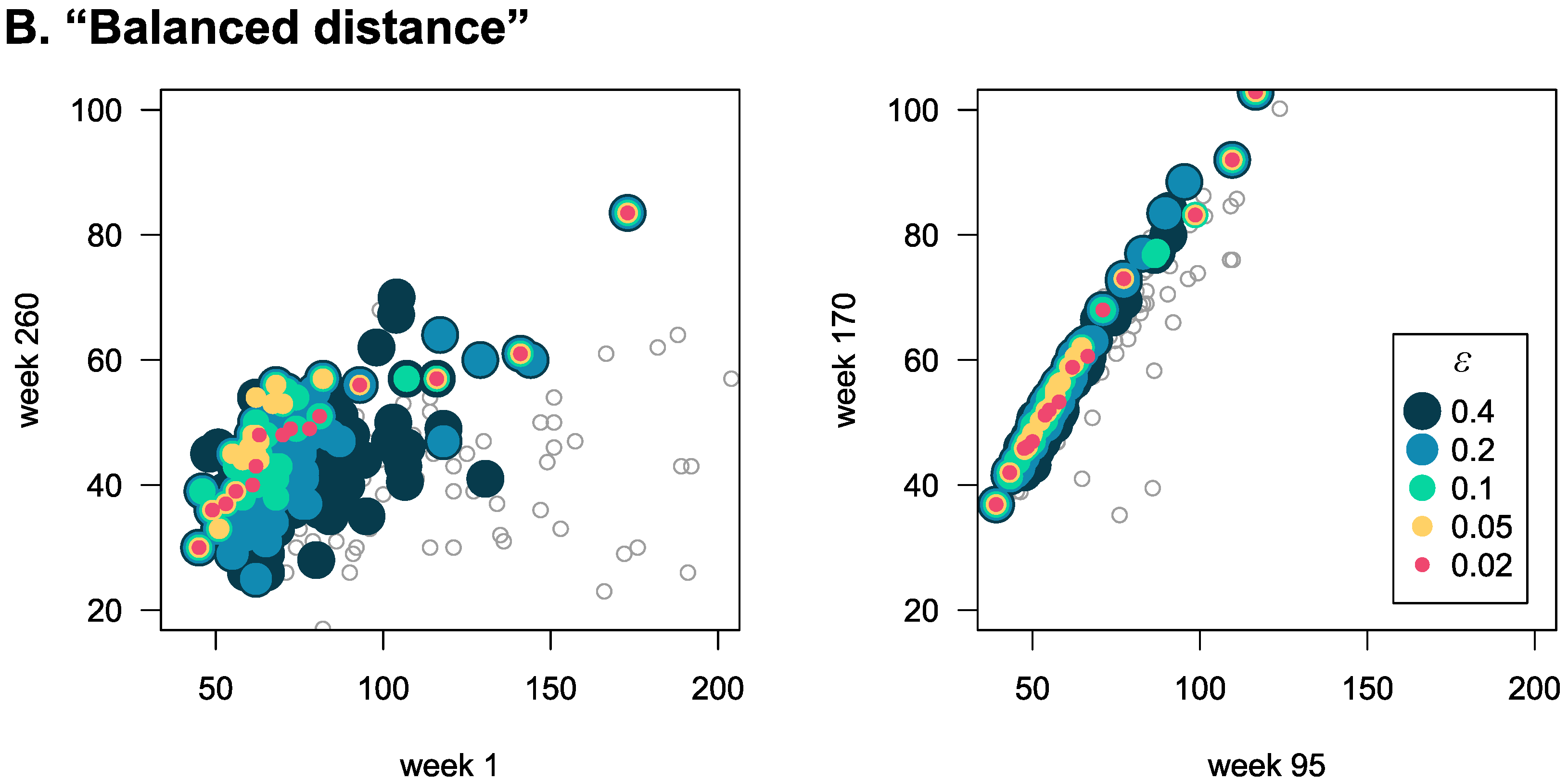
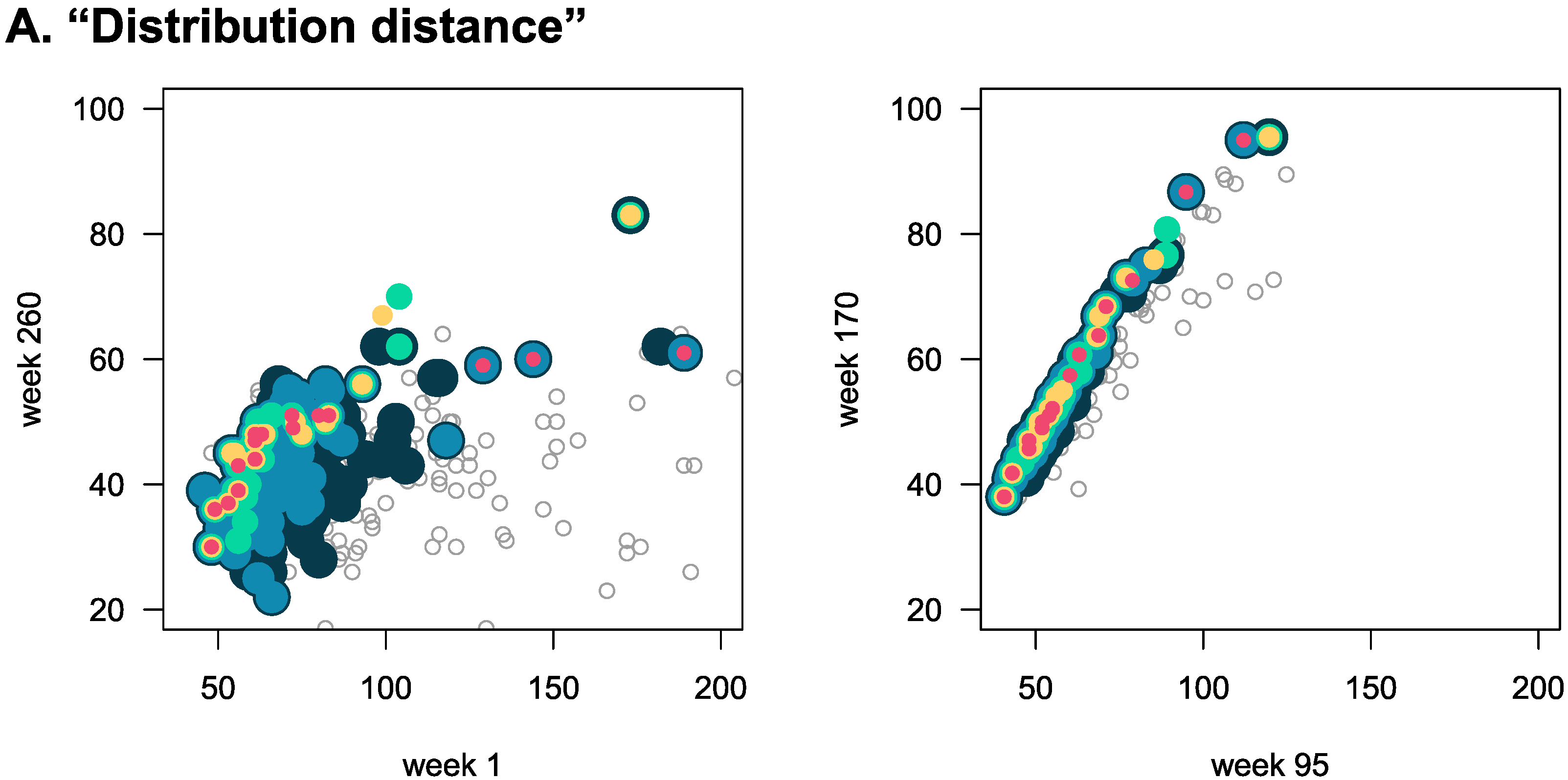
An alternative way to show the greatly reduced dimensionality of cliques is to plot the weekly average blood glucose values of patients along a few dimensions (Figure 3), both for patients that are not in cliques (grey empty circles), and those belonging to cliques (coloured full circles). We show this for both the “distribution” and “balanced” distances, and for both the first vs. last week (left panels), and between two randomly chosen weeks (right panels). We find that the smaller $\epsilon$ is, the more “in line” the data points of patients belonging to cliques are. Also, there is autocorrelation in the time series, and thus weeks closer to each other show smaller variation among the data points, both inside and outside of the clique.

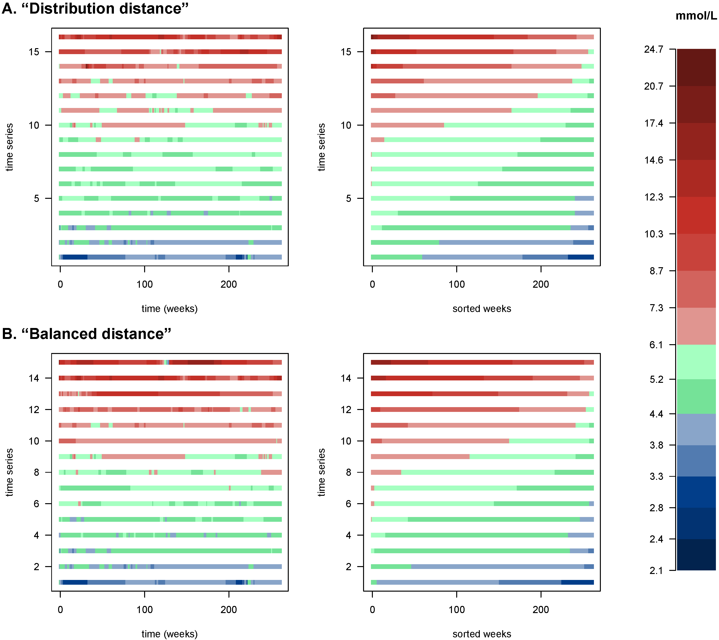
Finally, we show the original data for the patients in the $\epsilon =0.02$ cliques (Figure 4) in the order they appear on Figure 3, i.e., along the axis defined by those cliques. The left panels show the time series with their temporality preserved, emphasizing fluctuations; the right panels show the same series sorted by measured values, highlighting the blood glucose values’ distribution. Apparent in this figure is the fact that the cliques found identify meaningful gradients of the blood glucose dynamics of patients.

5. Summary

We proposed a procedure to locate approximately 1-dimensional linear manifolds based on the pair-wise distances between the objects of a given data set. The procedure requires the construction of an auxiliary graph and finding large cliques in this graph. At the first glance the auxiliary matrix looks overly large as the number of its nodes is $O\left(m^2\right)$, where m is the number of the objects of the original data set. We carried out numerical experiments to show that the procedure is computationally feasible in practice. The computations also confirmed that the proposed method is capable of locating approximately 1-dimensional linear manifolds in the data set.