Algorithms Utilized for Creep Analysis in Torque Transducers for Wind Turbines

Abstract

One of the fundamental challenges in analyzing wind turbine performance is the occurrence of torque creep under load and without load. This phenomenon significantly impacts the proper functioning of torque transducers, thus necessitating the utilization of appropriate measurement data analysis algorithms. In this regard, employing the least squares method appears to be a suitable approach. Linear regression can be employed to investigate the creep trend itself, while visualizing the creep in the form of a non-linear curve using a third-degree polynomial can provide further insights. Additionally, calculating deviations between the measurement data and the regression curves proves beneficial in accurately assessing the data.

1. Introduction

Wind energy has increased in popularity as a clean and sustainable source of electricity in recent years [1,2,3]. It is even more pronounced with the retreat from fossil fuels that is being amplified by ecological policies and strategies [4]. As new policies encourage the diversification of energy sources, this requires the development of new technologies and the intensification of research to improve existing ones. Energy acquired from wind has become a popular area of research, and wind turbines are a key element in power generation. It has become larger, more efficient, and more cost-effective, making wind power an increasingly important option for meeting energy needs [5,6].

Torque transducers are vital components in wind energy applications, facilitating the precise measurement and control of rotational forces within wind turbines. Sensitivity, range, accuracy, reliability, durability, and response time stand as key parameters for effective transducer selection. To assess the suitability of a torque transducer for dynamic or high-precision tasks, such as in the wind energy sector, its creep behavior must be known. This information can be used to optimize wind turbine performance by adjusting its operation based on changing wind conditions. Creep behavior refers to the gradual change in a material’s deformation over time when subjected to a constant load. For torque transducers, creep can affect their accuracy and performance. For this reason, the calibration of torque transducers corresponding to creep measurements must be carried out [7,8,9,10]. Studies have shown that the largest indications of the force transducer [11] and the torque transducer [12] in the first seconds of testing are most likely due to the mechanical properties of the materials from which the transducer is built.

Due to the elastic effect of the force transducer components (elastic material and strain gauges), there are slight changes in the output signal with constant force caused by creep. This effect is essential not only in long measurements, where the low creep value is very important, but also in short-term measurements. Creep error may be affected by, among others, the design of the force transducer and the elements of which it is built, the used force transducer electric cable, the measuring meter, the measurement axis, and the construction of the reference station itself.

Algorithms have emerged as powerful tools for analyzing and interpreting data obtained from torque transducers in wind energy applications. These algorithms enable the identification and quantification of creep, a phenomenon that can significantly impact the accuracy and reliability of torque measurements. By employing advanced algorithms, researchers can analyze the data collected from torque transducers to detect and correct for creep effects. These algorithms enable the estimation of true torque values by compensating for the creep-induced errors, thus enhancing the accuracy and reliability of torque measurements. One notable algorithm employed in creep study analysis is the Kalman filter. The Kalman filter, a recursive estimator, is widely employed in creep study analysis and has been successfully applied to analyze and compensate for creep effects in torque measurements from transducers used in wind energy applications [13]. Another algorithm that has shown promise in creep study analysis is the artificial neural network (ANN). ANNs are computational models that mimic biological neural networks and can accurately estimate true torque values in wind turbines by learning and recognizing complex patterns in the data and separating creep-induced errors [14,15,16].

Through the utilization of AI algorithms, researchers can create advanced models to analyze and forecast the effects of creep behavior on torque measurements, enhancing calibration and compensation techniques for improved accuracy and reliability in transducers employed in wind energy applications.

This work focuses on torque transducer creep testing. An approximation polynomial fit–straight line algorithm fits a set of points that are determined at regular intervals to a third-degree polynomial. Fit parameters and an averaged uncertainty corridor have been established.

2. Creep Study

2.1. Parameters Influencing Torque Transducer Creep

Various parameters, including temperature, applied load, calibration frequency, and environmental factors, influence the creep behavior of torque transducers [17,18,19,20].

• Temperature: Temperature variations significantly impact the performance and accuracy of torque transducers. High temperatures can lead to thermal expansion, causing materials to deform and introducing measurement errors. On the other hand, low temperatures can affect the viscosity of lubricants used within the transducers, resulting in changes in frictional forces and subsequently affecting their creep behavior.
• Applied Load: The magnitude and duration of the applied load directly influence the creep characteristics of torque transducers. High loads can cause deformation within the transducer’s sensing elements and alter their elastic properties, leading to an increased likelihood of creep. Moreover, long durations of sustained load can induce plastic deformation in the transducer, resulting in permanent changes in its calibration and accuracy.
• Calibration Frequency: Regular calibration is essential for maintaining the accuracy of torque transducers. The frequency at which these instruments are calibrated affects their creep behavior. Infrequent calibrations may lead to drift or systematic errors over time, impacting the reliability of torque measurements. Therefore, regular and timely calibration routines are necessary to ensure the optimal performance of torque transducers in wind energy applications.
• Environmental Factors: Environmental conditions, such as humidity and dust exposure, can influence the creep behavior of torque transducers. Moisture absorption may affect the transducer materials’ mechanical properties, leading to changes in creep rates. Additionally, dust or contaminants can accumulate on transducer surfaces, altering their friction characteristics and introducing measurement errors. Therefore, protection measures to mitigate these environmental factors are essential for maintaining accurate torque measurements.

Understanding the key parameters influencing torque transducer creep is essential for ensuring accurate and reliable measurements in wind energy applications.

2.2. Experimental Conditions

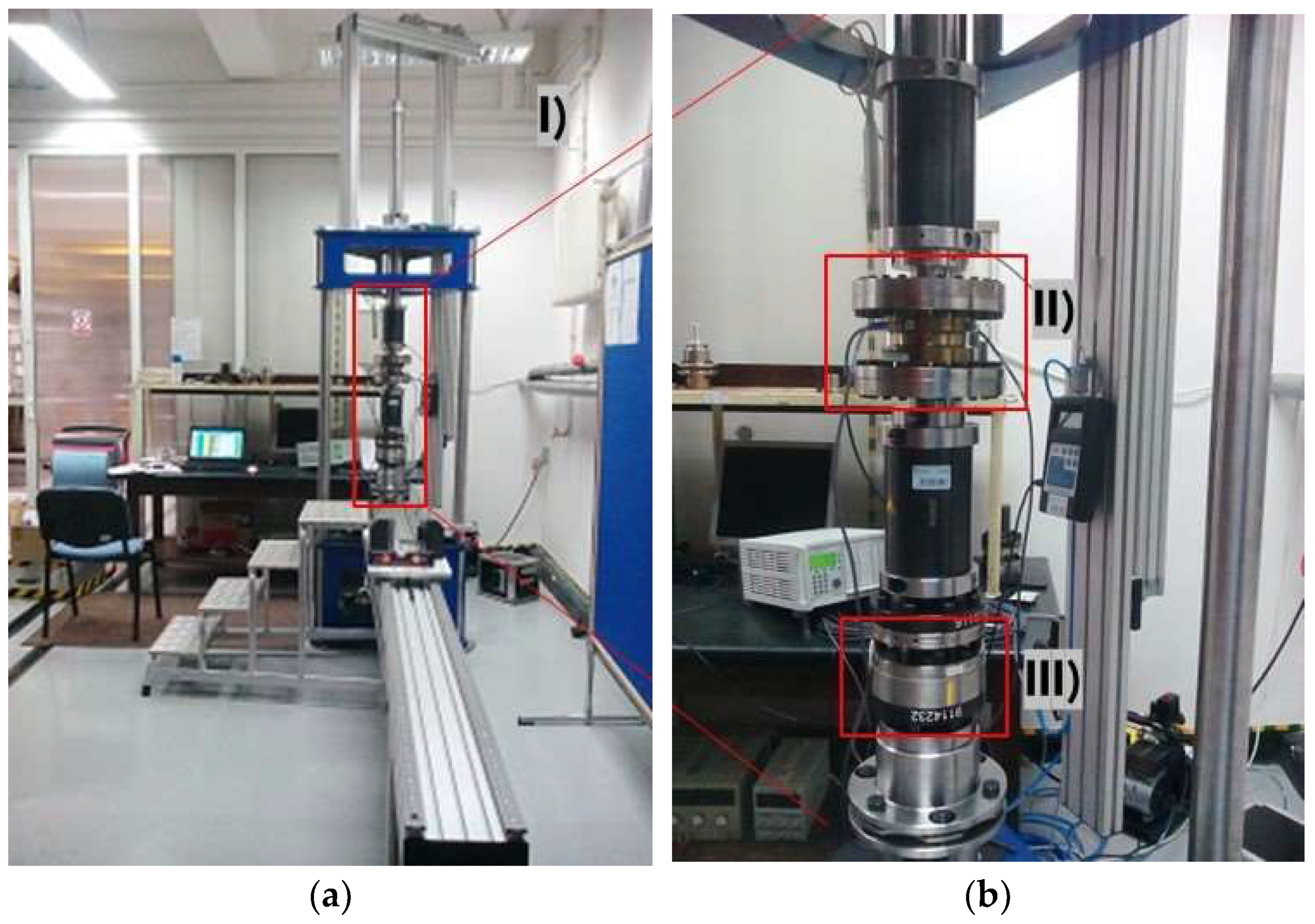
The torque standard machine (TSM) at the Central Office of Measures (GUM) in Poland is a reference machine which uses a DC motor to apply torque and a calibrated reference torque transducer to measure torque (see Figure 1). This TSM is able to generate clockwise and anti-clockwise torque in a range from 10 N·m up to 5 kN·m with an expanded relative uncertainty 0.04% (k = 2). As a reference transducer, the HBK transducer (Hottinger Bruel and Kjear) working in the range from 200 N·m to 5000 N·m (type TB2/3000 N m; #181030110) was used in GUM’s TSM. The amplifier used was a MGCplus/ML38B/DMP41 (with a 0.5 Hz Bessel filter), characterized by the best accuracy class and a resolution of 1 ppm in the measuring interval ±2.5 mV/V. The creep tests were conducted at ambient temperatures for the 2 kN·m torque transducer in clockwise and anti-clockwise directions following the ISO 376:2011 standard.

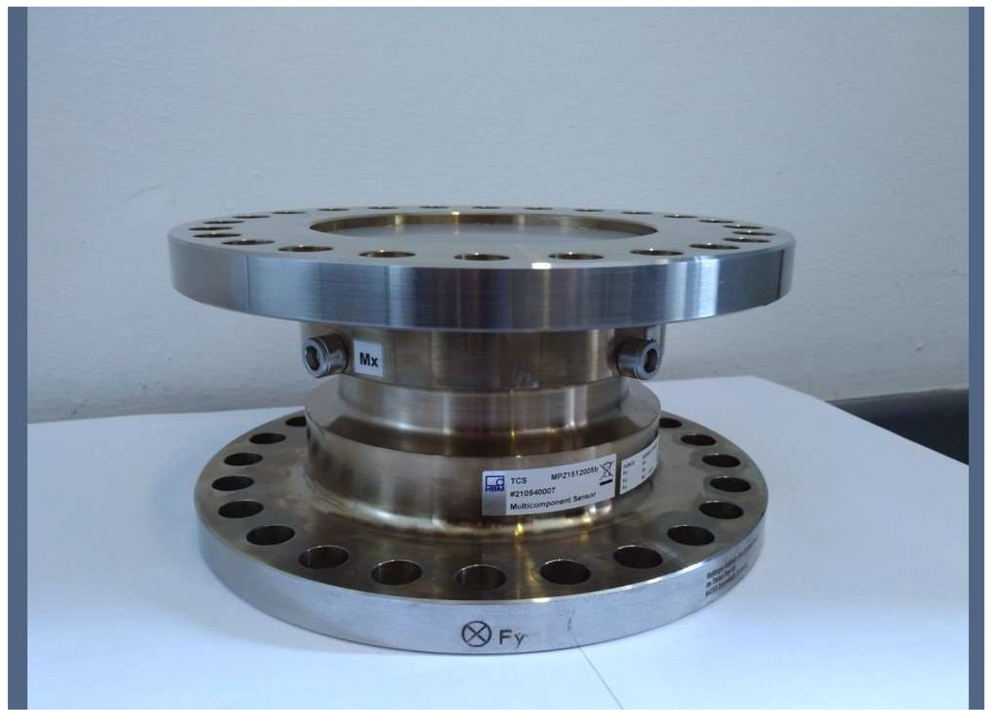
This HBK 2 kN·m multicomponent torque transducer (type MPZ1512005b, serial no. #210940007), intended to measure torque in both clockwise and anti-clockwise directions, is presented in Figure 2. What is important about this torque transducer is not only its mechanical resemblance to the 5 MN·m torque transducer but also its additional bridges to measure axial force F_z and bending moments M_x and M_y.

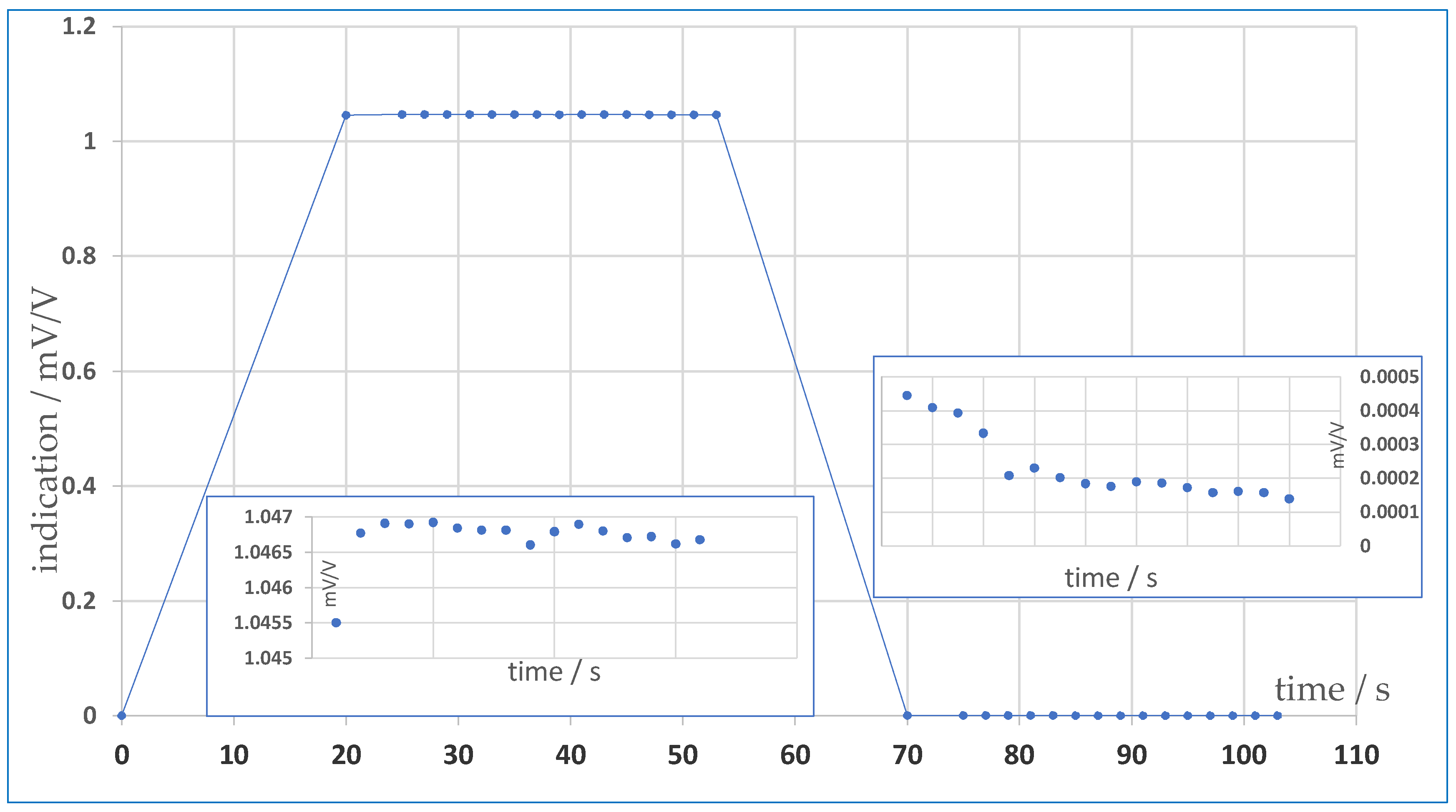
The creep study was conducted for eight measurement points ranging from 200 N·m to 2000 N·m. A measured signal was observed in each point by 33 s from the 20th second after loading. Additionally, at each measurement point, the signal behavior was tested without loading in the same time interval, starting at the 70th second. The torque transducer indication is given in electrical units (mV/V). A total of 16 readings represent the creep at each measurement point (Figure 3 and

Table 1. Measured signal values from the transmitter for two measurement levels.

High Level of Torque		Low Level of Torque
Time t (s)	Signal y (mV/V)	Time t (s)	Signal y (mV/V)
20	1.045500	70	0.000445
25	1.046769	75	0.000409
27	1.046910	77	0.000393
29	1.046901	79	0.000333
31	1.046923	81	0.000208
33	1.046842	83	0.000230
35	1.046813	85	0.000202
37	1.046813	87	0.000184
39	1.046604	89	0.000176
41	1.046791	91	0.000190
43	1.046897	93	0.000186
45	1.046798	95	0.000172
47	1.046705	97	0.000158
49	1.046722	99	0.000161
51	1.046618	101	0.000158
53	1.046679	103	0.000139

). The dependence of the measured points of the electrical signal y_i at intervals t_i both for the statically determined torque of force and its lack-zero forcing of the torque, in general, is not reproducible and depends on many reasons related to the torque standard machine and environmental conditions. It is seen as a stochastic process. From the point of view of determining the characteristics of the transducer, the most important are the average values in the time-determined signal (the value of the measurand) and the average value of signal uncertainty (the minimum width of the coverage interval in which the true value of the signal is included).

Therefore, the creep analysis is based on the least squares method with the use of polynomial and linear regression, whereby, in general, the nonlinear function is adjusted to the individual measuring points.

For this purpose, both a linear function with two parameters, which represent the direction of the creep at each measurement point, and a third-degree polynomial function with three and four parameters were used. Third-degree polynomial functions, thanks to having saddle points, take into account the nonlinear effects of the time dependence of the signal. For measurement points under load, in most cases it is an increasing trend, but for measurement points without load, no clear trend can be distinguished. Further analysis of the line of best fit in the figure indicates that the scatter of the data about the line is not random but exhibits a definite trend.

In order to adjust the parameters of a given nonlinear function, the measured values of the points and their estimated uncertainties are necessary. The combined standard uncertainty associated with a single measuring point is determined using eight contributions by the equation:

$$u_{\mathrm{T}\mathrm{S}\mathrm{M}}^2=\sum _{i=1}^8{u}_i^2$$

(1)

where:

u₁—standard uncertainty of calibration results of reference transducers when cubic fitting functions are used;

u₂—standard uncertainty due to short-term creep of reference transducers;

u₃—standard uncertainty associated with the long-term drift of reference transducers;

u₄—standard uncertainty due to misalignment of the device under calibration;

u₅—standard uncertainty associated with the resolution and stability of the indicating device (amplifier);

u₆—standard uncertainty associated with using reference transducers in partial ranges;

u₇—standard uncertainty due to stability of torque transmission on shafts;

u₈—standard uncertainty due to the influence of the variation in temperature on reference transducers.

In addition, a single measurement point at a given moment of time in general is determined by a total of 13 uncorrelated corrections, 8 of which are directly related to the standard measurement uncertainty of the torque generation.

The measurement points in a successive moments of time do not indicate the same value of the signal from the transducer. The final values of the signal after the equilibrium state has been established do not represent the measured value either. It is a time relationship $y=f\left(t\right)$ that reflects a measurement that is entirely a stochastic process, and therefore the use of standard methods will be insufficient to determine the average value of the measured level. For example, to determine the uncertainty value of the time-dependent signal measurement, the deviation is often called Allan’s deviation, or square root of Allan’s variance, which is not used in stationary systems where the time dependence is no longer important. In this case, the assumption about the stationarity of the signal measurement process is doomed to be unreliable.

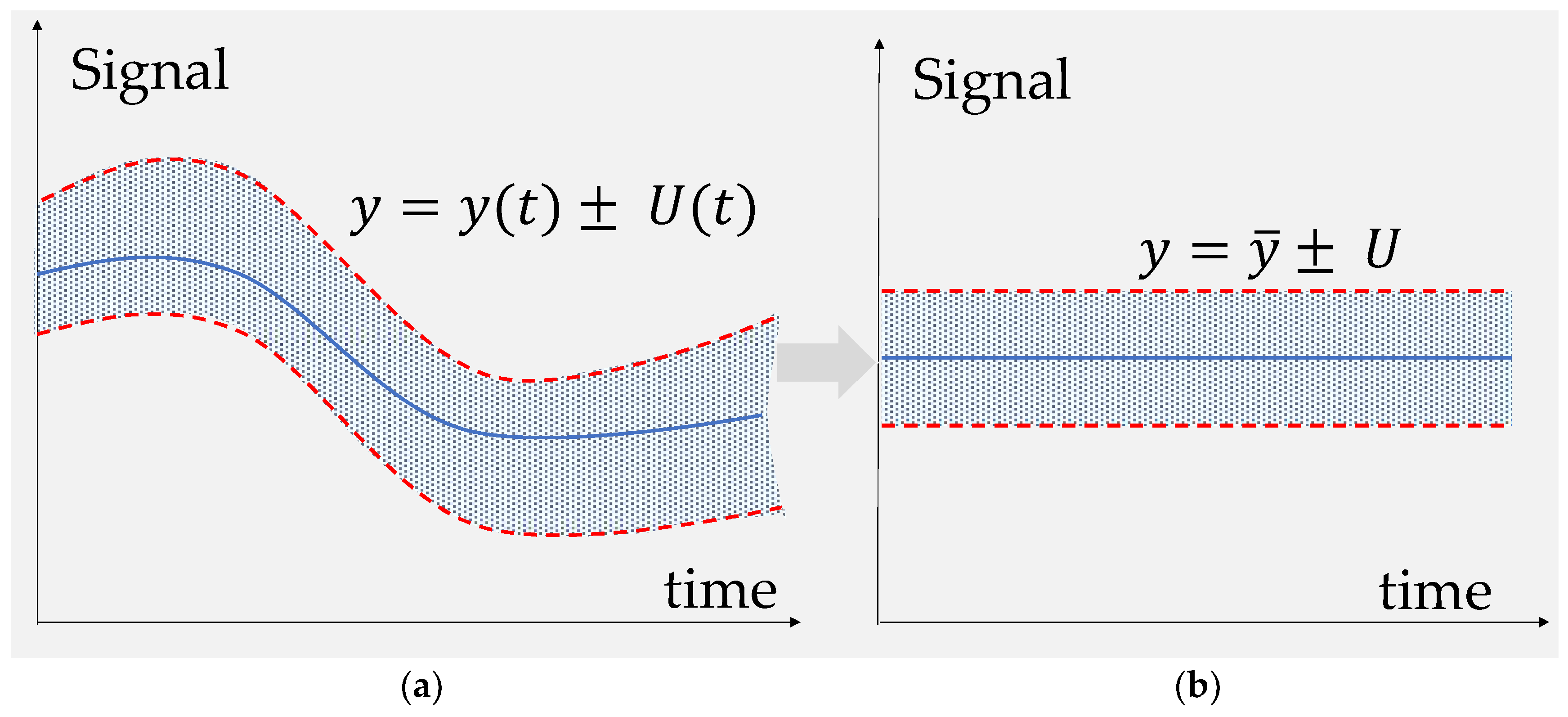
In order to determine the characteristics of the torque converter, it is necessary to determine the average signal level y from the transducer measured at preset intervals. This signal is subject to so-called creep, changing its value at each sampled moment of time. In Figure 4a, a sample relationship of the signal as a function of time is presented, y(t), including the expanded uncertainty of the coverage corridor, which is also a function of time in general, U(t). However, in order to determine the characteristics, it is necessary to determine the average value of the signal $\overline{y}$ and the constant width of the signal uncertainty corridor U, which do not change at any given torque measurement points (Figure 4b).

3. Least Square Method

The basic tool used to fit a nonlinear relationship to measurement points is the least squares method. In the general approach, it is the WTLS (weighted total least square) method [21,22,23,24,25,26,27] that takes into account all the generally differing uncertainties of the coordinates of the points and the various correlations between the coordinates of the measurement points. So, the problem is to determine the global minimum of the criteria function [28,29]:

$${\varphi }_{ty}=\left[\mathsf{\Delta }\mathit{t},\mathsf{\Delta }\mathit{Y}\right]{\mathit{U}}^{-1}\left[\begin{array}{c}\mathsf{\Delta }\mathit{t}\\ \mathsf{\Delta }\mathit{Y}\end{array}\right]\to min$$

(2)

of residua vector time and signal and covariance matrix $\mathit{U}$ with dependence of nonlinear function y = f(t) with respect to which the time deviations of the signal from the converter are calculated.

4. The Proposed Model

The linear or nonlinear functions of time are described by the polynomial expansion of a Taylor series y = f(t, c) = c₀ + c₁t + c₂t² + … + c_mt^m and the match parameter vector c = [c₀, c₁, c₂, …, c_m]^T. This means that in order to determine the fit vector, the following are generally required: m-nonlinear equations [30,31,32,33,34,35,36,37]. This expansion also represents the application of many complex elementary functions describing a given physical process. In our case, it is a process stretched over time of “creeping” a physical quantity to be measured, in this case the moment of force, resulting, inter alia, from the inertia of the processes occurring during the measurement on the measuring standard.

The basic tool used to fit a nonlinear relationship to measurement points is the least squares method. In the general approach, it is the WTLS method that takes into account all the generally different uncertainties of the coordinates of the points and the various correlations between the coordinates of the measurement points.

The parameters of this schematic view are determined from the vector equation for the least squares method, taking into account not only the coordinates of the measured measurement points but also the uncertainty of the signal and time, as well as all possible correlations between them related to environmental conditions and the properties of the measuring system.

The general optimization condition boils down to maximizing the greatest likelihood function, which means minimizing the dimensionless criterion function with the most general equation for the least squares method (WTLS):

$${\varphi }_{ty}\left(\mathsf{\Delta }\mathit{t},\mathsf{\Delta }\mathit{Y}\right)=\left[\mathsf{\Delta }\mathit{t},\mathsf{\Delta }\mathit{Y}\right]{{\mathit{U}}_{\mathit{T}\mathit{S}}}^{-1}\left[\begin{array}{c}\mathsf{\Delta }\mathit{t}\\ \mathsf{\Delta }\mathit{Y}\end{array}\right]=\left[\mathsf{\Delta }\mathit{t},\mathsf{\Delta }\mathit{Y}\right]{\left[\begin{array}{cc}{\mathit{U}}_{\mathit{t}}& {\mathit{U}}_{\mathit{t}\mathit{Y}}\\ {\mathit{U}}_{\mathit{t}\mathit{Y}}^{\mathit{T}}& {\mathit{U}}_{\mathit{Y}}\end{array}\right]}^{-1}\left[\begin{array}{c}\mathsf{\Delta }\mathit{t}\\ \mathsf{\Delta }\mathit{Y}\end{array}\right]\to min$$

(3)

where U_t, U_Y, U_tY are covariance matrixes that are single parts of the covariance matrix ${\mathit{U}}_{\mathit{T}\mathit{S}}=\left[\begin{array}{cc}{\mathit{U}}_{\mathit{t}}& {\mathit{U}}_{\mathit{t}\mathit{Y}}\\ {\mathit{U}}_{\mathit{t}\mathit{Y}}^{\mathit{T}}& {\mathit{U}}_{\mathit{Y}}\end{array}\right]$ appropriate for the time variable t and the measured signal y in n-points taking into account autocorrelations and a covariance matrix taking into account the effects of cross correlation between time and signal coordinates, while Δt, ΔY denote vectors containing deviation values for time Δt₁, …, Δt_n and for the signal Δy₁ = f(t₁ + Δt₁, c) − f(t₁, c), …, Δy_n = f(t_n + Δt_n, c) − f(t_n, c) at subsequent measuring points t₁,…, t_n. In the special case of no correlation, the dependence of the minimum criterion function (3) means a minimum of:

$${\varphi }_{ty}\left(\mathsf{\Delta }\mathit{t},\mathsf{\Delta }\mathit{Y}\right)=\sum _{i=1}^n\frac{{\Delta t_i}^2}{u^2\left(t_i\right)}+\frac{{{\Delta y}_i}^2}{u^2\left(y_i\right)}\to min$$

(4)

where u²(t_i) and u²(y_i) are variances (squared uncertainties) for time deviations Δt_i and for signal deviations Δy_i. The most commonly used method of least squares is the OLSs (ordinary least squares) or special case of TLSs (total least squares for identical values of uncertainties of time and signal) without taking into account the uncertainty of the abscissa variable in this case of time u(t) = 0, assuming that all signal uncertainties are the same u²(y_i) = const.

In a specific case, i.e., where u²(t_i) → 0 and values t_i are measured exactly, condition (4) reduces to the form of:

$${\varphi }_y\left(\mathsf{\Delta }\mathit{Y}\right)=\sum _{i=1}^n\frac{{{\Delta y}_i}^2}{u^2\left(y_i\right)}\to min$$

(5)

As long as condition (5) leads to analytical solutions for any nonlinear function represented in the Taylor series (also for constant uncertainties (5)), using the determinant method, finding the minimization condition included in Equation (4) or the most general Equation (3) requires the use of numerical methods.

However, there is an approximate method, which will be presented in the following section, based on the algorithm for numerical straight line fitting solutions. This algorithm will make it possible to fit a nonlinear function given in the form of two polynomial functions of tertiary degree in the form described by y = a₃t³ + a₂t² + a₁t + a₀ and y = b₂t³ + b₁t + b₀, and a linear function y = at + b constituting a trend line for the above relationships. Parameters a_k (k = 0, 1, 2, 3), b_l (l = 0, 1, 2), and a and b will be determined by the proposed method using an appropriate numerical algorithm.

5. Analytical Solutions

For the weighted least squares method (WLS), the optimization equation for minimizing squared distances in the direction of OY for the set of n-measurement points with coordinates (t_i, y_i) and leads as a result of zeroing the first partial derivatives after the slope parameter a and intercept b for a straight line and parameters a_i and b_i for tertiary curves for analytical solutions has the form below.

5.1. For Linear Curve (y = ax + b)

$$a=\frac{S{S}_{ty}-S_t{S}_y}{{SS}_{tt}-{{(S}_t)}^2},$$

(6a)

$$b=\frac{S_y{S}_{tt}-S_t{S}_{ty}}{S{S}_{tt}-{{(S}_t)}^2},$$

(6b)

where auxiliary parameters $S,$ $S_t, S_{tt}, S_y, S_{ty}$ are defined by:

$$S=\sum _{i=1}^n\frac{1}{u^2\left(y_i\right)},$$

(7a)

$$S_t=\sum _{i=1}^n\frac{t_i}{u^2\left(y_i\right)},$$

(7b)

$$S_{tt}=\sum _{i=1}^n\frac{t_i^2}{u^2\left(y_i\right)},$$

(7c)

$$S_y=\sum _{i=1}^n\frac{y_{i,}}{u^2\left(y_i\right)},$$

(7d)

$$S_{ty}=\sum _{i=1}^n\frac{t_i{y}_i}{u^2\left(y_i\right)}.$$

(7e)

5.2. For Polynomial of Third Order (y = b₂t³ + b₁t + b₀)—Type I

First derivatives for the parameters b_j, where j = 0, 1, 3

$$\sum _{i=1}^n(y_i-b_3{t}_i^3-b_1{t}_i-b_0)\frac{t_i^j}{u^2\left(y_i\right)}=0$$

(8)

a system of three linear equations solvable by the determinant method is obtained:

$$\left[\begin{array}{c}\begin{array}{c}{b}_3\end{array}\\ \begin{array}{c}{b}_1\\ b_0\end{array}\end{array}\right]={\left[\begin{array}{cc}\begin{array}{c}{R}_t^6\end{array}& \begin{array}{cc}{R}_t^4& R_t^3\end{array}\\ \begin{array}{c}{R}_t^4\\ R_t^3\end{array}& \begin{array}{cc}{R}_t^2& R_t^1\\ R_t^1& R_t^0\end{array}\end{array}\right]}^{-1}\left[\begin{array}{c}\begin{array}{c}{R}_{ty}^3\end{array}\\ \begin{array}{c}{R}_{ty}^1\\ R_{ty}^0\end{array}\end{array}\right]$$

(9)

where notation used:

$$R_t^j=\sum _{i=1}^n\frac{t_i^j}{u^2\left(y_i\right)},$$

(10a)

$$R_{ty}^j=\sum _{i=1}^n\frac{y_i{t}_i^j}{u^2\left(y_i\right)}, j=0, 1, 3.$$

(10b)

5.3. For Polynomial of Third Order (y = a₃t³ + a₂t² + a₁t + a₀)—Type II

First derivatives for the parameters a_j, where j = 0, 1, 2, 3

$$\sum _{i=1}^n(y_i-a_3{t}_i^3-a_2{t}_i^2-a_1{t}_i-a_0)\frac{t_i^j}{u^2\left(y_i\right)}=0,$$

(11)

a system of four linear equations solvable by the determinant method is obtained:

$$\left[\begin{array}{c}\begin{array}{c}{a}_3\\ a_2\end{array}\\ \begin{array}{c}{a}_1\\ a_0\end{array}\end{array}\right]={\left[\begin{array}{cc}\begin{array}{cc}{S}_t^6& S_t^5\\ S_t^5& S_t^4\end{array}& \begin{array}{cc}{S}_t^4& S_t^3\\ S_t^3& S_t^2\end{array}\\ \begin{array}{cc}{S}_t^4& S_t^3\\ S_t^3& S_t^2\end{array}& \begin{array}{cc}{S}_t^2& S_t^1\\ S_t^1& S_t^0\end{array}\end{array}\right]}^{-1} \left[\begin{array}{c}\begin{array}{c}{S}_{ty}^3\\ S_{ty}^2\end{array}\\ \begin{array}{c}{S}_{ty}^1\\ S_{ty}^0\end{array}\end{array}\right]$$

(12)

and below notation is used:

$$S_t^j=\sum _{i=1}^n\frac{t_i^j}{u^2\left(y_i\right)},$$

(13a)

$$S_{ty}^j=\sum _{i=1}^n\frac{y_i{t}_i^j}{u^2\left(y_i\right)}, j=0, 1, 3.$$

(13b)

The last function, type II, describes more complicated relationships for a given set of measurement points than type I, although type I and type II are equivalent if you make a corresponding shift on the timeline.

6. Approximate WTLS Solutions for Nonlinear Functions

It turns out that in the case of the occurrence of generally different uncertainties for the time variable t_i and the measured signal y_i and correlations described by the covariance matrix, ${\mathit{U}}_{\mathit{T}\mathit{S}}$ nonlinear relationship y = f(t) can be represented in the form of a linear relationship y = θ₁ξ(t, β) + θ₀, where the function ξ(t, β) is a transforming function, and θ₁, θ₀ and, in general, the vector β are the parameters of the fitting function, which result from the fitting of the function and the minimization of the criterion function, which approximately transforms to the form [29]:

$$\begin{gathered} {\varphi }_{ty}\left(\mathsf{\Delta }\mathit{t},\mathsf{\Delta }\mathit{Y}\right)=\left[\mathsf{\Delta }\mathit{t},\mathsf{\Delta }\mathit{Y}\right]\mathit{L}{\mathit{L}}^{-1}{\left[\begin{array}{cc}{\mathit{U}}_{\mathit{t}}& {\mathit{U}}_{\mathit{t}\mathit{Y}}\\ {\mathit{U}}_{\mathit{t}\mathit{Y}}^{\mathit{T}}& {\mathit{U}}_{\mathit{Y}}\end{array}\right]}^{-1}{\mathit{L}}^{-1}\mathit{L}\left[\begin{array}{c}\mathsf{\Delta }\mathit{t}\\ \mathsf{\Delta }\mathit{Y}\end{array}\right] \\ \approx \left[\mathsf{\Delta }\mathit{\xi },\mathsf{\Delta }\mathit{Y}\right]{\left[\begin{array}{cc}{\mathit{U}}_{\mathit{\xi }}& {\mathit{U}}_{\mathit{\xi }\mathit{Y}}\\ {\mathit{U}}_{\mathit{\xi }\mathbf{Y}}^{\mathit{T}}& {\mathit{U}}_{\mathit{Y}}\end{array}\right]}^{-1}\left[\begin{array}{c}\mathsf{\Delta }\mathit{\xi }\\ \mathsf{\Delta }\mathit{Y}\end{array}\right]={\varphi }_{\xi y}\left(\mathsf{\Delta }\mathit{\xi },\mathsf{\Delta }\mathit{Y},\mathit{\beta }\right) \end{gathered}$$

(14)

and diagonal matrix L size of 2n × 2n shall be determined by the first n elements as derivatives of functions ξ′(t_i,  β) at subsequent measurement points, and the following n, an identical diagonal value, is equal to a value of one. The laws of error and uncertainty propagation have been used by multiplying the first derivative of the transforming function, respectively, by error of time and uncertainty of time:

$$\Delta \xi \approx {\xi }^{\prime }\left(t,\mathit{\beta }\right)\Delta t,$$

(15a)

$$u\left(\xi \right)\approx \left|{\xi }^{\prime }\left(t,\mathit{\beta }\right)\right|u\left(t\right)$$

(15b)

It follows that dependencies ϕ_ξy(θ₁) and ϕ_ξy(θ₀) for the selected parameter vector $\mathit{\beta }=\left[{\beta }_1,{\beta }_2\right]$ are quasi-square and described by [22]:

$${\varphi }_{\xi y}\left({\theta }_1\right)={{\theta }_1}^2\left(P_{\mathit{t}\mathit{t}}-\frac{P_t^2}{P}\right)+2\left(\frac{P_{\mathit{t}}{P}_{\mathit{y}}}{P}-P_{\mathit{t}\mathit{y}}\right){\theta }_1+P_{\mathit{y}\mathit{y}}-\frac{P_y^2}{S}$$

(16)

where

$$P={\mathbf{1}}^{\mathit{T}}{\mathit{U}}_{\mathit{Y}\mathit{e}\mathit{f}\mathit{f}}^{-\mathbf{1}}\mathbf{1},$$

(17a)

$$P_t={{\mathit{\xi }}^{\mathit{T}}{\mathit{U}}_{\mathit{Y}\mathit{e}\mathit{f}\mathit{f}}^{-\mathbf{1}}\mathbf{1}=\mathbf{1}}^{\mathit{T}}{\mathit{U}}_{\mathit{Y}\mathit{e}\mathit{f}\mathit{f}}^{-\mathbf{1}}\mathit{\xi },$$

(17b)

$$P_y={\mathit{Y}}^{\mathit{T}}{\mathit{U}}_{\mathit{Y}\mathit{e}\mathit{f}\mathit{f}}^{-\mathbf{1}}\mathbf{1}={\mathbf{1}}^{\mathit{T}}{\mathit{U}}_{\mathit{Y}\mathit{e}\mathit{f}\mathit{f}}^{-\mathbf{1}}\mathit{Y},$$

(17c)

$$P_{tt}={\mathit{\xi }}^{\mathit{T}}{\mathit{U}}_{\mathit{Y}\mathit{e}\mathit{f}\mathit{f}}^{-\mathbf{1}}\mathit{\xi },$$

(17d)

$$P_{ty}={\mathit{\xi }}^{\mathit{T}}{\mathit{U}}_{\mathit{Y}\mathit{e}\mathit{f}\mathit{f}}^{-\mathbf{1}}\mathit{Y}={\mathit{Y}}^{\mathit{T}}{\mathit{U}}_{\mathit{Y}\mathit{e}\mathit{f}\mathit{f}}^{-\mathbf{1}}\mathit{\xi },$$

(17e)

$$P_{yy}={\mathit{Y}}^{\mathit{T}}{\mathit{U}}_{\mathit{Y}\mathit{e}\mathit{f}\mathit{f}}^{-\mathbf{1}}\mathit{Y}$$

(17f)

and effective inverse covariance matrix is given by:

$${\mathit{U}}_{\mathit{Y}\mathit{e}\mathit{f}\mathit{f}}^{-\mathbf{1}}={\mathit{U}}_{\mathbf{22}}-\left({\mathit{U}}_{\mathbf{12}}^{\mathit{T}}+{\theta }_{\mathbf{1}}{\mathit{U}}_{\mathbf{22}}\right){\mathit{V}}^{-\mathbf{1}}\left({\mathit{U}}_{\mathbf{12}}+{\theta }_{\mathbf{1}}{\mathit{U}}_{\mathbf{22}}\right)$$

(18)

and $\mathit{V}={\mathit{U}}_{\mathbf{11}}+{\theta }_{\mathbf{1}}\left({\mathit{U}}_{\mathbf{12}}^{\mathit{T}}+{\mathit{U}}_{\mathbf{12}}\right)+{{\theta }_{\mathbf{1}}}^{\mathbf{2}}{\mathit{U}}_{\mathbf{22}}$ and matrixes ${{\mathit{U}}_{\mathbf{11}},\mathit{U}}_{\mathbf{12}},{\mathit{U}}_{\mathbf{22}}$ are the corresponding parts of the inverse covariance matrix ${\mathit{U}}_{\mathit{T}\mathit{S}}^{-\mathbf{1}}={\left[\begin{array}{cc}{\mathit{U}}_{\mathit{\xi }}& {\mathit{U}}_{\mathit{\xi }\mathit{Y}}\\ {\mathit{U}}_{\mathit{\xi }\mathit{Y}}^{\mathit{T}}& {\mathit{U}}_{\mathit{Y}}\end{array}\right]}^{-\mathbf{1}}$ = $\left[\begin{array}{cc}{\mathit{U}}_{\mathbf{11}}& {\mathit{U}}_{\mathbf{12}}\\ {\mathit{U}}_{\mathbf{12}}^{\mathit{T}}& {\mathit{U}}_{\mathbf{22}}\end{array}\right]$ and are functions of only one parameter ${\theta }_1$ or ${\theta }_0={(P}_y-{\theta }_1{P}_t)/P$, and these functions have quasi vertices [28]. By determining for a series of points within the accepted test interval ${\theta }_{1L}$ < ${\theta }_{1H}$ for selected values of vector parameters $\mathit{\beta }$ values of the local minimum and then looking for the value of the vector $\mathit{\beta }$ (the easiest one-dimensional vector), it is possible to minimize the criterion function by obtaining a global minimum at the points: ${\theta }_{1min}$, ${\mathit{\beta }}_{min}$.

Algorithm Schema for the Method WTLS

The algorithm is implemented in four steps:

(1)

For a given fitting function, e.g., y = a₃t³ + a²t² + a₁t + a₀, we create a function ξ(t, β), in this case, ξ(t, [β₁, β₂]) = t³ + β₁t² + β₂t, where β₁ = a₂/a₃ and β₂ = a₁/a₃ by setting initial values β₁ and β₂, which we calculate numerically with fixed steps h_β1 i h_β2 so that these values are in the ranges of β_1L ≤ β₁ ≤ β_1H and β_2L ≤ β₂ ≤ β_2H;

(2)

Then, on the basis of the given covariance matrix ${\mathit{U}}_{\mathit{T}\mathit{S}}$, we determine the matrix product L ${\mathit{U}}_{\mathit{T}\mathit{S}}$L, where n first diagonal elements of a matrix L are defined by ξ′(t_i, β) = 3t_i² + 2β₁t_i + β₂;

(3)

At the end, we designate a series of points θ_1j and specify the values of the θ₁ with a step h_θ1 from the selected range θ_1L ≤ θ_1j ≤ θ_1H (j = 1, …, M) = [(θ_1H − θ_1L)/h_θ1] and calculate characteristics ϕ_ξy(θ₁) and the resulting characteristics of the ϕ_ξy(θ₀), whereby the points θ_1j should be selected in such a way that they make visible a quasi-minimum (quasi vertex);

(4)

Repeat the above points one by one, first adjusting the β₁, and next β₂ or vice versa, until the global minimum of the criterion function is obtained ϕ_yξmin for fitting parameters a₃ = θ_1min, a₂ = θ_1min β_1min, a₁ = θ_1min β_2min and a₀ = θ_0min.

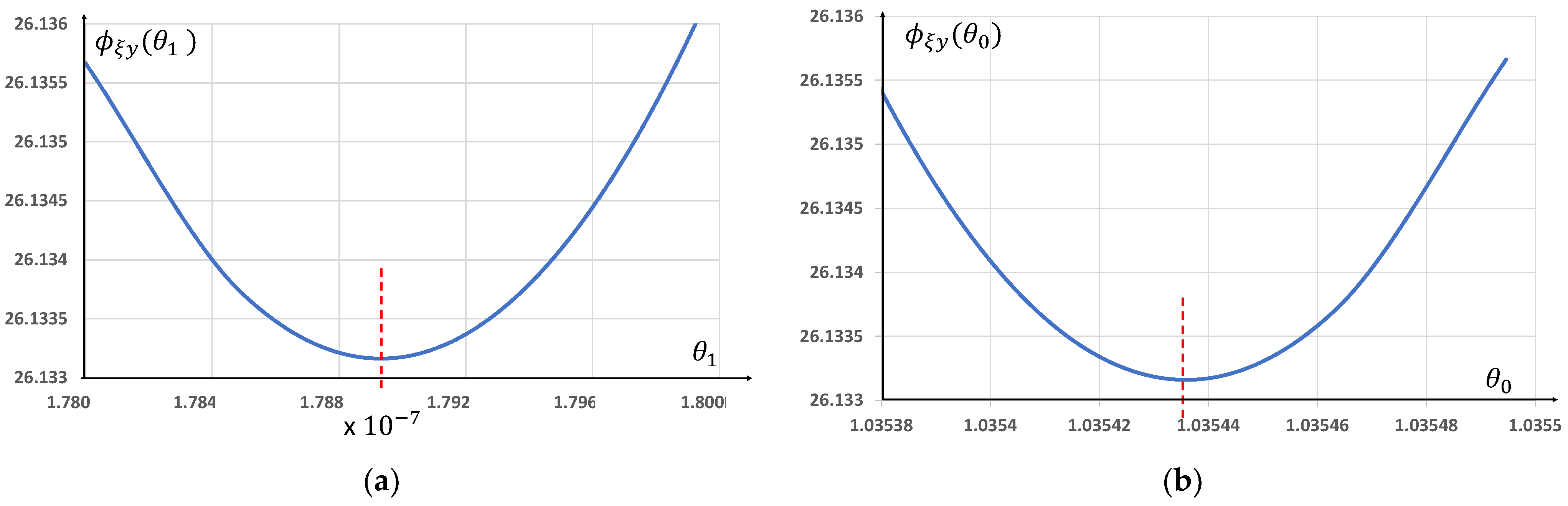
In the case of a simplified third-degree fitting function y = b₃t³ + b₁t + b₀ function ξ(t, β₁) = t³ + β₁t and then the values of the adjusted parameters due to the presence of only one parameter β₁ shall be, respectively, calculated from b₃ = θ_1min, b₁ = θ_1min β_1min and b₀ = θ_0min. Exemplary characteristics ϕ_ξy(θ₁) and ϕ_ξy(θ₀) are below in Figure 5.

7. Straight Line Fit Results (Trend Line)

A straight line adjustment y = ax + b is implemented, taking into account only constant uncertainty values. In the first approach in Equation (5), signal uncertainty constants have been assumed to be u(y_i) = 0.0001 mV/V, and analytical solutions have been used (6, 7). In the second approach, an approximate solution for Equation (4) has been used with constant uncertainties u(t_i) = 0.3 s, u(y_i) = 0.0001 mV/V using the algorithm of method WTLS for straight line, which is described in Section 5.1.

The following time dependencies were obtained for matching using the same method as OLSs—the first case:

• For adjustments of the low level of signal: y = −9.0 × 10⁻⁶ t + 0.001024 with the value of the criterion function ϕ_ytmin = 3.36;
• For adjustments high level of signal: y = 1.006 27 × 10⁻⁵ t + 1.046325 with the value of the criterion function ϕ_ytmin = 141.78.

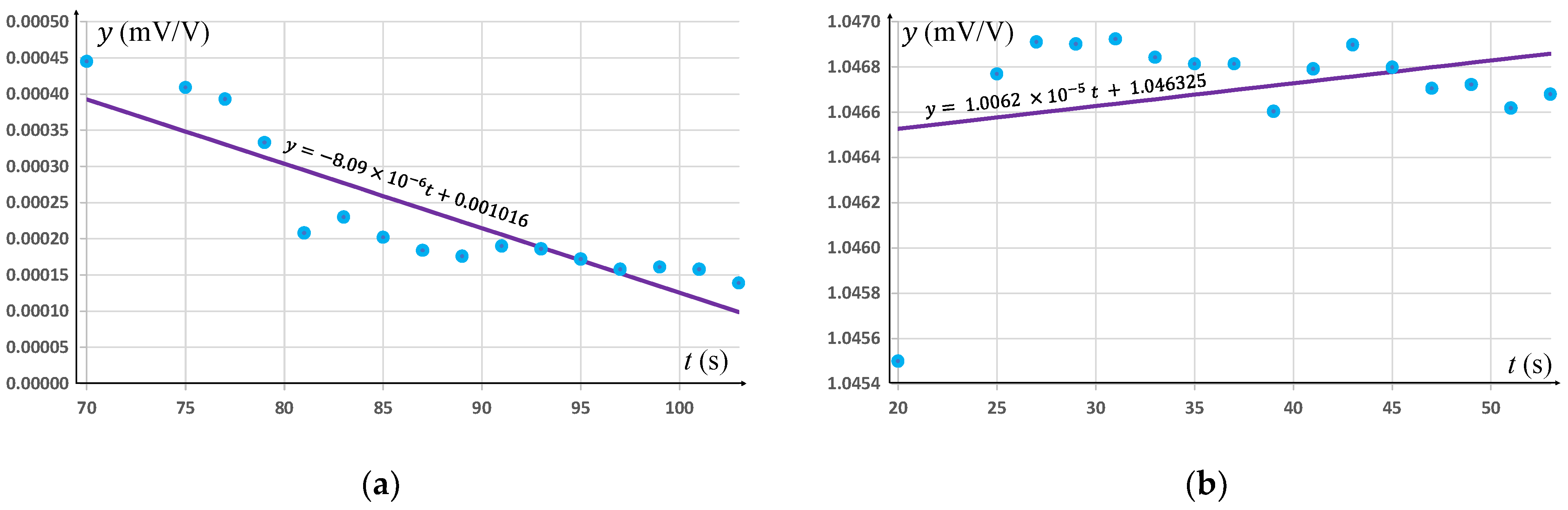
For the second more general case of fit with constant uncertainties u(t_i) = 0.3 s and u(y_i) = 0.0001 mV/V, method WTLS for straight line has been applied. Almost identical solutions were obtained, as in the first case:

• For adjustments of the low level of signal, diagram of a straight line in Figure 6a: y = −8.09 × 10⁻⁶ t + 0.001016with the value of the criterion function ϕ_ytmin = 3.36;
• For adjustments of the low level of signal, diagram of a straight line in Figure 6b: y = 1.0062 × 10⁻⁵ t + 1.046325 with the value of the criterion function ϕ_ytmin = 141.66.

8. Third-Degree Curve Adjustments by y = b₂t³ + b₁t + b₀

Third-degree curve adjustments y = b₂t³ + b₁t + b₀ have been implemented, taking into account only constant uncertainty values. In the first approach, condition (5) assumes the signal uncertainty constants u(y_i) = 0.0001 mV/V, and analytical solutions have been used (9, 10). In the second approach, an approximate solution was used for Equation (4) for uncertainty constants u(t_i) = 0.3 s and u(y_i) = 0.0001 mV/V (algorithm in 5.1).

In the first case, with constant signal uncertainty, the following relationships have been obtained:

• For adjustments of the low level of signal y = 1.53 × 10⁻⁹ t³ − 4.32 × 10⁻⁵ t + 0.003 05 with the value of the criterion function ϕ_tymin ≈ 1.37;
• For adjustments of the high level of signal y = −2.1 × 10⁻⁸ t³ + 1.01 × 10⁻⁴ t + 1.044234 with the value of the criterion function ϕ_tymin ≈ 88.32.

In the second case, with constant uncertainty of signal and time, the following relationships have been obtained:

• For adjustments of the low level of signal y = −5.02 × 10⁻¹⁰ t³ + 2.54 × 10⁻⁶ t + 3.633 × 10⁻⁴ with the value of the criterion function ϕ_ξymin ≈ 4.9;
• For adjustments of the high level of signal y = −2.9 × 10⁻⁸ t³ + 1.4 × 10⁻⁴ t + 1.0433 with the value of the criterion function ϕ_ξymin ≈ 75.7.

The above relationships for the adjustment of the measurement points for the lower level are illustrated (Figure 7).

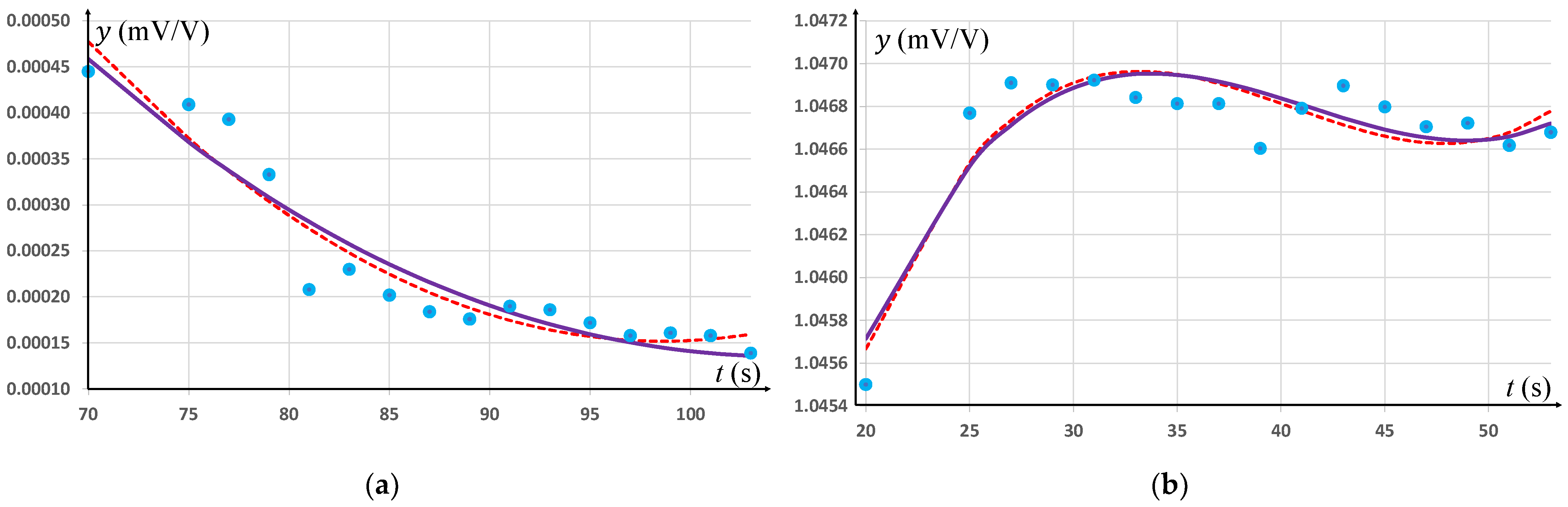
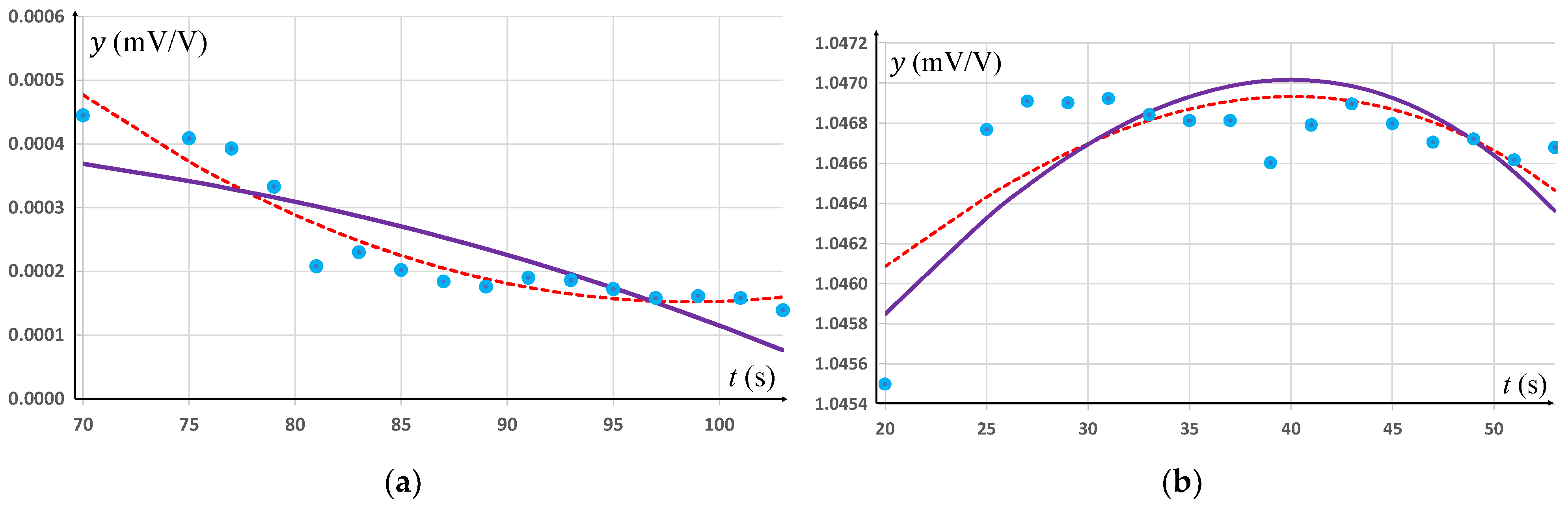
9. Third-Degree Curve Adjustments by y = a₃t³ + a₂t² + a₁t + a₀

Third-degree curve adjustments given by dependence y = a₃t³ + a₂t² + a₁t + a₀ have been implemented, taking into account only constant uncertainty values. In the first approach, in Equation (5), the signal uncertainty constants have been assumed to be u(y_i) = 0.0001 mV/V, and analytical solutions have been used (12, 13). In the second approach, an approximate solution to Equation (4) has been applied for uncertainty constants u(t_i) = 0.3 s and u(y_i) = 0.0001 mV/V using the algorithm in 5.1.

In the first case, with constant signal uncertainty, the following relationships have been obtained:

• For adjustments of the low level of signal y = 2.6 × 10⁻¹⁰ t³ + 4.67 × 10⁻⁷t² − 8.45 × 10⁻⁵t + 0.004193 with the value of the criterion function ϕ_tymin = 1.37;
• For adjustments of the high level of signal y = 2.12 × 10⁻⁷t³ − 2.58 × 10⁻⁵ t² + 1.01 × 10⁻³t + 1.034075 with the value of the criterion function ϕ_tymin = 29.55.

In the second case, with constant uncertainty of signal and time, the following relationships have been obtained:

• For adjustments of the low level of signal y = −9.22 × 10⁻¹⁰ t³ + 5.20 × 10⁻⁷ t² − 7.88 × 10⁻⁵t + 0.003742 with the value of the criterion function ϕ_ξymin = 1.55;
• For adjustments of the high level of signal y = 1.79 × 10⁻⁷ t³ − 2.23 × 10⁻⁵ t² + 8.89 × 10⁻⁴ t + 1.035436 with the value of the criterion function ϕ_ξymin ≈ 26.13.

The relationships in both the first case (the dashed curves of the third degree) and in the second case (the purple continuous curve) are illustrated (Figure 8).

10. Signal Average Estimators of Low and High Level

On the basis of the measurement points for the upper and lower levels, as well as the adjusted linear relationship described by the polynomial function of the third degree, a set of estimators was prepared for the measurement of the average value of the torque (presented in

Table 2. Signal average estimators.

Name	Symbol	Formula
Arithmetic mean	$\overline{y}$	$\frac{1}{n}{\displaystyle \sum _{i=1}^n}{y}_i$
Median	$y_M$	$\frac{y_{j=n/2}+y_{j=n/2+1}}{2}$
Middle of spread	$y_R$	$\frac{y_{\mathrm{m}\mathrm{i}\mathrm{n}}+y_{\mathrm{m}\mathrm{a}\mathrm{x}}}{2}$
Weighted average	${\overline{y}}_W$	${\displaystyle \sum _{i=1}^n}{t}_i{y}_i/{\displaystyle \sum _{i=1}^n}{t}_i$
Means from integration over time	$<y{>}_t$	$\frac{1}{{t_n-t}_1} \underset{t_1}{\overset{t_n}{\int }}f\left(t\right)dt$
Mean over time integration 1	$<y{>}_{\mathrm{t}\mathrm{p}1}$	$a\frac{t_1+t_n}{2}+b$
Mean over time integration 2	$<y{>}_{\mathrm{t}\mathrm{p}2}$	$\frac{t_1+t_n}{2}\left(\frac{b_3}{2}\left(t_1^2+t_n^2\right)+b_1\right)+b_0$
Mean over time integration 3	$<y{>}_{\mathrm{t}\mathrm{p}3}$	$\frac{t_1+t_n}{2}\left(\frac{a_3}{2}\left(t_1^2+t_n^2\right)+a_1\right)+\frac{a_2}{3}\left(t_1^2+t_1{t}_2+t_n^2\right)+a_0$

).

Table 2 shows the estimators of average values determined for both levels of the measured low and high signals.

From the above tables, it can be seen that from

Table 3. Values of the mean signal level and difference estimators.

(a)
Level/Level Difference	$\overline{y}$		$y_M$	$y_R$	${\overline{y}}_W$
Level 0 kN·m (mV/V)	0.000234		0.000188	0.000292	0.000225
Level 2000 N·m (mV/V)	1.046705		1.046708	1.046090	1.046729
Level 2000–Level 0 (mV/V)	1.046471		1.046520	1.045798	1.046504
(b)
Level/Level Difference	$<y{>}_{\mathrm{t}\mathrm{p}1}$		$<y{>}_{\mathrm{t}\mathrm{p}2}$		$<y{>}_{\mathrm{t}\mathrm{p}3}$
	u($y_i$) = 0.0001	u($t_i$) = 0.3 u($y_i$) = 0.0001	u($y_i$) = 0.0001	u($t_i$) = 0.3 u($y_i$) = 0.0001	u($y_i$) = 0.0001	u($t_i$) = 0.3 u($y_i$) = 0.0001
Level 0 kN·m (mV/V)	0.000246	0.000316	0.000343	0.000246	0.000594	0.000246
Level 2000 N·m (mV/V)	1.047195	1.046692	1.046693	1.046700	1.046688	1.046690
Level 2000–Level 0 (mV/V)	1.046949	1.046376	1.046350	1.046454	1.046094	1.046444

(a) that the median resistant to outliers and the weighted average emphasizing the final, practically established values of the sampled signal under equilibrium conditions (mean 1.0465 mV/V) are the most similar to each other. The center of the span and the arithmetic mean stand out significantly from this level. On the other hand, Table 3 (b) shows that the mean of the integration of the most fitted third-degree curve (tp3), taking into account the uncertainty of time and signal, differs by less than 0.000 08 mV/V. Similarly close to this solution is the polynomial curve (tp2) below 0.000 01 mV/V. On the other hand, the fit of the trend line (tp1) gives the differences between the estimated means above 0.0001 mV/V.

11. Signal Variance Value Estimators

In order to determine the coverage interval and, above all, the standard uncertainty, the following definitions of variance were used.

11.1. Arithmetic Mean Variance Estimator

This estimator is the equal square of the standard deviation of the experimental mean, dedicated to the gaussian distributions [21,38]:

$$u_{EA}^2(y)=\frac{1}{n\left(n-1\right)}\sum _{i=1}^n{{(y}_i-\overline{y})}^2$$

(19)

11.2. Estimator of Variance for Middle of Spread

This estimator is equal to the square of uncertainty determined as the maximum error estimated by the arithmetic mean from the difference between the maximum and minimum of the y value (the maximum error for a rectangular distribution) [21,39]:

$$u_R\left(y\right)=\frac{y_{\mathrm{m}\mathrm{a}\mathrm{x}}{-y}_{\mathrm{m}\mathrm{i}\mathrm{n}}}{2\sqrt{3}}$$

(20)

11.3. Allan Variance Estimator

This estimator is equal to the square of the uncertainty determined by half of the sum of the squares of the individual measurements (the means of the measurements) [40]:

$$u_A^2(y)=\frac{1}{2\left(n-1\right)}\sum _{i=1}^{n-1}{{(y}_i-y_{i+1})}^2$$

(21)

11.4. Variance Estimator for Integral Mean

This estimator is equal to the square of uncertainty determined by the mean uncertainty corridor around the line y = θ₁ξ + θ₀, where the variance for a line is given by σ² = u²(θ₁) ξ² + 2ρ_θ1θ0 ξ u(θ₀) u(θ₁) + u²(θ₀). This estimator, fitted to, in general, a nonlinear curve and averaged over time is equal to:

$$<u^2{>}_t=\frac{1}{{t_n-t}_1}{\int }_{t_1}^{t_n}{[u}^2\left({\theta }_1\right){\xi }^2\left(t\right)+2{\rho }_{{{\theta }_0\theta }_1}\xi \left(t\right)u\left({\theta }_1\right)u\left({\theta }_0\right)+u^2\left({\theta }_0\right)] \mathrm{d}t$$

(22)

• Case tp1. Straight line fit

For the equation of a line $y=at+b,$ function $\xi \left(t\right)=t$ and parameters ${\theta }_1=a, {\theta }_0=b$. Then, the result from Formula (22) is as follows:

$$<u_{p1}^2{>}_t=u^2\left({\theta }_1\right){(t}_1^2+t_1{t}_n+t_n^2)/3+{\rho }_{{{\theta }_0\theta }_1}u\left({\theta }_1\right)u\left({\theta }_0\right)({t_n+t}_1)+u^2\left({\theta }_0\right)$$

(23)

Variance values u²(θ₁) i u²(θ₀) and covariance element ρ_θ1θ0 u(θ₀)u(θ₁) for variables θ₁ and θ₀ are determined numerically from the law of uncertainty propagation using the matrix L ${\mathit{U}}_{\mathit{T}\mathit{S}}$L after adjusting the curve parameters and obtaining the global minimum of the criterion function. After linearization of the model, the slope θ₁ and intercept θ₀ are linearly dependent on the time and signal coordinates. It is necessary to determine the matrix of the sensitivity coefficients by numerically differentiating the increments for both parameters and calculating appropriate differential quotients with the use of appropriately selected increments of time and signal coordinates. A bilaterally multiplied matched covariance matrix by a sensitivity coefficient matrix (right-hand transposed) leads to the determination of the variances and covariances contained in the formula (23).

• Case tp2. Fitting a Third-Order Polynomial Curve

For a polynomial y = b₂ t³ + b₁ t + b₀, the function in (22) is determined by the ξ(t) = t³ + β₁t, and parameter β₁ = b₁/b₂, and the parameters of a straight line θ₁ = b₂, θ₀ = b₀.

The time-average value of the variance after integration is:

$$\begin{gathered} {<u}_{p2}^2{>}_t=u^2\left({\theta }_1\right)(W_7/7+({2b}_1/b_2)W_5/5+{{(b}_1/b_2)}^2{W}_3/3) \\ +{\rho }_{{{\theta }_0\theta }_1}u\left({\theta }_1\right)u\left({\theta }_0\right){(W_4/2+b}_1{W}_2/b_2)+u^2\left({\theta }_0\right) \end{gathered}$$

(24)

where this is denoted by

$$W_k=\frac{{\left(t_n\right)}^k-{\left(t_1\right)}^k}{t_n-t_1}=\sum _{j=0}^k{\left(t_1\right)}^j{\left(t_n\right)}^{k-j}$$

(25)

• Case tp3. Fitting a Third-Order Polynomial Curve

For a polynomial $y=a_3{t}^3+a_2{t}^2+a_{1}t+a_o,$ the function in (22) is $\xi \left(t\right)=t^3+{{\beta }_{1}t}^2+{\beta }_{2}t, {\beta }_1=\frac{a_2}{a_3}$, ${\beta }_2=\frac{a_1}{a_3}$, and the parameters of the straight line ${\theta }_1=a_3,{\theta }_0=a_o$. The time-averaged value of variance after integration (22) is:

$$\begin{array}{cc}\hfill {<u}_{p3}^2{>}_t=u^2\left({\theta }_1\right)& (W_7/7+a_2{W}_6/(3a_3)+(({a_2/a_3)}^2+{2a}_1/a_3)W_5/5\hfill \\ & +{(a}_1{a}_2{/2)W}_4/{\left(a_3\right)}^2+{{(a}_1/a_3)}^2{W}_3/3)+{\rho }_{{{\theta }_0\theta }_1}u\left({\theta }_1\right)u\left({\theta }_0\right)(W_4/2\hfill \\ & +2a_2{W}_3/({3a}_3)+a_1{W}_2/a_3)+u^2\left({\theta }_0\right)\hfill \end{array}$$

(26)

In the first place, the values of the covariance matrix for the simple y = ${\theta }_1\xi +{\theta }_0$. These values for the different fit curves are shown in

Table 4. The uncertainties of the estimated parameters of the straight line y = ${\theta }_1\xi +{\theta }_0$.

Type of Function $\mathsf{\xi }\left(\mathit{t}\right)$	Torque	$\mathit{u}\left({\mathsf{\theta }}_{\mathbf{1}\mathbf{m}\mathbf{i}\mathbf{n}}\right)$	$\mathbf{u}\left({\mathsf{\theta }}_{\mathbf{0}\mathbf{m}\mathbf{i}\mathbf{n}}\right)$	${\mathsf{\rho }}_{{{\mathsf{\theta }}_{\mathbf{0}}\mathsf{\theta }}_{\mathbf{1}}}$
$\xi \left(t\right)=t$	0	1.4 × 10−5 mV/sV	0.0012 mV/V	−1
$\xi \left(t\right)=t$	2000	3.5 × 10−5 mV/sV	0.0013 mV/V	−1
$\xi \left(t\right)=t^3+{{\beta }_{1}t}^2$	0	1.3 × 10−10 mV/s3V	0.000 04 mV/V	−0.8
$\xi \left(t\right)=t^3+{{\beta }_{1}t}^2$	2000	2.4 × 10−9 mV/s3V	0.000 28 mV/V	−1
$\xi \left(t\right)=t^3+{{\beta }_{1}t}^2+{\beta }_{2}t$	0	2.5 × 10−10 mV/s3V	0.001 mV/V	−1
$\xi \left(t\right)=t^3+{{\beta }_{1}t}^2+{\beta }_{2}t$	2000	1.7 × 10−8 mV/s3V	0.001 mV/V	−1

.

On the basis of the elements of the covariance matrix, the estimators from Formula (22) for simple Formula (23) and two polynomials fitted by the third degree—Formulas (24) and (25)—for the low and high levels have been determined. All the proposed variance estimators in the form of square roots as standard uncertainties have been determined and are compiled in

Table 5. Estimator of standard deviation: the uncertainties of low and high levels.

Type of Uncertainties	Estimated Value for 0 kN·m ${\mathsf{u}}_{\mathit{L}}$ (mV/V)	Estimated Value for 2000 N·m ${\mathsf{u}}_{\mathit{H}}$ (mV/V)	Estimated Value for Difference $\sqrt{{\mathsf{u}}_{\mathit{L}}^{\mathbf{2}}\mathbf{+}{\mathsf{u}}_{\mathit{H}}^{\mathbf{2}}}$ (mV/V)
$u_{EA}\left(y\right)$	2.5 × 10−5	8.4 × 10−5	8.8 × 10−5
$u_R\left(y\right)$	2.89 × 10−5	3.41 × 10−5	4.45 × 10−5
$u_A\left(y\right)$	2.8 × 10−5	2.42 ×10−4	2.4 × 10−4
$u_{p1}=\sqrt{<u_{p1}^2{>}_t}$	1.34 × 10−4	3.34 × 10−4	3.6 × 10−4
$u_{p2}=\sqrt{<u_{p2}^2{>}_t}$	3.3 × 10−5	4.5 × 10−4	4.5 × 10−4
$u_{p3}=\sqrt{<u_{p3}^2{>}_t}$	5.8 × 10−5	7.37 × 10−5	9.4 × 10−5

.

12. Discussion

As a result, the standard uncertainty estimators for the actual signal level corresponding to the measured torque of 2 kN·m were numerically calculated. When constructing estimators based on the fitted time signal function, the least squares method was employed to minimize the criterion function with zero uncertainty in time measurement, ensuring accurate time measurement. Additionally, when accounting for uncertainties in both variables (signal and time of measurement points), analytical formulas for the parameters of the fitted curves were used in conjunction with the ordinary least squares (OLSs) method. The fit model, considering the uncertainty of both variables, was quantitatively solved using the weighted least squares (WLS) method, which minimized the criterion function. The solutions obtained for both cases exhibited slight differences for the polynomial fit, as illustrated in Figure 5 and Figure 6.

In the WLS method, the averaging of the solution was achieved by incorporating uncertainty, resulting in signal-level estimators for both the expected value and the standard uncertainty. Notably, higher values of uncertainty were observed for an incomplete polynomial of third degree (type I, tp2) and for a straight line fit (tp1). Conversely, lower uncertainty values were obtained for the middle of spread variance and experimental deviation from average variance. The use of Allan variance in the estimation of quartz time oscillator time showcased similar trends, with more than twice smaller values compared to the Allan deviation for fitting the full parameters of a polynomial of the third degree (type II, tp3). The smallest uncertainty values were attained for the experimental deviation of the mean and the arithmetic mean of the most scattered points.

13. Conclusions

Algorithmic approaches for analyzing creep study in measuring torque transducer were proposed. An algorithm of approximate polynomial fit–straight line, a polynomial of the third degree to a series of points determined at intervals, is presented. Fit parameters and an averaged corridor of uncertainty were determined.

This article provides an analysis of the metrological properties of the creep process during the calibration of the torque transducer. The relative electrical signal (given in electrical units, mV/V) as a function of torque measured was monitored at intervals of time. To fit the data, the weighted method of least squares with both a straight line and a cubic spline curve was used to measure low and high levels of transducer in static measurement. To find the estimated measurand value at 2 kN·m and 0 kN·m, a few estimators of averages (arithmetical, middle spread, average of integral) have been applied, as well as for estimators of deviation like experimental deviation, Allan’s spread, and the integral average of coverage corridor. In the results, we chose the appropriate estimators for the average of the signal and uncertainty, which are not typical statistical estimators. Due to the mechanical similarity of the tested 2 kN·m torque transducer to the 5 MN·m torque transducer, the proposed algorithms may be useful for optimizing the creep signal and its uncertainty for mechanically similar transducers.

In conclusion, torque transducers are vital components in wind energy applications, enabling the measurement of torque data critical for power optimization and turbine performance analysis. Various parameters, including temperature, applied load, calibration frequency, and environmental factors, influence the creep behavior of these transducers. Understanding and considering these parameters allows for accurate and reliable measurements, ensuring the efficient and safe operation of wind turbines.

By performing data-driven analyses, researchers can uncover correlations between various environmental conditions, operational parameters, and creep behavior in torque transducers. Determining the disparity in the magnitude of the upper and lower signals, along with precisely estimating the associated uncertainty, plays a critical role in establishing the accurate and typically linear attributes of the transducer, alongside its corridor of uncertainty. This knowledge can help optimize the design and implementation of torque transducers in wind energy systems. For instance, the analysis may reveal that specific wind speeds or temperature ranges significantly influence creep, leading to adjustments in the turbine’s operating parameters or torque transducer materials and designs.

Algorithms and AI methods, such as the Kalman filter and artificial neural networks, offer powerful tools for analyzing and compensating for creep effects in torque measurements of wind turbines, enabling the accurate estimation of true torque values and facilitating proactive maintenance interventions and the early detection of potential failures.