Abstract
This paper reviews the application of artificial neural network (ANN) models to time series prediction tasks. We begin by briefly introducing some basic concepts and terms related to time series analysis, and by outlining some of the most popular ANN architectures considered in the literature for time series forecasting purposes: feedforward neural networks, radial basis function networks, recurrent neural networks, and self-organizing maps. We analyze the strengths and weaknesses of these architectures in the context of time series modeling. We then summarize some recent time series ANN modeling applications found in the literature, focusing mainly on the previously outlined architectures. In our opinion, these summarized techniques constitute a representative sample of the research and development efforts made in this field. We aim to provide the general reader with a good perspective on how ANNs have been employed for time series modeling and forecasting tasks. Finally, we comment on possible new research directions in this area.
1. Introduction
Predictions can have great importance on various topics, like birthrates, unemployment rates, school enrollments, the number of detected influenza cases, rainfall, individual blood pressure, etc. For example, predictions can guide people, organizations, and governments to choose the best options or strategies to achieve their goals or solve their problems. Another example of the application of predictions can be found in the consumption of electrical energy to guarantee the optimal operating conditions of an energy network that supplies electrical energy to its customers [1,2,3,4,5]. A time series is a set of records about a phenomenon that is ordered equidistantly with respect to time; this is also called a forecast. Time series are used in a wide variety of areas, including science, technology, economics, health, the environment, etc. [6]. Initially, statistical models were used to forecast the future values of the time series. These models are based on historical values of the time series to extract information about patterns (trend, seasonality, cycle, etc.) that allow the extrapolation of the behavior of the time series [1].
We can identify in the literature two main classes of methodologies for time series analysis:
- Parametric statistical models. Among the traditional parametric modeling techniques, we have the autoregressive integrated moving average (ARIMA) linear models [7]. The 1970s and 1980s were dominated by linear regression models [8].
- Nonparametric statistical models. Some of these techniques include the following: self-exciting threshold autoregressive (SETAR) models [9], which are a nonlinear extension to the parametric autoregressive linear models; autoregressive conditional heteroskedasticity (ARCH) models [10], which assume that the variance of the current error term or innovation depends on the sizes of previous error terms; and bilinear models [11], which are similar to ARIMA models, but include nonlinear interactions between AR and MA terms.
The main difference between both classes is that the parametric model has a fixed number of parameters, while the nonparametric model increases the number of parameters with the amount of training data [12].
Although nonlinear parametric models represent an advance over linear approaches, they are still limited because an explicit relational function must be hypothesized for the available time series data. In general, fitting a nonlinear parametric model to a time series is a complex task since there is a wide possible set of nonlinear patterns. However, technological advancements have allowed researchers to consider more flexible modeling techniques, such as support vector machines (SVMs) adapted to regression [13], artificial neural networks (ANNs), and wavelet methods [14].
McCulloch and Pitts [15] and Rosenblatt [16] established the mathematical and conceptual foundations of ANNs, but these nonparametric models really took off in the late 1980s, when computers were powerful enough to allow people to program simulations of very complex situations observed in real life, generated by simple and easy-to-understand stochastic algorithms that nevertheless demanded intensive computing power. ANNs belong to this class of simulations since they are capable of modeling brain activity in classification and pattern recognition problems. It was demonstrated that ANNs are a good alternative to time series forecasting. In 1987, Lapedes and Farber [17] reported the first approach to modeling nonlinear time series with an ANN. ANNs are an attractive and promising alternative for several reasons:
- ANNs are data-driven methods. They use historical data to build a system that can give the desired result [18].
- ANNs are flexible and self-adaptive. It is not necessary to make many prior assumptions about the data generation process for the problem under study [18].
- ANNs are able to generalize (robustly). They can accurately infer the invisible part of a population even if there is noise in the sample data [19].
- ANNs can approximate any continuous linear or nonlinear function with the desired accuracy [20].
The aim of this review is to provide the general reader with a good perspective on how ANNs have been employed to model and forecast time series data. Through this exposition, we explore the reasons why ANNs have not been widely adopted by the statistical community as standard time series analysis tools. Time series modeling, specifically in the field of macroeconomics, is limited almost exclusively to methodologies and techniques typical of the linear model paradigm, ignoring completely machine learning and artificial neural network techniques, which have effectively produced time series forecasts that are more accurate in comparison to what linear modeling has to offer. This paper (a) introduces ANNs to readers familiar with traditional time series techniques who want to explore more flexible and accurate modeling alternatives, and (b) illustrates recent techniques involving several ANN architectures chiefly employed with the goal of improving time series prediction accuracy.
The rest of this document is organized as follows: Section 2 introduces basic time series analysis concepts. In Section 3, we outline some of the most popular ANN architectures considered in the state-of-the-art for time series forecasting; we also analyze the strengths and weaknesses of these architectures in the context of time series modeling. In Section 4, we provide a brief survey on relevant time series ANN modeling techniques, discussing and summarizing recent research and implementations. Section 5 provides a discussion on the application of ANN in time series forecasting. Finally, in Section 6, we discuss possible new research directions in the application of ANN for time series forecasting.
2. Basic Principles and Concepts in Time Series Analysis
In this section, we define, more or less formally, what a time series is (Section 2.1); then, we discuss how a time series forecast can be analyzed as a functional approximation problem (Section 2.2). This approach will enable us to construct mathematical models aimed at predicting future time series values. We close this section by briefly describing what an ARIMA model is, how ARIMA models are employed for time series predictions, and why they are popular among statisticians and practitioners (Section 2.3).
2.1. What Is a Time Series?
A time series can be represented as a sequence of scalar (or vector) values , , …, corresponding to contiguous, equally spaced points in time labeled (e.g., we could measure one value each second, or each hour, or each week, or each month, etc., depending on the nature of the process, on the available technology to measure and store data, and on how we plan to use the collected data); this labeling convention does not depend on the frequency at which values are sampled from a real-world process.
Nowadays, time series have an impact in various fields. For example, they occur daily in economics, where currency quotes are recorded in time periods of minutes, hours, or days. Governments publish unemployment, inflation, or investment figures monthly. Educational institutions maintain annual records of school enrolment, dropout rates, or graduation rates [21]. Recently, international health organizations published the number of people who were infected by or deceased due to the COVID-19 pandemic daily. Several industries record the number of failures that occur per shift in production lines to determine the quality of their processes.
Time series forecasting involves several problems that complicate the task of generating an accurate prediction; for example, missing values, noise, capture errors, etc. Therefore, the challenge is to isolate useful information from the time series, eliminating the aforementioned problems to achieve a forecast [22].
2.2. Time Series Modeling
As mentioned above, time series analysis focuses on modeling a phenomenon y from time t backwards , with the objective of forecasting the following values of y up to a prediction horizon s. For predicting , one can assume a functional model f based on the historical records , , , …, :
Equation (1) is a function approximation problem, and it can be solved by applying the following steps (see [23]):
- Functional model f: Suppose a function f that represents the dependence of related to ;
- Training phase: For each past value , train f using as inputs the values , and …, , and as target ;
- Predict value : Apply the trained functional model f to predict from , , , …, .
The training phase step should be repeated until all predictions are close enough to their corresponding target values . If the functional model f is properly trained, it will produce accurate forecasts, . The above steps can be applied to forecast any horizon s, replacing with as the target. The three-step procedure presented above is known as an autoregressive (AR) model.
2.3. ARIMA Time Series Modeling
In 1970, Box and Jenkins [7] popularized the autoregressive integrated moving average (ARIMA) model, which is based on the general autoregressive integrated moving average (ARMA) model described by Whittle [24].
In Equation (2), the first term represents the autoregressive (AR) part, and the second term represents the moving average (MA) part. The terms represent white noise. Typically, are assumed to be random variables that come from a normal distribution . The parameters and are estimated from the historical values of the time series. We can estimate at time as .
The ARIMA model is an improvement on the ARMA model for dealing with non-stationary time series with trends. The SARIMA model is an extension of the ARIMA model for dealing with data with seasonal patterns; for more information, please consult Shumway and Stoffer [21].
Models from the ARIMA family suppose that the time series is generated from linear, time-invariant processes; this assumption is not valid for many situations. Nevertheless, up to now, the ARIMA model and its variants have continued to be very popular; for instance, they are used by most official statistical agencies around the world as an essential part of their modeling strategy when working with macroeconomic or ecological/environmental temporal data. The popularity of ARIMA modeling stems from the following facts:
- Linear modeling is always at the forefront of the literature;
- Linear models are easy to learn and implement;
- Interpretation of results coming from linear models relies on well-defined, well-developed, standardized, mechanized procedures with solid theoretical foundations (e.g., there are established procedures that help us build confidence intervals associated with point forecasts, founded on statistical and probabilistic theory centered around the normal distribution).
On the other hand, when phenomena require the investigation of alternative nonlinear time series models, it is useful to consider the following comment by George E. P. Box:
Since all models are wrong, the scientist cannot obtain a “correct” one by excessive elaboration; on the contrary, following William of Occam, he should seek an economical description of natural phenomena. Just as the ability to devise simple but evocative models is the signature of the great scientist, so over-elaboration and over-parametrization is often the mark of mediocrity.(Box [25], 1976)
Occam’s razor (a principle also known as parsimony) is often used to avoid the danger of overfitting the training data, that is, to choose a model that perfectly fits the time series data but is very complex and hence often does not generalize well. Time series analysis sometimes follows this principle in that many ARIMA or SARIMA models perform increasingly worse as the number of historical values used to forecast increases [26].
3. Popular ANN Architectures Employed for Time Series Forecasting Purposes
As mentioned previously in Section 1, artificial neural networks (ANNs) belong to the class of nonlinear, nonparametric models; they can be applied to several pattern recognition, classification, and regression problems. An ANN is a set of mathematical functions inspired by the flow of electrical and chemical information within real biological neural networks. Biological neural networks are made up of special cells called neurons. Each neuron within the biological network is connected to other neurons through dendrites and axons (neurons transmit electrical impulses through their axons to the dendrites of other neurons; the connections between axons and dendrites are called synapses). An ANN consists of a set of interconnected artificial neurons. Figure 1 shows a graphical representation of a set of neurons interconnected by arrows, which helps us see how information is processed within an ANN.

Figure 1.
Single hidden layer feedforward neural network.
In this section, we are going to briefly describe the basic aspects of some popular ANN architectures commonly employed for time series forecasting: feedforward neural networks (FFNNs), radial basis function networks (RBFNs), recurrent neural networks (RNNs), and self-organizing maps (SOMs). As we advance in our discussion of FFNNs, occasionally we will encounter some specific concepts needed to transform an FFNN into a time series forecasting model; most of these additional concepts are also applicable to the remaining ANN architectures considered in this section. Comments in Section 3.2, Section 3.4, and Section 3.5 are based on material found in an online course prepared by Bullinaria [27]. In turn, this online material is based on the following textbooks: Beale and Jackson [28], Bishop [29], Callan [30], Fausett [31], Gurney [32], Ham and Kostanic [33], Haykin [34], and Hertz [35].
3.1. Feedforward Neural Networks
3.1.1. Basic Model
Also known in the state of the art by the name of multilayer perceptron (MLP), a feedforward neural network (FFNN), is an ANN architecture where information flows in one direction only, from one layer to the next. Typically, an FFNN is composed of an input layer, one or more hidden layers, and an output layer. In each hidden layer and the output layer, there are neurons (nodes) that are usually connected to all the neurons in the next layer. Figure 1 shows a single FFNN hidden layer with inputs and output .
In the structure shown in Figure 1, information is transmitted from left to right; the inputs , , …, are transformed into the output . In the context of time series modeling, focusing on the AR model, FFNN inputs , , …, correspond to time series values , , , …, , while FFNN output typically corresponds to a prediction value , which attempts to approximate future time series value (see Section 2.2).
Each arrow in the FFNN structure in Figure 1 represents a weight w for the input value x that enters on the left of the arrow, and exits on the right side with the value . The input layer is formed by the independent variables , , …, and a constant value known as the intercept. For each neuron, all its inputs are summed, and then this sum is transformed by applying a nonlinear activation function . One of the most-used activation functions in ANNs is the logistic (sigmoid) function . The hyperbolic tangent is another frequently used activation function . The functionality of each neuron in the hidden layer h is described by
where each represents the weight that corresponds to the arrow that connects the input node with the neuron h. In Figure 1, the output layer contains only one neuron; this is the number of output units needed if we are interested in predicting a single scalar time series value, but we can employ more output units if we need multiple prediction horizons (scalar or vector). Neurons in an output layer have identical functionality to those in hidden layers, although output neurons sometimes employ the identity function as an activation function (especially for time series forecasting tasks). It is also possible, however, to use as an activation function for output units the same sigmoidal activation functions employed by hidden units (i.e., logistic or hyperbolic tangent). It is even possible to employ different activation functions for units in the same layer. The output layer functionality for our FFNN, depicted in Figure 1, assuming an identity activation function, is described by
3.1.2. FFNN Training
In summary, the ANN has a set of parameters that must be set to determine how the input data are processed and the output generated: weights and biases. The weights are related to the control of the connection between two neurons. The weight value determines the magnitude and direction of the impact of a given input on the output. Biases can be defined as the constant that is added to the product of features and weights. It helps models change the activation function to the positive or negative side [36].
FFNNs are trained, or “taught”, with the help of supervised machine learning algorithms. Backpropagation (BP) is probably the most popular machine learning algorithm employed to train FFNN models. Next, we describe briefly how BP works. The idea is to adjust all weights and biases in the FFNN model so that, in principle, they minimize some fitting criterion E; for example, the mean squared error:
where n is the number of example input patterns available for training our model, is the target (desired value) for the pth example input pattern, and is the FFNN output also for the pth example input pattern, . FFNN weights are adjusted according to the backpropagation rule: , where meta-parameter is a small positive number called “learning rate”, is a vector containing all FFNN weights, and w is a single FFNN weight (i.e., w can be any single component of ). Basically, the BP algorithm consists of the following steps:
- Initialize randomly;
- Repeat (a) and (b) until is below a given threshold T or a pre-established maximum number of iterations M has been reached:
- (a)
- ;
- (b)
- Update all network weights: ;
- Return .
From this algorithm outline, we see that BP starts from a random point in search space W and looks for the global minimum of the error surface , say , by taking small steps, each towards a direction opposite to the derivative (gradient) of the multivariate error function E, evaluated at the current location in the search space W where BP has advanced so far. If is smooth enough, BP will descend monotonically when moving from one step to the next; this is why BP is said to be a stochastic gradient descent procedure.
In summary, the goal of BP is to iteratively adjust , applying the gradient descent technique, so that the output of the FFNN is close enough to the target values in the training data [29]. For convex error surfaces, BP would do a nice job; unfortunately, often contains local minima, and in such situations, BP can easily become stuck into one of those minima. A heuristic approach to facing this issue is to run BP several times, keeping all FFNN settings fixed (e.g., set of training data, number of inputs d, number of hidden neurons q, and BP meta-parameters).
Another important issue we face when training FFNNs with BP is that of overfitting. This condition occurs when a model adapts too well to the local stochastic structure of (noisy) training examples but produces poor predictions for inputs not in the training examples. If we strictly aim for global minimum, then we focus only on interpolating exactly all training data examples. In most situations, however, we would like to use our FFNN model for predicting, as accurately as possible, y values corresponding to unseen (although fairly similar to training examples) inputs , i.e., we would like our FFNN model to have small prediction error (prediction error can be measured much like training error E using, for example, the mean squared error once the unseen future values become available). Note that the true prediction error cannot be measured simultaneously with the training error during the BP process, but we can estimate the former if we reserve some training examples as if they were future inputs (see Section 3.1.5).
From all of this, we conclude that reaching global minimum, in fact, should not be our main objective when training an FFNN for prediction purposes; we should instead employ heuristic techniques in order to improve the prediction (generalization) ability of our FFNN model. A simple heuristic approach is to use early stopping, so that BP becomes close, but not too close, to the global minimum . Another possibility is to employ regularization. In this technique, we would incorporate, for instance, the term to our error function and run BP as usual. This would force BP to produce a smoother, non-oscillating output , thereby reducing the risk of over-fitting. Regularization penalizes FFNN models with large weights w and establishes a balance between bias and variance for the output .
3.1.3. Time Series Training Examples for FFNNs
The above description of FFNN training is very general, and thus, many questions arise. Specifically, when we attempt to teach an FFNN how to forecast future time series values, we face an obvious question: how do we arrange our available time series values into a set of training examples so that we are able to use BP or some other supervised machine learning algorithm? Suppose that we have N time series values at our disposal to train our FFNN model and we want to produce one-step-ahead forecasts. According to the autoregressive approach, the inputs to the FFNN model are the time series values , while the time series value is the target value. From our available time series data, we see that t can take values . Thus, a very simple way to build a training dataset for FFNN models intended to produce one-step-ahead univariate time series forecasts consists of rearranging available time series values in a rectangular array (see Table 1), where we fixed the number of inputs in our FFNN model to , so the first twelve columns contain values for predictor variables and the right column contains values for the (target) response variable . Each row in Table 1 represents an example of training that can be applied in conjunction with a supervised machine learning algorithm, such as BP.

Table 1.
Training dataset for one-step-ahead FFNN time series models.
3.1.4. FFNN Time Series Predictions
Now, suppose we want to predict still unavailable time series values , , …, using an FFNN model trained with the examples in Table 1 and designed to produce one-step-ahead forecasts. How do we achieve this task? To generate predicted values , first, we estimate using values as inputs to our FFNN model. Next, we predict using the values as inputs. Note that the most recently calculated model forecast is used as one of the inputs. To predict , the two most recently calculated forecasts are used as two of the model inputs. This iterative process continues until the forecast value is obtained.
3.1.5. Cross-Validation
Cross-validation (CV) is a statistical technique for estimating the prediction (or forecasting) accuracy of any model using only available training examples. CV can be helpful when deciding which model to select from a list of properly trained models; we would of course select the model that exhibits the smallest prediction error, as estimated by the CV procedure. CV can also serve as a training framework for ANNs; in fact, CV is often regarded as an integral part of the FFNN model construction process. In general, when training FFNNs for prediction purposes, CV is employed to fine-tune FFNN meta-parameters (such as d, the number of input nodes, and q, the number of hidden units), aiming at reducing over-fitting risk and at the same time improving generalization ability (i.e., prediction accuracy). The idea here is to regard a combination of meta-parameters, say , as a unique FFNN model. Following this idea, we would apply CV, for example, to each element in the combination set , generating an estimated CV prediction error for each one of the 12 possible combinations. We would finally keep the combination (i.e., FFNN model) that generates the smallest CV prediction error. So, how does CV work? Typically, we randomly split our set of available training examples into two complementary sets: one set, containing approximately 80% of all training examples, is used exclusively for training the considered model, while the other set, containing the remaining 20% of all training examples, is used exclusively for measuring prediction accuracy by comparing target values and their corresponding model outputs via an error function similar to that employed in BP to quantify training error, e.g., mean squared error. The former of these two complementary sets is obviously called the training set and the latter is called the validation set. The 80% and 20% sizes are just a rule of thumb, and other sizes for these two sets could be chosen. So, we use the training set to obtain a fully trained FFNN model via BP, for example, and then feed to this trained FFNN model the input values contained in the examples from the validation set, thus obtaining outputs that are compared against their corresponding target values from the validation set, producing a prediction error measure, . This is the basic CV iteration. We repeat many times the basic CV iteration (random generation computation) in order to generate many measures, and finally, we average all generated s. This final average would be the estimated prediction error produced by the CV procedure. As we can see, this is a procedure that makes intensive use of available computational resources but produces robust results. We can combine CV with regularization for even better results. For more information about CV, early stopping, regularization, and other techniques to improve FFNN performance, see Bishop [29].
It is important to keep in mind that to obtain valid results from the CV procedure, we must make sure that our training data examples are independent and come from the same population. Unfortunately, the condition of independence does not hold with time series data, as chronologically ordered observations are almost always serially correlated in time (one exception is white noise). To our knowledge, there is not currently a standard way of performing CV for time series data, but two useful CV procedures that deal with the issue of serial dependence in temporal data can be found in Arlot, Celisse, et al. [37,38]. Essentially, the modified CV procedure proposed by Arlot, Celisse, et al. [37] chooses the training and validation sets in such a way that the effects of serial correlation are minimized, while [38] proposes a procedure called forward validation, which exclusively uses the most recent training examples as validation data. CV error produced by the forward validation procedure would be a good approximation to unknown prediction error since the short-term future behavior of a time series tends to be similar to that of its most recently recorded observations.
3.1.6. FFNN Ensembles for Time Series Forecasting
FFNN models can be trained with stochastic optimization algorithms like BP, PSO, GA, etc. Because of this, FFNN models for time series prediction produce forecasts that depend on the result of the optimization that is being carried out. That is, the optimization process conditions the random variable . The above is true even when the optimization process always has the same initial conditions (the same training dataset and the same initial parameters). This stochastic prediction property of FFNN models, combined with their conceptual simplicity and their ease of training and implementation (relative to other ANN architectures), allows us to easily construct, from a fixed set of training examples, n independent FFNN models, collectively known as an FFNN ensemble. This FFNN ensemble model constructed produces, for a fixed time point t, a set of individual predictions in response to a single input pattern. Such individual predictions can then be combined in some way, e.g., by averaging, to produce an aggregate prediction that is hopefully more robust, stable, and accurate when compared against their individual counterparts. This basic averaging technique is similar to that found in Makridakis and Winkler [39]. It is important to emphasize here that prediction errors from individual ensemble components need to be independent, i.e., non-correlated or at least only weakly correlated, in order to guarantee a decreasing total ensemble error with an increasing number of ensemble members. FFNN ensemble models in particular fulfill this precondition, given the stochastic nature of their individual outputs. Additionally, all individual predictions could be used to estimate prediction intervals since the distribution of individual forecasts already contains valuable information about the model uncertainty and robustness. Barrow and Crone [40] average the individual predictions from several FFNN models that are generated during a cross-validation process, thus constructing an FFNN ensemble model aimed at producing robust time series forecasts. They compare their proposed strategy (called “crogging”) against conventional FFNN ensembles and individual FFNN models. They conclude that their crogging strategy produces the most accurate forecasts. From this, it could be argued that FFNN ensembles whose individual components are trained with different sets of training examples (all coming from the same population) have superior performance with respect to conventional FFNN ensembles whose individual components are all trained with a single fixed set of training examples. Another recent work related to ANN ensembles consists of a comparative study by Lahmiri [41] in which four types of ANN ensembles are compared when using them for predicting stock market returns. The compared ensembles are as follows: an FFNN ensemble, an RNN ensemble, an RBFN ensemble, and a NARX ensemble. The results in this particular study confirm that any ensemble of ANNs performs better than single ANNs. It was also found in this case that the RBFN ensemble produced the best performance. Finally, also note that the Bayesian learning framework involves the construction of FFNN ensembles (also known as committees in the literature).
3.2. Radial Basis Function Networks
Radial basis function networks (RBFNs) are based on function approximation theory. RBFNs were first formulated by Broomhead and Lowe [42]. We outlined in Section 3.1 how FFNNs with sigmoid activation functions (one hidden layer) can approximate functions. RBFNs are slightly different from FFNNs, but they are also capable of universal approximation [43]. In principle, FFNNs arise from the need to classify data points (clustering), while RBFNs rely on the idea of interpolating data points (similarity analysis). An RBFN has a three-layer structure, similar to the structure of an FFNN. The difference lies in the implementation of a Gaussian function instead of a sigmoid activation function in the hidden layer of the RBFN for every neuron. These Gaussian functions are also called radial basis functions, because their output value depends only on the distance between the function’s argument and a fixed center.
In order to understand the training process of an RBFN, let us recap the concept of exact interpolation, mentioned earlier in Section 3.1.2. Given a multidimensional space D, the exact interpolation of a set of N data points requires that the dimensional input vectors will be mapped to the corresponding target output . The objective is to propose a function such that . The naïve radial basis function method uses a set of basis functions N of the form , where is a nonlinear function. A linear combination of the basis functions can be obtained as a result of the mapping, for which it is required to find the “weights” such that the function passes through the data points. The most famous and recommended basis function is the Gaussian function:
with width parameter . Figure 2 shows an RBFN under this naïve approach. Please observe that, in this architecture, the N input patterns determine the input to the hidden layer weights directly.
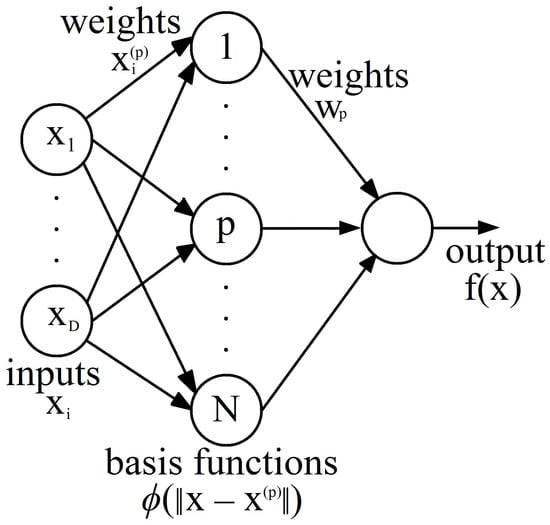
Figure 2.
Radial basis function network under the naïve radial basis function approach.
There are problems with the exact interpolation (naïve radial basis function) approach. First, when the data are noisy, it is not desirable for the network outputs to pass through all data points because the resulting function could be highly oscillatory and would not provide adequate generalization. Second, if the training dataset is very large, the RBFN will not be computationally efficient to evaluate if we employ one basis function for every training data point.
3.3. How Do We Improve Radial Basis Function Networks?
The RBFN can be improved by the following strategies when applying exact interpolation [42]:
- The number of basis functions M must be much smaller than the number of data points N, ();
- Determine the centers of the basic functions using a training algorithm; they should not be defined as training data input vectors;
- The basis functions should have a different width parameter , which could be solved by a training algorithm;
- To compensate for the difference between the mean value of all basis functions and the corresponding mean value of the targets, bias parameters can be used in the linear sum of activations in the output layer.
Notwithstanding the above, proposing the ideal value for M is an open problem. By applying the cross-validation technique discussed in Section 3.1.5, a feasible value M could be obtained by comparing results for a range of different values.
So, how do we find the parameters of an RBFN? The input to hidden “weights” (i.e., radial basis function parameters for ) can be trained using unsupervised learning techniques, such as fixed training data points selected at random and k-means clustering of training data. Supervised learning techniques can also be used, albeit with a higher computational cost. Then, the input-to-hidden “weights” are preserved at a constant while the hidden-to-output “weights” are learned. These weights can be easily found by solving a system of linear equations because this second training stage has only one layer of weights and O linear output activation functions. For more information on RBFN training, please refer to Bishop [29] and Haykin [34].
RBFNs, applied to time series prediction tasks, require inputs of the same form as those used by FFNNs; for instance, we would rearrange our time series data as shown in Table 1 in order to teach an RBFN how to predict one-step-ahead scalar time series values. Recent research on RBFN modeling applied to time series prediction can be found, for instance, in the work of Chang [44], where RBFN models are used to produce short-term forecasts for wind power generation. Other recent examples include the following: in Sermpinis, Theofilatos, Karathanasopoulos, Georgopoulos, and Dunis [45], RBFN-PSO hybrid models are employed for financial time series prediction; Yin, Zou, and Xu [46] use RBFN models to predict tidal waves on Canada’s west coast; Niu and Wang [47] employ gradient-descent-trained RBFNs for financial time series forecasting; Mai, Chung, Wu, and Huang [48] use RBFNs to forecast electric load in office buildings; and Zhu, Cao, and Zhu [49] employ RBFNs to predict traffic flow at some street intersections.
3.4. Recurrent Neural Networks
The main characteristic of a recurrent neural network (RNN) is that it has at least one feedback connection, where the output of the previous step is fed as input to the current step. This recurrent connection system makes RNNs ideal for sequential or time series data, “remembering” past information. Another distinctive feature of an RNN is that each layer shares the same weight parameter. RNNs are not easy to train, but very accurate forecasts for time series can be obtained when trained correctly. There are several RNN architectures; however, they all have the following characteristics in common:
- RNNs contain a subsystem similar to a static FFNN;
- RNNs can take advantage of the nonlinear mapping abilities of an FFNN, with an added memory capacity for past information.
RNN’s learning can be performed by using the gradient descent method, similar to how it is used in the BP algorithm. Specifically, RNNs can be trained by using an algorithm called backpropagation through time (BPTT). BPTT trains the network by computing errors from the output layer to the input layer, but unlike BP, it adds errors at each time step because it shares parameters at each layer.
A basic RNN architecture, called the Elman network [50], has the inputs of the next time step together with its hidden unit activations that feed back on the network. Figure 3a shows the Elman network architecture. It is observed that it is necessary to discretize the time and update the activations step by step. In real neurons, this could correspond to the time scale on which they operate, and for artificial neurons, it could be any time step size related to the prediction to be made. In particular, for time series modeling applications, it seems like a natural choice to make the time-step size in an RNN equal to the time separation between any two consecutive time series values. A delay unit is introduced, which simply delays the signal/activation until the next time step. This delay unit can be regarded as a short-term memory unit. Suppose the vectors and are the inputs and outputs, , , and are the three connection weight matrices, and f and g are the output and hidden unit activation functions of an Elman network; then, the operation of the said RNN can be described as a dynamic system characterized by the pair of nonlinear matrix equations:
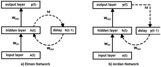
Figure 3.
Two simple types of recurrent neural networks. Each rectangle contains input units, artificial neurons or delay/memory units; their outputs being indicated by vector quantities , , , etc. A solid arrow connecting two rectangles represents the full set of connection weights among all involved units, which are encoded as matrices and . Dashed arrows represent one-to-one connections between involved units; this means (identity matrix) and are diagonal matrices.
In a dynamical system, its state can be represented as a set of values that recapitulates all the information from the past about the system. The hidden unit activations define the state of the dynamical system. Elman networks are useful in modeling chaotic time series, which are more closely related to chaos theory and dynamical systems. For further information on chaotic time series, see Sprott [51]. Some recent applications of Elman networks in time series forecasting can be found in Ardalani-Farsa and Zolfaghari [52], Chandra and Zhang [53], and Zhao, Zhu, Wang, and Liu [54].
Another simple recurrent neural network architecture, similar to an Elman network, is the Jordan network [55]. In this type of recurrent network, it is the output of the network itself that feeds back into the network along with the inputs of the next time step (see Figure 3b). Jordan networks show dynamical properties and are useful for modeling chaotic time series and nonlinear auto regressive moving average (NARMA) processes. Some examples of models based on the Jordan neural network architecture and applied to time series forecasting can be found in Tabuse, Kinouchi, and Hagiwara [56], Song [57] and Song [58].
Another variant of RNN, called nonlinear autoregressive modeling with exogenous inputs (NARX), has feedback connections that enclose several layers of the network, which can be used by including present and lagged values of k exogenous variables , , …, . The full performance of the NARX neural network is obtained using its memory capacity [59].
There are two different architectures of NARX neural network model:
- Open-loop. Also known as the series-parallel architecture, in this NARX variant, the present and past values of and the true past values of the time series are used to predict the future value of the time series .
- Close-loop. Also known as the parallel architecture, in this NARX variant, the present and past values of and the past predicted values of the time series are used to predict the future value of the time series .
3.5. Self-Organizing Maps
Self-organizing maps (SOMs) learn to form their classifications of the training data without external help. To achieve this, in SOMs, it is assumed that membership in each class is determined by input patterns that share similar characteristics and that the network will be able to identify such features in a wide range of input patterns. A particular class of unsupervised systems is based on competitive learning, where output neurons must compete with each other to activate, but under the condition that only one is activated at a time, called a winner-takes-all neuron. To apply this competition, negative feedback pathways must be used, which are lateral inhibitory connections between neurons. As a result, neurons must organize themselves.
The main objective of an SOM is to convert, in a topologically ordered manner, an incoming multidimensional signal into a discrete one- or two-dimensional map. This is like a nonlinear generalization of principal component analysis (PCA).
3.5.1. Essential Characteristics and Training of an SOM
An SOM is organized as follows: we have points in the input space that are mapped to points in the output space. There is a set of points living in the input space, and we suppose that there is a function to assign to points in the output space. In turn, there is another function to assign to each point I in the output space a corresponding point in the input space (see Figure 4).

Figure 4.
Organization of an SOM.
Kohonen networks [60] are a particular and important kind of SOM. The proposed network has a feedforward structure with a single computational layer, where the neurons are arranged in rows and columns. Nodes in the input layer connect to each of the neurons in the computational layer (see Figure 5).
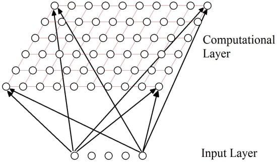
Figure 5.
Kohonen network.
The self-organization process consists of the following components:
- Initialization. At first, the connection weights are set to small random values.
- Competition. For a D dimensionality input space, represents the input patterns and represents the connection weights between the input units and the neuron j in the computational layer; , where N is the total number of neurons. The difference between for each neuron can be calculated as the Euclidean distance squared, which will represent the discriminant function .The neuron with the lowest discriminant function is declared the winner-takes-all neuron. Competition between neurons allows mapping the continuous input space to the discrete output space.
- Cooperation. In neurobiological studies, it was observed that, within a set of excited neurons, there can be lateral interaction. When a neuron is activated, the neurons in its surroundings tend to become more excited than those further away. A similar topological neighborhood that decays with distance exists for neurons in an SOM. Let be the lateral distance between any pair of neurons i and j, then defines our topological neighborhood, where is the index of the winner-takes-all neuron. A special quality of the SOM is that the size of the neighborhood should decrease over time. An exponential reduction is a commonly used time dependence: .
- Adaptation. SOM has an adaptive (learning) process through which the feature map between inputs and outputs is formed through the self-organization of the latter. Due to the topographic neighborhood, when the weights of the winner-takes-all neuron are updated, the weights of its neighbors are also updated, although to a lesser extent. To update the weight, we define , in which we have a time-dependent learning rate t. These updates are applied to all training patterns for various periods. The goal of each learning weight update is to move the weight vectors of the winner-takes-all neuron and its neighbors closer to the input vector .
When the SOM training algorithm has converged, important statistical properties of the feature map are displayed. As shown in Figure 4, the set of weight vectors in the output space integrates the feature map , which provides an approximation to the input space. Derived from the above, represents the statistical variations in the input distribution: the largest domains of the output space are allocated to sample training vectors with high probability of occurrence, which are drawn from the regions in the input space; the opposite is the case for training vectors with low probability. In other words, a properly trained self-organizing map is able to choose the best features to approximate the underlying distribution of the input space. For further details on SOM statistical properties, please refer to Haykin [34].
3.5.2. Application of Self-Organizing Maps to Time Series Forecasting
If SOMs are mainly employed to solve unsupervised classification problems, how can they be applied to time series forecasting tasks, which in essence are, as we saw in Section 2.2, function approximation (regression) problems? A simple approach to the univariate time series case is as follows: as training examples for our SOM model, we can use vectors of the form , where the first component corresponds to the one-step-ahead target output in our basic FFNN model discussed in Section 3.1. The rest of the components in correspond to the autoregressive inputs also employed by our FFNN model. Thus, any single row in Table 1, which corresponds to a training example for FFNN models, also serves as a training example for SOM models. The computational layer in our SOM model for univariate time series consists of a one-dimensional lattice of neurons. When forecasting, our SOM model utilizes all of the components from input vector , except for the first, in a competition process among all neurons in the computational layer, just as described in Section 3.5.1. The winning neuron determines our one-step-ahead forecast value by simply extracting the first component from weight vector associated to winning neuron , i.e., . Thus, the number of neurons in the computational layer determines how many possible discrete values can assume our one-step-ahead forecast value . One disadvantage to this simple approach is the large prediction error due to the step-like output of our SOM model trying to approximate a “smooth” time series. SOMs may require too many neurons if we want to reduce their associated prediction error. This alternative, however, would be accompanied by a prohibitively high computational cost. A more sensible solution to this problem would be using RBFNs in conjunction with SOMs: first, we train a univariate time series SOM model just as described above; then, the resulting SOM weights , which define mapping , are used to directly build an RBFN with N Gaussian basis functions and one output unit. SOM weights would be used as RBFN hidden-to-output weights, while the remaining components in vector would play the role of the RBF center for the jth hidden unit. No further RBFN training is required, although we still need to determine the parameters for each radial basis function in the network; refer to Section 3.2 for more details on RBFNs. Thus, a reduction in prediction error is achieved, at least in places where there are not extreme values in the time series. In these particular locations where extreme values occur, prediction errors are still high for both SOM and SOM–RBFN models. For more details, see Barreto [61], where a comprehensive survey on SOMs applied to time series prediction can also be found. Relatively recent work on model refinements based on the classical SOM and applied to time series prediction can be found in Burguillo [62] and Valero, Aparicio, Senabre, Ortiz, Sancho, and Gabaldon [63]. In Section 4.4, we summarize the work of Simon, Lendasse, Cottrell, Fort, Verleysen, et al. [64], where a double SOM model is proposed to generate long-term time series trend predictions.
3.5.3. Comparison between FFNN and SOM Models Applied to Time Series Prediction
An SOM-based model adapted to time series prediction basically performs local function approximation, i.e., acts on localized regions of the input space. On the other hand, FFNNs are global models, making use of highly distributed representations of the input space. This contrast between global and local models implies that FFNN weights are difficult to interpret in the context of time series modeling. Essentially, FFNNs are black boxes that produce forecasts in response to certain stimuli. The components of a weight vector associated to each neuron in an SOM model fitted to a univariate time series can have a clearer meaning to the user, given the local nature of the model. Specifically, they can be viewed as the mean values for lagged versions of response variable y when we expect a one-step-ahead future value close to the first component on such a weight vector [61].
3.5.4. SOM Models Combined with Autoregressive Models
Another possible approach involving the application of SOM models to time series prediction tasks is a direct extension of the procedure described in Section 3.5.2. We can build a hybrid two-stage predictor based on SOM and autoregressive (AR) models. In the first stage, we train an SOM model so as to produce discrete one-step-ahead time series forecasts.This SOM model is then employed to split the available set of training examples into N clusters, one for each SOM neuron, by simply presenting training example to trained SOM and assigning a cluster label to based on the winning neuron. In the second stage, a local linear AR model is fitted to each cluster defined in the first stage. Now, this fully trained hybrid model can be employed to produce a one-step-ahead forecast for any future input : first, we determine to which cluster belongs, by using our trained first-stage SOM model; then, we use the corresponding AR model to produce the desired forecast. This basic approach is similar in spirit to local function linearization (it seems like a sensible strategy to assume that, locally, a real continuous function can be reasonably approximated by a simpler linear function) and can be extended in many ways; for instance, FFNN (or RBFN, or even RNN) ensembles could replace local AR models in the second stage. Although, this would result in a more complex model, requiring extensive computational resources for its construction. AR parameters can be quickly computed, although statistical training on the modeler’s side is required (specifically, the modeler must be familiarized with the Box–Jenkins statistical technique). This SOM–AR approach will work well if each data cluster contains enough consecutive time series observations to adequately train an AR model; otherwise, an ANN alternative for the second stage would be preferable. If all goes well, two-stage SOM–AR models will enable users to make plausible statistical inferences about the relative importance of lagged time series values at a local level. Confidence intervals can additionally be computed for each one-step-ahead forecast produced by the SOM–AR model, giving a statistical quantification of forecast uncertainty. Yadav and Srinivasan [65] propose a specific SOM–AR model implementation for predicting electricity demand in Britain and Wales, while Dablemont, Simon, Lendasse, Ruttiens, Blayo, and Verleysen [66] combine an SOM clustering model with local RBFNs to forecast financial data; Cherif, Cardot, and Boné [67] propose an SOM–RNN model to forecast chaotic time series, and Nourani, Baghanam, Adamowski, and Gebremichael [68] propose a sophisticated SOM–FFNN model to forecast rainfall on multi-step-ahead time scales using precipitation satellite data.
3.6. BP Problems in the Context of Time Series Modeling
We have seen in Section 3.1.2 that BP training presents several challenges that must be overcome: over-fitting, convergence to a local minimum, and convergence problems slow convergence speed ( must be small to improve BP convergence properties at the expense of BP processing speed).
3.6.1. Vanishing and Exploding Gradient Problems
One of the main problems encountered when training recurrent neural networks or deep neural networks (FFNNs with many hidden layers) with BP is the vanishing gradient problem. When the gradients become very small relative to the parameters, it can cause the weights in the initial layers not to change noticeably; this is known as the vanishing gradient problem [69]. This problem is commonly attributed to the architecture of the neural network, certain activation functions (sigmoid or hyperbolic tangent), and small initial values of the weights. The exploding gradient problem appears when the weights are greater than 1 and the gradient continues to increase, causing the gradient descent to diverge. Unlike the vanishing gradient problem, the exploding gradient problem is directly related to the weights in the neural network [69].
For instance, a generic recurrent network has hidden states , inputs , and outputs . Let it be parametrized by , so that the system evolves as
Often, the output is a function of , as some . The vanishing gradient problem already presents itself clearly when , so we simplify our notation to the special case with
Now, take its differential:
Training the network requires us to define a loss function to be minimized. Let it be , then minimizing it by gradient descent gives
where is the learning rate. The vanishing/exploding gradient problem appears because there are repeated multiplications of the form
Specifically, the vanishing gradient problem arises when the neural network adds multiple layers with activation functions whose gradients approach zero. Since each layer contributes to the product of the activation functions and the layer weights, if the number of layers increases, the product quickly turns small [70].
The explosive gradient problem arises when the network weights are multiplied by the activation functions, and as a result, we have a product with values greater than one, causing the values of the gradients to be large [70].
3.6.2. Alternatives to the BP Problems
Attempts have been made to overcome these issues in the context of time series forecasting. See, for example, Hu, Wu, Chen, and Dou [71] and Nunnari [72]. Below is a brief outline of the main alternatives.
Batch normalization. Ioffe and Szegedy [73] described an internal covariate shift as the effect of inputs with a corresponding distribution in each layer of a neural network, which is caused by the randomness that exists in the initialization of parameters and in the input data during the training process. They proposed to address the problem by normalizing the layer inputs, recentering and rescaling them, and applying the normalization to each training mini-batch. Batch normalization relaxes the care of parameter initialization, allows the application of much higher learning rates, and, in certain cases, eliminates the need for dropout to mitigate overfitting. Although batch normalization has been proposed to handle gradient explosion or vanishing problems, recently, Yang, Pennington, Rao, Sohl-Dickstein, and Schoenholz [74] showed that, at the initialization time, a deep batch norm network suffers from gradient explosion.
Gradient clipping. In 2013, Pascanu, Mikolov, and Bengio [70] assumed that a cliff-like structure appears on the error surface when gradients explode, and as a solution, they proposed clipping the norm of the exploded gradients. Furthermore, to solve the vanishing gradient problem, they use a regularization term to force the Jacobian matrices to preserve the norm only in relevant directions, keeping the error signal alive while it travels backwards in time.
Backpropagation through time (BPTT). This famous technique was proposed by Werbos [75] in 1990. If the computational graph of an RNN is expanded (unrolled RNN), it is basically an FFNN with the innovative characteristic that, throughout the unrolled RNN, the same parameters are repeated and these appear in each period. Then, the chain rule can be applied to propagate the gradients backward through the unrolled RNN, as would be performed in any FFNN. It should be considered that, in this unrolled RNN, for each parameter, the gradient with respect to itself must be added at all places where the parameter occurs. In summary, BPTT can be explained as using BP to RNN on sequential data, e.g., a time series [75].
The BPTT algorithm can be described as follows:
- Introduce a time-step sequence of input and output pairs to the network.
- Unroll the network.
- For each time step, calculate and accumulate errors.
- Roll-up the network.
- Update weights.
- Repeat.
Long short-term memory (LSTM). In 1997, Hochreiter and Schmidhuber [76] introduced an RNN along with an appropriate gradient-based learning algorithm. Its goal is to introduce a short-term memory for RNN that can last for thousands of time steps, that is, a “long short-term memory”. The main feature of LSTM is its memory cell made up of three “gates”: the input gate, output gate, and forget gate [77]. The flow of information is regulated by gates inside and outside the cell. First, the forget gate assigns a previous state a value between 0 and 1, compared to a current input. Then, it chooses what information to keep from a previous state. A value of 0 means deleting the information, and a value of 1 means keeping it. By applying the same system as the forget gate, the gateway determines the new information that will be stored in the current state. Finally, the output gate controls which pieces of information in the current state are generated by considering the previous and current states and assigning a value from 0 to 1 to the information. The LSTM network maintains useful long-term dependencies, generating relevant information about the current state.
The goal of LSTM is to create an additional module in an ANN that can learn when to forget irrelevant information and when to remember relevant information [77]. Calin [78] shows that RNNs using LSTM diminish the vanishing gradient problem but do not solve the exploding gradient problem.
Reducing complexity. The vanishing gradient problem can be mitigated by reducing the complexity of the ANN. By reducing the number of layers and/or the number of neurons in each layer, a reduction in the complexity of the network can be achieved, affecting the tunability of the model. Therefore, finding a balance between model complexity and gradient flow is critical to creating successful ANNs in deep learning.
Evolutionary algorithms. Alternatively, it is also possible to employ evolutionary algorithms instead of BP for ANN training purposes [79]. For instance, Jha, Thulasiraman, and Thulasiram [80] and Adhikari, Agrawal, and Kant [81] employ particle swarm optimization (PSO) to train ANN models applied to time series modeling; Awan, Aslam, Khan, and Saeed [82] compare short-term forecast performances for FFNN models trained with genetic algorithm (GA), artificial bee colony (ABC), and PSO by using electric load data; Giovanis [83] combines FFNN and GA for predicting economic time series data.
Statistical techniques ANNs can also be trained using probabilistic techniques such as the Bayesian learning framework. This training technique offers some relevant advantages: no over-fitting occurs, it provides automatic regularization, and forecast uncertainty can be estimated [29]. Some recent applications using this approach in the context of time series forecasting can be found, for example, in Skabar [84], Blonbou [85], van Hinsbergen, Hegyi, van Lint, and van Zuylen [86], and Kocadağlı and Aşıkgil [87]. Another possible alternative is to train an ANN with BP or some other optimization technique and then build a hybrid ANN–ARIMA model; see, for example, Zhang [88], Guo and Deng [89], Otok, Lusia, Faulina, Kuswanto, et al. [90], and Viviani, Di Persio, and Ehrhardt [91].
4. Brief Literature Survey on ANNs Applied to Time Series Modeling
In this section, we discuss, analyze, and summarize a small sample of recently published research articles. In our opinion, these articles are representative of the state of the art and provide useful information that can be used as a starting point for future research. The choice of articles surveyed in this section is based mainly on the architectures outlined previously in Section 3. In Section 4.1, we study some time series forecasting techniques [92,93], which combine feedforward neural network models with particle swarm optimization. The basic idea here is to show how to combine these techniques to produce new hybrid models and how to design experiments in which we compare several time series prediction models. Section 4.2 explores the work of Crone, Guajardo, and Weber [94] on how to assess the ability of support vector regression and feedforward neural network models to predict basic trends and seasonal patterns found in economic time series of monthly frequency. Section 4.3 highlights useful hints suggested by Moody [95] on how to construct ANN models for predicting short-term behavior in macroeconomic indicators. Section 4.4 summarizes the work found in Simon, Lendasse, Cottrell, Fort, Verleysen, et al. [64], which instructs on how to build a model based on a double application of the self-organizing map to predict medium- to long-term time series trends, focusing on the empirical distribution of several forecasts’ paths produced by the same double SOM model. Section 4.5 and Section 4.6 summarize the works of Zimmermann, Tietz, and Grothmann [96] and Lukoševičius [97], respectively. Both works contain valuable hints and techniques to build recurrent neural network models aimed at predicting temporal data, possibly coming from an underlying dynamical system. Zimmermann, Tietz, and Grothmann [96] focus on a more traditional approach, using back propagation through time as a training algorithm but employing a novel graphical notation to represent recurrent neural network architectures. Lukoševičius [97] focuses on the echo state network approach, which relies more on numerical linear algebra for training purposes. In Section 4.2–Section 4.6, we replicated, from the respective surveyed articles, important comments that correspond to theoretical concepts, hints, and relevant bibliographic references, as we believe this is the best way to convey and emphasize them. Our intention is to construct useful, short, and clear summaries that will hopefully save some time for readers interested in gaining a full understanding of similar articles to the ones we are surveying here.
4.1. Combining Feedforward Neural Networks and Particle Swarm Optimization for Time Series Forecasting
As we mentioned already briefly in Section 3.6, it is possible to train ANN models via evolutionary algorithms. The objective of evolutionary algorithms is to discover global solutions that are optimal and low cost. Evolutionary algorithms are usually based on various agents, such as chromosomes, particles, bees, ants, etc., searching iteratively to discover the global optimum or the local optimum (population-based algorithms) [36]. In 1975, Holland [98] introduced the genetic algorithm (GA), which is considered the first evolutionary algorithm. As with any evolutionary algorithm, the GA is based on a metaphor from the theory of evolution. In the field of evolutionary computing, good solutions to a problem can be seen as individuals well-adapted to their environment. Although the GA has had many applications, it has been surpassed by other evolutionary algorithms, such as the PSO algorithm [99].
Today, due to its simplicity and ability to be used in a wide range of applications, the PSO algorithm has become one of the most well-known swarm intelligence algorithms [100]. Eberhart and Kennedy performed the first experiment using PSO to train ANN weights instead of using the more traditional backpropagation algorithm [101]. Several approaches have been proposed to apply PSO in ANN, such as the works published by Eberhart and Shi [102], Eberhart and Shi [103], and Yu, Wang, and Xi [104]. In this section, we explore in a little more detail some possible ways we can pair an ANN model with the PSO algorithm to produce time series forecasts, but first, we will briefly describe how PSO works.
In the words of its creators…
PSO is an optimization algorithm inspired by the motion of a bird flock; any member of the flock is called a “particle”.(Kennedy and Eberhart [101], 1995)
In the PSO algorithm, a particle moves through a real-valued dimensionality search space D, guided by three attributes at each time (iteration) t: position , velocity , and memory . In the beginning, the position of the particle is generated by a random variable with a uniform distribution, delimited in each dimension by the search space ; thereby, its best visited position is set as equal to its initial position , with an initial velocity . After the first iteration, the attribute remembers the best position visited by the particle based on an objective function f; the other two attributes, and , are updated according to Equations (15) and (16), respectively.
The best of all the best particle positions is called the global best . In each iteration of the algorithm, the swarm is inspected to update the best member. Whenever a member is found to improve the objective function of the current leader, that member becomes the new global best [105].
The objective of the PSO algorithm is to minimize function ; i.e., find such that for all in the search space.
In PSO, variation (diversity) comes from two sources. The first is the difference between the current position of particle and its memory . The second is the current position of particle and the global best (see Equation (15)).
Equation (15) reflects the three main elements of the PSO algorithm: the inertia path, local interaction, and neighborhood influence [106]. The inertial path is the previous velocity , where is the inertial weight. The local interaction is called the cognitive component , with as the cognitive coefficient. The last term is called the social component and represents the neighborhood influence , where is the social coefficient. is a random variable with a uniform distribution [105]. In [107], Clerc and Kennedy proposed a set of standard parameter values for PSO stability and convergence: , , and .
A leader can be global to the entire swarm or local to a certain neighborhood of a swarm. In the latter case, there will be as many local leaders as there are neighborhoods, resulting in more attractors scattered throughout the search space. The use of multiple neighborhoods is useful to combat the premature convergence problem of the PSO algorithm [105].
4.1.1. Particle Swarm Optimization for Artificial Neural Networks
In Algorithm 1, the basic PSO algorithm proposed by Kennedy and Eberhart [101] is presented.
| Algorithm 1 Basic particle swarm optimization (PSO) algorithm |
| for each particle in the swarm do |
| initialize particle’s position: uniform random vector in |
| initialize particle’s best-known position: |
| if then |
| update swarm’s best-known position: |
| end if |
| initialize particle’s velocity: uniform random vector in |
| end for |
| repeat |
| for each particle in the swarm do |
| for each dimension do |
| pick random numbers |
| update particle’s velocity: |
| end for |
| update particle’s position: |
| if then |
| update particle’s best-known position: |
| if then |
| update swarm’s best-known position: |
| end if |
| end if |
| end for |
| until a termination criterion is met |
| Now, holds the best found solution |
The basic PSO algorithm shown in Algorithm 1 can be applied to ANNs as a multilayer perceptron, where each particle’s position represents the set of weights and biases of the ANN for the current iteration. Each particle moves in the weighting space trying to minimize the learning error during the training phase, and also maintains the historically best position in memory along its exploration path. When the particle changes position, it is analogous to updating the weights of the ANN controller to reduce the tracking error [108]. The termination criterion can be defined as the scope of a predefined MSE value condition [109]. Finally, the best position reached by the swarm can be expressed as the optimal solution for the ANN.
Now let us take a look at some FFNN–PSO time series models proposed in the literature. Adhikari, Agrawal, and Kant [81] assess the effectiveness of FFNN and Elman networks when trained with the PSO algorithm for the prediction of univariate seasonal time series. In this context, a PSO particle moves in the search space defined by the weights of the ANN model to be trained, while the PSO cost function is the same cost function employed in backpropagation; thus, we could say that a PSO particle is structurally identical to an ANN.
de M. Neto, Petry, Aranildo, and Ferreira [92] take a slightly different approach: they propose a basic PSO optimizer in which each particle is a single hidden layer FFNN designed to produce one-step-ahead forecasts for univariate time series, plus some extra meta-parameters. The search space for their proposed hybrid system consists of the following discrete and continuous variables:
- Relevant time lags for autoregressive inputs (the total number of relevant time lags defines the FFNN’s input dimension d);
- Number q of hidden units in the FFNN;
- Training algorithm employed: 1. Levenberg–Marquardt [110], 2. RPROP [111], 3. scaled conjugate gradient [112], or 4. one-step secant [113], all refinements of the basic BP algorithm;
- Variant of FFNN architecture employed: 1. An FFNN architecture identical to the one outlined in Section 3.1, with a linear output unit, 2. an FFNN with structural modifications proposed by Leung, Lam, Ling, and Tam [114], or 3. the same FFNN architecture as in 1, but with a sigmoidal output unit;
- Initial FFNN weights and meta-parameter configuration.
PSO individuals in this combined method are evaluated by a proposed fitness function, which is directly proportional to a metric measuring the degree of synchronization between time series movements in forecasts and corresponding time series movements in validation data. The proposed fitness function is also inversely proportional to the sum of several regression error metrics, among them, mean squared error (MSE) and Theil’s U statistic.
We now summarize, in the next few lines, the experiments conducted by de M. Neto, Petry, Aranildo, and Ferreira [92], their observations, and their conclusions. All investigated time series were normalized to lie within the interval [0,1] and were divided into three sets: the training set with 50% of the data, the validation set with 25% of the data, and the test set with 25% of the data. Ten particles were used in the PSO algorithm, with 1000 iterations. The standard PSO optimization routine was employed to find the minimum in the parameter space; in this way, an optimal FFNN model is found for each time series. This optimal FFNN was then compared (via the same regression error metrics employed in the proposed fitness function) against a random walk model and a standalone FFNN model trained with the Levenberg–Marquardt algorithm.
Benchmarking data used in the experiments consist of two natural phenomena time series (daily starshine measures and yearly sunspot measures) and four financial time series of daily frequency (Dow Jones Industrial Average Index (DJIA), National Association of Securities Dealers Automated Quotation Index (NASDAQ), Petrobras Stock Values, and Dollar-Real Exchange Rate). From these experiments, it was observed that the proposed model behaved better than the random walk model, the heads or tails experiment, and the standalone FFNN model for the two time series of natural phenomena that were analyzed. Nevertheless, for the four financial time series that were forecast, the proposed model displayed behavior similar to both a random walk model and a heads or tails experiment and behaved slightly better than the standalone FFNN model. It was also observed by the authors that predictions for all analyzed financial series are dislocated one-step-ahead with respect to the original values, noting that this observed behavior is consistent with the work of Sitte and Sitte [115] and de Araujo, Madeiro, de Sousa, Pessoa, and Ferreira [116], which have shown that the forecast of financial time series denotes a distinctive one-step shift concerning the original data.
Finally, de M. Neto, Petry, Aranildo, and Ferreira [92] claim that this behavior can be corrected by a phase prediction adjustment, and conclude that their proposed method is a valid option for predicting financial time series values, obtaining satisfactory forecasting results with an admissible computational cost.
Now let us take a look at a similar but more refined approach. Simplified swarm optimization (SSO) [117] is a refinement of PSO, which, of course, can also be employed for adjusting ANN weights. SSO is a swarm intelligence method that also belongs to the evolutionary computation methods. SSO’s updating mechanism for particle position is much simpler than that of PSO.
In turn, parameter-free improved simplified swarm optimization [93], or ISSO for short, is a refinement of SSO; ISSO treats SSO’s tunable meta-parameters as variables in the search space where particles move. The idea here is to reduce human intervention during the optimization process, i.e., minimize the need for manual tuning of meta-parameters. In Yeh [93], ISSO is employed for adjusting ANN weights. ISSO uses three different position updating mechanisms: one for updating ANN weights, a second one for updating SSO meta-parameters, and a third one for updating the whole position of a particle if its associated fitness value shows no improvement after several iterations in the process. Yeh [93] conducted a couple of experiments to compare ISSO against five other ANN training methods: BP, GA [118], basic PSO, a PSO variant called cooperative random learning PSO [119], and regular SSO.
- Experiment number 1 tests all six training algorithms on a special ANN architecture called single multiplicative neuron (SMN), which is similar to an FFNN but consists of an input layer and an output layer with a single processing unit (this single neuron has a logistic activation function but multiplies its inputs instead of adding them; additionally, there is a bias for each input node, in contrast to FFNNs, which contain just one bias in the input layer).
- Experiment number 2 also tests all six training algorithms, but this time on a regular FFNN with one to six hidden neurons.
Time series employed in this experiment were as follows: Mackey–Glass chaotic time series [120], Box–Jenkins gas furnace [121], EEG data [122], laser-generated data, and computer-generated data [123]. All time series values were transformed to be in the interval in order to avoid saturation of neural activations and improve convergence of training algorithms. In both experiments, each model was trained 50 times for each time series; 30 particles/chromosomes were employed in each training session. The training algorithms were allowed to run for 1000 generations. The measures used to compare the results were the mean square error (MSE), standard deviation of MSE test errors, and CPU processing time. According to the author, the results from both experiments showed that ISSO outperformed the other five training algorithms, with the exception of BP, which performed better in experiment 1 when forecasting the laser-generated data. Additionally, the FFNN models produced forecasts that were more accurate than the ones generated by the SMN model.
4.1.2. Particle Swarm Optimization Convergence
To prevent the basic gradient descent method (applied in BP) from being caught at the local minimum, we can apply PSO to ANN to optimize the values of the weights’ and biases’ parameters. Although the PSO algorithm has been shown to perform well, researchers have not adequately explained how it works. In 2003, Gudise and Venayagamoorthy [124] made a comparison of the BP and PSO algorithms, analyzing the computational requirements when used in ANN training. They concluded that when the PSO algorithm is used, the FFNN weights converge faster, outperforming the BP algorithm. Liu, Ding, Li, and Yang [125] used a BP–ANN based on the PSO algorithm (PSO–BP). They demonstrated that their proposed PSO–BP algorithm outperforms a BP trained based on the Levenberg–Marquardt (LM) algorithm for training ANNs. Ince, Kiranyaz, and Gabbouj [126] proposed to find not only the weights of an FFNN but also the optimal architecture of the network, applying the MD–PSO algorithm: a modified version of the PSO. Their approach was to find the optimal number of dimensions for the search space simultaneously searching for the optimal solution in that proposed search space. The MD–PSO algorithm chose the global optimal solution among the optimal solutions found for each dimension. Several works have proposed variants of PSO against BP to optimize ANN [127,128,129,130]. However, like other evolutionary algorithms, PSO has some disadvantages, such as an imbalance between exploration and exploitation, sensitivity to parameters, and premature convergence [36]. These problems have been mostly solved by including new parameters, modifying the algorithm with additional operators, or creating hybrid versions with other algorithms [131]. Since its original version in 1995, the PSO algorithm has been expanded to solve a variety of different problems [100]. Multimodal, constrained, and multiobjective optimization problems are some of the most prominent applications that have been addressed with the PSO algorithm [132].
But the question is, why does PSO outperform BP? The study of PSO to optimize ANN has had very good results, but there is no in-depth research on theoretical aspects. Nevertheless, there are works that have tried to explain the PSO convergence. In 2002, Clerc and Kennedy [107] analyzed the full stochastic system of a deterministic version of PSO to supply knowledge about its search mechanism. They proposed reducing the particle velocity formula (Equation (15)) by redefining it as follows:
where and . This is algebraically identical to the standard two-term form [133]. The analysis begins by removing all coverings from a particle, for example, a population of a one-dimensional deterministic particle, with a constant P and a constant . Kennedy [133] observed that the value of the parameter controls the trajectory of the particle and recognized that the explosion of the system depended on randomness. In [134], the authors analyzed the same system and concluded that the particle trajectories follow periodic sinusoidal waves. In their work, Clerc and Kennedy [107] analyzed the movement in discrete time of the PSO, advancing to its visualization in continuous time. These analyses lead to a proposal of controlling the convergence tendencies of the system through a set of coefficients, resulting in a generalized model of the algorithm. When they re-introduced randomness into the PSO with constriction coefficients, the deleterious effects of randomness were seen to be controlled. As a result of this study, the velocity equation changes to
where is the constriction coefficient calculated as
with and . The constant controls the rate of convergence. For , faster convergence to a stable point is achieved, and for , slow convergence to a stable point is obtained [107].
In 2010, van den Bergh and Engelbrecht [135] formally demonstrated that the original PSO is not a local or global optimizer. They identified an imperfection in PSO and addressed it in their approach called guaranteed convergence PSO (GCPSO). The goal of the GCPSO is to update only the speed of the best particle in the swarm () to
Equation (21) has three terms: the first term introduces a direct relationship with the current global best position, the second term conveys the inertia of the global best particle, and the third term shows a point of a uniform distribution in a hypercube with side lengths ; is strictly greater than zero. The authors indicate that their proposal ensures that the best global particle never stops moving completely. van den Bergh and Engelbrecht [135] showed that the GCPSO is a local optimizer.
In 2012, Kan and Jihong [136] demonstrated the existence and uniqueness of the convergence position in PSO, using the theorem of Banach space and the contraction mapping principle. They gave the parameter condition that influences the stability of PSO and showed that, if the parameter satisfies this condition, the probability that the particle swarm optimization converges to the best position is one. In 2018, Qian and Li [137] proposed an improved PSO (IPSO) algorithm according to the following strategy. They introduced a Gaussian perturbation in the position to guarantee that IPSO converges to the -optimum solution with probability one for any . Also in 2018, Xu and Yu [138] defined the swarm state sequence and examined its Markov properties according to the theory of PSO. Subsequently, from the evolutionary sequence of the particle swarm with the best fitness value, the authors derived a supermartingale. Based on this result, the authors applied the supermartingale convergence theorem to analyze the convergence of the PSO. The results show that PSO reaches the global optimum in probability. Recently, Huang, Qiu, and Riedl [139] established PSO convergence to a global minimizer based on continuous-time modeling for a non-convex and non-smooth objective function of particle dynamics through a system of stochastic differential equations.
In summary, there are several works that prove the convergence of PSO. However, it may be interesting to carry out a study of the convergence properties of PSO to optimize ANNs.
4.2. A Study on the Ability of Support Vector Regression and Feedforward Neural Networks to Forecast Basic Time Series Patterns
According to Crone, Guajardo, and Weber [94], “Support Vector Regression (SVR) and Feed Forward Neural Networks (FFNNs) have found increasing consideration in forecasting theory, leading to successful applications in time series forecasting for various domains, often outperforming conventional statistical approaches of ARIMA -or exponential smoothing- methods. Despite their theoretical and practical capabilities, FFNN and SVR models are not established forecasting methods. Substantial theoretical criticism on FFNNs has raised skepticism regarding their ability to forecast even simple time series patterns of seasonality or trends without prior data preprocessing [140]”. In their study, Crone, Guajardo, and Weber [94] propose an empirical comparison between three different models:
- FFNNs;
- SVR models using a radial basis function (RBF) kernel;
- SVR models using a linear function kernel.
This study reflects, for the considered models, their ability to learn and forecast fundamental time series patterns relevant to empirical forecasting tasks. Next, SVR models are briefly described (description based on text in Crone, Guajardo, and Weber [94]).
Support vector regression. For their experiment, Crone, Guajardo, and Weber [94] employed the common support vector regression (SVR) algorithm described in [141], which applies an -insensitive loss function for predictive regression problems. Let , where and are the training data points available to build a regression model. A transformation function on the initial input space is applied to map the original data points to a higher dimensional feature space . A linear model is constructed in in correspondence with the nonlinear model of the original space:
is the inner product between and . The insensitive loss function allows you to fit a function that is as flat as possible and has a maximum deviation for the current training data. This means that we are looking for a small weight vector . To solve this problem, the authors introduce slack variables to allow error levels higher than , obtaining the following:
The construction of the objective function considers two key aspects: the precision in the training set and the generalization capacity, which lead to the principle of minimization of structural risk. The balance between generalization ability and accuracy is measured by C in the training data, and the degree of error tolerance is defined by . It is convenient to represent the problem in its dual form for its resolution, so a Lagrange function is constructed, from which it can be shown that once the saddle point conditions are applied, the following solution is reached:
Here, and are the dual variables, and the expression represents the inner product between and , which is known as the kernel function. It is possible to achieve a solution to the original regression problem, starting from the existence of the kernel function, leaving aside the transformation applied to the data. For more information on SVR models, please consult Drucker, Burges, Kaufman, Smola, and Vapnik [13].
Experiments and results. Crone, Guajardo, and Weber [94] employed a set of five artificial time series in their experiments (see Figure 6):
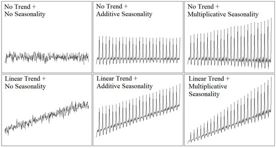
Figure 6.
Some basic time series patterns according to Pegel and Gardner’s classification. All of these patterns (except for the no trend + multiplicative seasonality) were generated artificially in the experiment of Crone, Guajardo, and Weber [94].
- Stationarytime series (constant level);
- Stationary time series with additive seasonality;
- Linear trend;
- Linear trend with additive seasonality;
- Linear trend with multiplicative seasonality.
These artificial data emulate the behavior of monthly retail sales and are taken from Pegel and Gardner’s original classification. All artificial series contain additive Gaussian white noise, with . Each time series consists of 228 observations. A lag structure of 13 previous observations was established to produce one-step-ahead forecasts (this number of lags should be adequate to capture seasonal patterns present in monthly time series). Thus, 215 examples are available to construct FFNN and SVR models. From these available examples, the first 119 were reserved for model training, the next 48 for model validation, and the last 48 for model testing.
All models were constructed by using training and validation data only, retaining all information in the test suite to ensure valid predicted event testing. To avoid saturation effects, a linear scale in an interval was applied in the data transformation, using minimum and maximum values only from the training and validation data. In order to evaluate model performance, mean squared error (MSE), mean absolute error (MAE), and root mean squared error (RMSE) metrics were employed to measure test errors. MAE was employed to fine-tune model meta-parameters (C and for SVR–linear; C, , and for SVR–RBF; number of hidden nodes and type of activation function for FFNN hidden nodes; available options were sigmoid or hyperbolic tangent). After the construction of all models and test error measuring, Crone, Guajardo, and Weber [94] arrived at the following conclusions:
- The performance of FFNNs and SVRs with linear kernel is similar; they both robustly forecast time series patterns without preprocessing;
- Considering the results obtained in the three error measures of MAE, MSE, and RMSE, the FFNNs outperform the SVR models in the time series forecast of the different patterns tested;
- The results obtained indicate that FFNNs seem to be able to extrapolate seasonal trends and patterns accurately and without preprocessing.
4.3. Forecasting the Economy with Artificial Neural Networks
It is of great interest to economists to forecast the “business cycle”. It affects the economic system of any country due to its fluctuations that impact macroeconomic indicators, such as interest rates, housing demand, occupancy rate, demand for manufactured goods, etc. The economic cycle also affects relevant sociopolitical factors, such as the result of a country’s presidential elections. Economists use the Gross Domestic Product (GDP) and the Index of Industrial Production (IIP) to track the business cycle [95]. In this contribution, Moody [95] stresses the reasons why macroeconomic modeling and forecasting are challenging tasks:
- Macroeconomics is a non-experimental science. It is a complicated task to observe the behavior of an economy as a whole, and the possibility of carrying out controlled experiments is very remote;
- Lack of a priori models. It is not possible to carry out controlled studies on the effects of the influence that qualitative (non-quantifiable) variables have on economic activity, due to the complexities of the economic system;
- Noise present in data. This is due to two main causes: the way in which information is collected and the number of unobserved (non-measurable) variables in economics. The presence of noise in short time series makes it difficult to control the variance of the model, requiring highly complex models to predict this type of phenomena;
- Nonlinearity. Due to high levels of noise and limited data, neural network models do not capture the nonlinear characteristics of macroeconomic series.
In our view, the perceived difficulty in modeling macroeconomic data’s nonlinear features is one of the main reasons why many practitioners still use traditional statistical linear techniques to model macroeconomic data (for instance, several official statistics agencies around the world rely on X13ARIMA-SEATS [142] to generate ARIMA-based forecasts for macroeconomic time series). On the other hand, there is a growing group of researchers who feel that it is worth continuing with investigations of efficient ANN models that take into account nonlinear features of macroeconomic data since ANNs are capable of achieving universal function approximation. For example, Kiani [143] applied nonlinear regime change models and artificial neural networks to anticipate the impact of monetary policy shocks on GDP.
Neural Network Challenges in Economy
Moody [95] categorizes several heuristics for ANN model selection and construction, aimed at minimizing expected prediction error. Considered categories are the following:
Meta-parameter selection. Adjusting the regularization parameter can compensate for bias and variance in the forecast, while varying the number of input nodes can compensate for noise and non-stationarity [144].
Input variable selection and pruning. The appropriate selection of input variables is essential for the solution of any prediction problem. The set of variables selected must be representative and provide the greatest possible information with the least amount of them [145,146,147].
Model selection and pruning. Selecting the right size and appropriate network architecture is a key element in controlling the balance between bias and variance. The above involves eliminating unnecessary weights or nodes, choosing the number of hidden units, selecting a connectivity structure, etc. [148,149,150,151].
Better regularizers. Regularization of ANNs reduces model variance and minimizes prediction risk, improving model generalization [152,153].
Committee forecasts. Several economic researchers have made forecasts using a forecasting committee. The approach consists of averaging (weighted or unweighted) the predictions of an ensemble of models [144].
Model interpretation and visualization. In general, great importance is placed on obtaining accurate forecasts, leaving aside the understanding of the factors that influence these forecasts. Sensitivity analysis (SBP) [147] and visualization tools [154] can help achieve a better interpretation of the variables that affect the model obtained by ANNs.
Moody [95] explains in detail some of the techniques cited above and illustrates their use with an empirical example, in which IIP monthly values are predicted (12-month prediction horizon) via an FFNN model with three sigmoidal units, a single linear output unit, and a large number of input nodes. Initially, 48 macroeconomic and financial time series variables are considered potential explanatory variables. Use of sensitivity-based pruning (SBP), guided by estimations of prediction errors provided by nonlinear cross-validation (NCV), finally leaves 13 explanatory variables that optimize prediction performance at the same time, with respect to the initial 48-variable FFNN model.
ANN modeling hints proposed by Moody [95] include the following:
- After selecting the number of hidden units, input removal and weight elimination can be carried out in parallel or sequentially;
- In order to avoid an exhaustive search over the exponentially large space of architectures obtained by considering all possible combinations of inputs, we can employ a directed search strategy using the sensitivity-based input pruning (SBP) algorithm;
- We can employ some of the following optimization criteria in order to select competing models: maximum a posteriori probability (MAP), minimum Bayesian information criterion (BIC), minimum description length (MDL), and estimation (from the training data) of generalization ability, also called prediction risk;
- It is easier to over-fit a model to a small training set, so care must be taken to select a model that is not too large;
- The sensitivity analysis provides a global understanding about which inputs are important for predicting quantities of interest, such as the business cycle. Further information can be gained, however, by examining the evolution of sensitivities over time;
- Given the difficulty of macroeconomic forecasting, no single technique for reducing prediction risk is sufficient to obtain optimal performance. Rather, a combination of techniques is required.
4.4. Double SOM for Long-Term Time Series Prediction
In Section 3.5.2, we outlined how to use the basic self-organizing map (SOM) to forecast observations from univariate time series and how to combine an SOM model with a radial basis function network (RBFN) in order to improve forecast accuracy. Additionally, in Section 3.5.4, we outlined a methodology that combines SOM models with local autoregressive models, once again seeking to improve SOM’s output accuracy. Simon, Lendasse, Cottrell, Fort, Verleysen, et al. [64] concentrate mainly on forecasting long-term but not-so-accurate time series trends rather than dealing with the more traditional problem of finding accurate short-term time series predictions. Simon, Lendasse, Cottrell, Fort, Verleysen, et al. [64] describe a technique based on a double application of the SOM model and sketch a proof of its stability. They work in the context of global NAR-like models, i.e., nonlinear autoregressive prediction models, without moving average terms (they mention the possibility of adding exogenous variables to their model). Their goal is to build a global model to be used in long-term predictions, with the view of obtaining future trends and their means and confidence intervals. In some forecasting problems, it is interesting to predict several values of the series in one bloc, rather than a single scalar value. In such a case, the prediction problem, from a nonlinear autoregressive approach, has the form
Size p of the regressor vector is not necessarily equal to the forecasting horizon k. However, in many cases, p will be a multiple of k. A key concept, called series of deformations, is defined by Simon, Lendasse, Cottrell, Fort, Verleysen, et al. [64] as
Simon, Lendasse, Cottrell, Fort, Verleysen, et al. [64] also define a regressor vector in the deformation space as
Regressors are arranged into classes, using a one-dimensional Kohonen map; this map performs local averages, which helps to reduce over-fitting. A one-dimensional Kohonen map with centroids (or codevectors) is thus organized in the space of regressors; each regressor is associated with a centroid according to the nearest neighbor rule.
A Kohonen map in the deformation space is also formed: a one-dimensional Kohonen map with centroids is thus organized in the space of deformations; each deformation is associated with a centroid according to the nearest neighbor rule. After both Kohonen (SOM) maps for the regressor and deformation spaces are formed, Simon, Lendasse, Cottrell, Fort, Verleysen, et al. [64] proceed next to the construction of a transition table, whose entries are defined by
is the empirical probability that deformation is associated with centroid when the corresponding regressor is associated with centroid . All terms on each row i of the table sum to 1; row i, regarded as a vector , represents the empirical law of deformations conditional to class i.
The modeling of past behavior of the time series is derived from the organization of one-dimensional SOMs in regressor space and warp space constituted by the evaluation of the transition table. To forecast a time series, we can follow these steps:
- Build regressor at time t;
- Identify centroid corresponding to regressor ;
- Draw randomly a deformation , according to the empirical law of probabilities ;
- and are summed to form vector ;
- The part extracted from the left side of the vector computed in the previous step constitutes the prediction.
Like other forecasting models we have reviewed in this article, it is possible to recursively include the calculated predictions in the model to make long-term predictions.
Simon, Lendasse, Cottrell, Fort, Verleysen, et al. [64] assert that their proposed method produces predictions that always remain in a limited domain and therefore cannot diverge; they sketch a proof of their method’s stability. They first show that a Markov chain adequately describes the series generated by the model. Then, they prove that this Markov chain is stable. Note that when , injecting predictions into the model means adding k forecasted values to obtain another set of k new predictions. The final objective of the method proposed by Simon, Lendasse, Cottrell, Fort, Verleysen, et al. [64] is to identify trends. Due to the random choice of , different forecast curves can be obtained by repeating the entire procedure of the proposed algorithm. These repetitions can be seen as instances of possible forecasts of the different curves obtained, and their trends, means, standard deviations, etc., as global characteristics of the forecasted time series.
Simon, Lendasse, Cottrell, Fort, Verleysen, et al. [64] illustrate their method using two time series: the Santa Fe A series (a laser series), and the hourly electrical load in Poland from 1989 to 1996. In both cases, Simon, Lendasse, Cottrell, Fort, Verleysen, et al. [64] employ cross-validation for choosing an optimal number of nodes in SOM models, and perform Monte-Carlo simulations in order to obtain global measures (mean, 95% confidence intervals) from computed long-term forecasts. They also include graphics of the experimental results (codevectors, transition tables, graphics of global measures, comparisons between true values and forecasts, etc.). No attempt is made to quantify forecast errors; rather, the objective consists of showing that true test values are within the limits defined by all random predictions constructed by the proposed model.
4.5. Time Series Forecasting with Recurrent Neural Networks
Zimmermann, Tietz, and Grothmann [96] propose a series of architectural modifications aimed at improving the performance of recurrent neural networks (RNNs) applied to time series forecasting tasks. Given the universal approximation properties of RNNs, they can be used to forecast time series in the form of nonlinear state space models [155]. Zimmermann, Tietz, and Grothmann [96] rely on this general framework in order to incrementally build their models. They start out with a given RNN architecture, and then propose a refined version, seeking to correct empirically observed deficiencies found in the initial model. The RNN architectures discussed in their work are listed next:
- Basic time-delay RNNs in state space formulation, which model open dynamical systems (i.e., partly autonomous and partly externally driven dynamical systems);
- Error-correction neural networks (ECNNs), which refine the basic RNN model by adding an error-correction term in order to handle missing information from unknown external drivers of open dynamical systems;
- Historically consistent neural networks (HCNNs), which refine ECNNs by internally modeling external drivers, thus transforming ECNNs (and basic RNNs) into closed dynamical systems;
- Causal-retro-causal neural networks (CRCNNs), which refine HCNNs by incorporating into their usual information flow from past into future (causal flow) the effects of rational decision-making and planning via an information flow from future into past (retro–causal flow).
Each model in this listing is useful in its own right for particular real-world applications. Zimmermann, Tietz, and Grothmann [96] provide useful hints that facilitate the construction and training of these models. They also point out real-world scenarios where these models are employed; for instance, they mention that ECNNs have been employed successfully to forecast the demand for finished products and raw materials within the context of supply chain management. These architectures and their related algorithms have been implemented in a software system developed by Siemens Corporate Technology called simulation environment for neural networks (SENN). In the remainder of this subsection, we summarize the main points presented in Zimmermann, Tietz, and Grothmann [96].
1. Basic RNN. Zimmermann, Tietz, and Grothmann [96] show that an open dynamical system can be used to create a vector time series , which can be described in discrete time using an output equation and a state transition [34]:
is the current hidden system state, is the upcoming system state, and represents external factors. This is called an open dynamical system. The data-driven system identification is based on the selected parameterized functions and . Parameters in and are chosen such that an appropriate error function, such as , is minimized ( are the target observations). Typically, without loss of generality, and ; the hyperbolic tangent is the activation function in the network’s hidden layer, while the output function is specified as a linear function; (autonomous dynamics or memory), (external factors), and are weight matrices that model the open dynamical system.
The technique of finite unfolding in time [156] is employed in order to solve the selection of appropriate matrices , , and that minimize the error function. The idea behind this is that if the matrices , , and are identical at the individual time steps, then any RNN can be reformulated to form an equivalent FFNN. An advantage of this technique is the moderate number of shared weights, which reduces the risk of overfitting [157]. To perform the training, error backpropagation through time (EBTT) is applied along with a stochastic learning rule; see Rumelhart, Hinton, and Williams [156] and Werbos [158].
Overshooting. We can point out that a disadvantage of RNNs is that they tend to focus only on the most recent external inputs. Overshooting extends the autonomous system dynamics (coded matrix ) into the future [157]; thus, consistent multi-step forecasts can be computed. For the RNN, an input preprocessing is typically employed as the transformation for the raw data ; this eliminates biases in the input or target variables of the RNN.
2. Error-correction neural networks (ECNNs). In RNNs, modeling can be altered by unknown external influences or shocks, representing a weakness in the network [159]. The error-correcting neural network (ECNN) addresses this weakness by introducing an additional term in the state transition:
The system identification task is once again solved by finite unfolding in time [34]. ECNNs are an appropriate framework for low-dimensional dynamical systems with less than five target variables Zimmermann et al. [96].
3. Historically consistent neural networks (HCNNs) are a model class adequate for modeling large dynamical systems in which various (nonlinear) dynamics interact with one another, but only a small subset of variables can be observed. HCNNs are useful for modeling many real-world economic applications. A HCNN model is characterized by
In the HCNN, the joint dynamic of the observable variables is highlighted by the sequence of states . The observables () are organized in the first N state neurons and followed by hidden variables as later neurons. The observables are read by the connector , which is a fixed array. A bias vector can describe the initial state . The bias and matrix contain the only free parameters.
The HCNN states are hidden layers with tanh squashing. The output layers provide the predictions. Since the HCNN model has no inputs, it has to be unfolded along the complete data history. This is different to small RNNs, where training data patterns are constructed in the form of sliding windows. From a single training data pattern, the HCNN can learn large dynamics. In this way, the HCNN model provides a means of overcoming an intrinsic problem in RNNs (and ECNNs): the external inputs , which are used when training RNNs and ECNNs, are missing from the one-step-ahead node to the prediction horizon node. This implies that the open system modeled by the RNN (ECNN) outputs dynamical forecasts while its corresponding inputs remain static, which is clearly an inconsistency within the model framework. By implementing a model in which inputs and forecasts are encoded together into the hidden network states (thereby closing the dynamical system), HCNNs correct this inherent asymmetry found in RNNs and ECNNs.
Sparsity and dimensionality vs. connectivity and memory. It is clear that dynamical systems must have high dimensions. Zimmermann, Tietz, and Grothmann [96] use in their commodity price models, and they recommend this value as a top limit for dimensionality. There is a risk in iterating a high-dimensional state transition matrix because operations on matrix vectors can produce large numbers that will be distributed recursively in the network, generating an arithmetic explosion. A sparse matrix can be used to avoid this problem. Zimmermann, Grothmann, Schäfer, Tietz, and Georg [160] have observed that connectivity and memory length are directly related to dimensionality and sparsity. The number of non-zero elements in each row of matrix is defined as connectivity. When a state vector contains all the necessary information from the past, it is said to have reached a Markovian state. The number of steps to collect that amount of information is defined as memory length. Using these relationships and their experience with previous experiments, Zimmermann, Tietz, and Grothmann [96] observe that the EBTT algorithm works stably with a connectivity that is equal to or smaller than 50 and a sparsity of 17%. This means that only 17% of the weights in matrix can be different from zero, and their locations inside of are randomly chosen. EBTT training fine tunes non-zero weights.
4. Causal-retro-causal neural networks (CRCNNs) introduce the impacts of rational decision-making and planning in dynamic systems modeling. The CRCNN aims to improve the performance of the HCNN by enriching the causal information flow that is directed from the past to the future, introducing a retro–causal information flow, directed from the future to the past. These models can be employed as the basis for commodity price forecasting tasks. CRCNNs also improve the modeling of deterministic chaotic systems. The following set of equations describes the CRCNN model, and Figure 7 shows the corresponding CRCNN model:
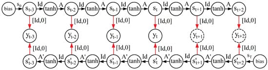
Figure 7.
Causal-retro-causal historically consistent neural network (CRCNN).
Architectural teacher forcing (ATF) for CRCNNs. CRCNNs are hard to train because they inherit all the characteristics from HCNNs. This implies that CRCNNs are also unfolded across the entire dataset, so the system has only one opportunity to learn from the whole history of the data. ATF makes the best possible use of the training data, accelerating and stabilizing the EBTT training process for the CRCNN. ATF replaces the outputs , up to time step , by the desired targets , and forces them into the causal network state and retro-causal network state .
Stabilizing information flows in dynamical systems. This is analogous to handling the uncertainty of the initial state for a basic RNN model with overshooting. The stability of the CRCNN model is further improved by applying noise in the causal as well as in the retro-causal branch of the network. The noise is injected into the same nodes that receive the biases (see Figure 7).
Uncertainty and risk. Traditional risk management applies diffusion models to interpret risk distributions. The risk can be explained as a random walk, in which, using the observed past error of the underlying model, the diffusion process is calibrated [161]. If the system identification calculation is performed using an HCNN or a CRCNN repeatedly, then solutions will be produced with a prediction error of zero in the past but that differ from each other in the future. If the arithmetic average of the individual ensemble members of the set is taken as the expected value, we will obtain a simplified prediction. Consider the bandwidth of the ensemble in addition to the expected value of Zimmermann, Tietz, and Grothmann [96]. The ensemble average can be taken as the best forecast, assuming that all future trajectories have the same probability and the genuine development of the dynamics is unknown, where the ensemble bandwidth describes the market risk. For any forecast date, all individual forecasts for the ensemble infer the probability distribution over many possible market prices at a single point in time, similar to an empirical density function.
4.6. Applying Echo State Networks to Time Series Forecasting
Training recurrent neural networks (RNNs) is a difficult task; however, they integrate a large dynamic memory and highly flexible computational capabilities, making them a very powerful tool. Error backpropagation (BP) is the standard method to train networks, especially feedforward neural networks (FFNNs), and it has also been extended to RNNs. This extension, however, has not been straightforward: RNNs are dynamical systems, and training them with BP sometimes leads to bifurcations, so chaos (non-convergence) occurs. Echo state networks (ESNs) are an alternative approach for training RNNs, as proposed by Jaeger [162]. In the classical ESN approach, an RNN structure is called a reservoir, so ESN methodology is often known in the literature as reservoir computing (RC), which is, at the moment, a prolific research area in RNNs [163]. In Lukoševičius [97], practical techniques and recommendations for successfully applying ESNs are presented, with emphasis on the time series forecasting problem. Lukoševičius [97] points out that ESNs are conceptually simple and easy to implement, but experience and insight are a must for training them successfully. In the remainder of this subsection, we summarize the main points addressed in this important contribution made by Lukoševičius [97].
The basic ESN model. ESNs are used to supervise temporal machine learning tasks where, for a given training input signal , a desired target output signal is known. The discrete time is and the number of data points in the training dataset is T. The task is to learn a model with output , where matches as best as possible, minimizing an error measure and, importantly, generalizing well to unseen data. The error measure E is typically a mean-squared error (MSE). The update equations are
and
where is a vector of reservoir neuron activations and is its update, all at time step n, is applied element-wise, stands for a vertical vector (or matrix) concatenation, and are the input and recurrent weight matrices, respectively, and is the leaking rate. It is important to mention here one fundamental difference between regular RNNs and ESNs: while ESN’s input and recurrent weight matrices and remain fixed once initialized, the weights in RNN’s state transition matrices are updated after each iteration during the learning process. A graphical representation of an ESN is depicted in Figure 8.
Figure 8.
An echo state network (ESN) in schematized form. is the training input signal, 1 is a constant input signal (intercept), contains input weights while contains recurrent weights (both and in the reservoir remain fixed after initialization), contains neuronal activations and is the reservoir’s output. are trainable output weights, and is the ESN’s output signal. weights minimize error after linear training.
The linear readout layer is defined as
where is the network output, and is the output weight matrix. The RC algorithm introduced with ESNs by Jaeger [162] consists of the following steps:
- Generate a random reservoir RNN ;
- Run the reservoir using the training input and collect the corresponding reservoir activation states ;
- Compute the linear readout weights from the reservoir, minimizing the MSE between and ;
- Use the trained network on new input data to compute by using the trained output weights .
Producing a reservoir. At the same time, the reservoir acts as a nonlinear expansion and as a memory of input . The reservoir can be described as a nonlinear, high-dimensional expansion of the input signal . For classification tasks, input data that are not linearly separable in the original space often become so in the expanded space of , where they are separated by .
Reservoir’s global parameters. Given the RNN models (33) and (34), the reservoir is defined by the tuple . The input and recurrent connection matrices and are generated randomly. The leaking rate of the reservoir nodes in (34) can be regarded as the speed of the reservoir update dynamics discretized in time.
Setup for parameter selection. Learning the results is fast in ESNs. This should be leveraged to evaluate how well a reservoir is generated by a particular set of parameters. To evaluate a reservoir, we train the output (35) and measure its error by applying cross-validation or training error. Randomly generated buckets, even with the same parameters, vary slightly in their performance. Keep the random seed fixed and averaged over multiple reservoir samples to eliminate random fluctuations in performance.
ESN ensemble. Training many small ESNs in parallel and averaging their outputs, in some cases, has drastically improved the performance of the basic ESN approach [164,165].
Removing initial transient. Usually data from the beginning of a long training sequence are discarded (i.e., not used for learning ) since they are contaminated by initial transients. The initial transient is a result of an arbitrary setting of , which is typically . An unnatural initial state is introduced that is not normally visited once the network has been “prepared” for the task. The number of time steps to discard depends on the network memory, which in turn depends on the reservoir parameters, and are normally at the order of tens or hundreds. From this, we see that regular RNNs (discussed in Section 4.5) and ESNs have differing approaches when dealing with the uncertainty of the initial state in the dynamical system they are trying to identify: RNNs inject noise into the initial state in order to identify a stable dynamical system, while ESNs discard a few initial transient states, relying on their echo state property to achieve stability.
5. Discussion
Statistical techniques, like linear regression, ARIMA, ARCH, and NARX modeling, have been traditionally employed in time series forecasting [166]. Strong assumptions on data are necessary for the construction of such models (e.g., data are generated by linear, time invariant processes, possibly with added Gaussian noise). These assumptions do not hold in many practical situations, and by using these traditional statistical techniques on time series from which we actually know very little about their true data-generating process, we incur the risk of generating inaccurate forecasts. Comparatively, ANN models offer a more flexible modeling strategy, with fewer assumptions on data-generating mechanisms, and produce accurate forecasts.
Generally speaking, the aim of time series forecasting is to predict future values with accuracy and simplicity. However, a large fraction of the ANN architectures reviewed in this article are more complex than others. But this fact seems to contradict the principle of Occam’s razor, which maintains that the simplest solution is usually the best. In machine learning literature, Occam’s razor is used for two different principles [167]:
- First razor: Starting from the fact that simplicity is desirable in itself, the simpler model should be preferred between two models with the same generalization error.
- Second razor: Starting from the fact that you are likely to have a smaller generalization error in the simpler model, it should be preferred between two models with the same error in the training set.
Domingos [167] argued that, in the first razor, simplicity is only a proxy for comprehensibility. Nevertheless, his paper shows that, contrary to the second razor’s claim, greater simplicity does not necessarily lead to greater accuracy. If we accept the fact that the most accurate models will not always be simple or easily understandable, we should allow an explicit trade-off between the two [167].
Occam’s razor is largely controversial. However, a simple and easy-to-understand method is needed to calculate point forecasts from machine learning time series models based on proven techniques.
6. Conclusions
Artificial neural networks (ANNs) have been (and still are) promising modeling techniques with an ever-increasing number of real-world applications. A very wide variety of ANN methods and algorithms are available; in fact, several tens of thousands of articles containing the keywords “time series” and “neural networks” can be found online. In this survey, we covered only a small and (hopefully) not-so-biased sample containing the most representative and popular ANN architectures employed for time series prediction tasks (for a small summary of surveyed studies, see Table 2). All the prototypical ANN architectures reviewed here constitute powerful, appealing machine learning techniques founded on sound mathematical and statistical principles. This is the reason why these methods work so well in many fields of study, including time series modeling and forecasting.
An interesting discussion that attempts to further explain from a theoretical perspective the success and power of ANNs (using concepts from probability and physics) can be found in Lin and Tegmark [168].
Table 2.
A small sample of ANN applications to time series forecasting tasks.
Table 2.
A small sample of ANN applications to time series forecasting tasks.
| Study | Main Model Employed | Time Series Forecasting Application |
|---|---|---|
| Adhikari et al. [81] | FFNN–PSO, Elman RNN–PSO | Macroeconomic variables |
| Alba-Cuéllar et al. [6] | FFNN–PSO ensemble-bootstrap | Monthly transportation data |
| Barrow and Crone [40] | FFNN ensembles | Transportation data |
| Blonbou [85] | Bayesian NN | Wind-generated power |
| Busseti et al. [169] | Deep RNN | Load forecasting |
| Chandra and Zhang [53] | Elman RNN | Chaotic time series |
| Chatzis and Demiris [170] | Bayesian ESN | Chaotic time series |
| Crone et al. [94] | FFNN, SVR | Monthly retail sales |
| Dablemont et al. [66] | Double SOM–RBFN | German DAX30 index |
| Giovanis [83] | FFNN–GA | Macroeconomic and financial data |
| Guo and Deng [89] | Hybrid FFNN–BP–ARIMA | Traffic flow |
| Jaeger and Haas [164] | ESN | Wireless communication signals |
| Jha et al. [80] | FFNN–PSO | Financial data |
| Kocadağlı and Aşıkgil [87] | Bayesian FFNN–GA | Weekly sales of a finance magazine |
| Lahmiri [41] | RBFN ensemble | NASDAQ returns |
| Leung et al. [114] | FFNN-improved GA | Natural phenomena (sunspots) |
| Maciel and Ballini [19] | FFNN | Stock market index forecasting |
| Mai et al. [48] | RBFN | Electric load |
| de M. Neto et al. [92] | FFNN–PSO | Financial data |
| Niu and Wang [47] | Improved RBFN | Financial data |
| Nourani et al. [68] | SOM–Wavelet Transform–FFNN | Satellite rainfall runoff data |
| Otok et al. [90] | Ensemble ARIMA–FFNN | Monthly rainfall in Indonesia |
| Sermpinis et al. [45] | RBFN–PSO | Global financial data |
| Shi and Han [171] | SVR–ESN hybrid | China Yellow River runoff |
| Simon et al. [64] | Double SOM | Polish electrical load time series |
| Skabar [84] | Bayesian FFNN | Australian Financial Index |
| Song [57] | Jordan RNN | Natural phenomena and sunspots |
| Valero et al. [63] | SOM, FFNN | Load demand in Spain electrical system |
| van Hinsbergen et al. [86] | Bayesian ANN | Urban travel time |
| Yadav and Srinivasan [65] | SOM–AR | Electricity demand in Britain and Wales |
| Yeh [93] | FFNN–ISSO | Natural phenomena and simulated data |
| Yin et al. [46] | RBFN | Tidal level at Canada’s west coast |
| Zhang [88] | Hybrid ARIMA–FFNN | Natural phenomena and financial data |
| Zhao et al. [54] | Elman RNN–Kalman filter | By-product gas flow in the steel industry |
| Zimmermann et al. [96] | ECNN | Demand of products and raw materials |
Feedforward-type ANN architectures (FFNNs, RBFNs, SOMs, SVRs, etc.) are by far the most popular among all ANN architectures employed for time series prediction tasks because of their relative simplicity, universal functional approximation properties, and stability. ANN training with alternative machine learning evolutionary algorithms (PSO, GA, ABC, etc.) and combined with ensemble modeling offers an attractive framework for producing accurate time series forecasts with associated uncertainty measures. Recurrent neural networks (RNNs) are hard to implement, but they are worth taking a look at, especially when we want to model long past time series behavior or when a time series behaves more like a chaotic dynamical system and less like a nonlinear autoregressive signal. RNN’s standard training algorithm (namely, error backpropagation through time) requires intensive computing resources and has to be handled carefully in order to achieve convergence and stability. On the other hand, the echo state network (ESN) approach to time series RNN modeling offers a faster way to identify stable dynamical systems since fast and economical linear regression aimed at selecting appropriate nonlinear neural activations is at the core of ESN training.
Especially in the early days (late 1980s and early 1990s), properly fitting a suitable ANN architecture to a given time series dataset in order to produce accurate forecasts was more of an art than a science. The building process of a time series ANN model relied heavily on trial and error and was very sensitive to the practitioner’s previous knowledge and experience with the data at hand. These limitations, together with seemingly conflicting empirical evidence regarding the forecasting power of ANNs, gave rise to doubts and skepticism about ANN’s overall ability to predict future time series values. In our opinion, the works surveyed in Section 4 define well-structured time series ANN modeling strategies that successfully address the aforementioned issues; however, work still needs to be done. Time series ANN modeling is not as well-established as traditional time series analysis due to the following:
- ANN modeling is still a fast-evolving field of study;
- Further work still needs to be done in order to employ ANNs as useful tools for understanding and interpreting relationships among time series variables involved in the forecasting task at hand (opening the black box);
- Although ensemble modeling and methods similar to the double SOM technique discussed in Section 4.4 provide solutions for quantifying the uncertainty of time series forecasts generated by ANN models, we think that work still needs to be done in order to construct statistically valid prediction intervals associated with time series point forecasts from ANN models.
On the other hand, traditional statistical linear regression models are simple to understand, easy to implement and interpret, and are always at the forefront of the time series modeling literature. Unfortunately, linear modeling offers only an incomplete framework since nonlinear features in temporal data play an important role in many time series forecasting tasks. Parametric nonlinear modeling is a difficult and cumbersome activity since many arbitrary initial assumptions have to be made about the true form of the unknown underlying data-generating process. Linear models are often used indiscriminately by many practitioners, even if the predictions turn out to be unsatisfactory, which is often the case given time series nonlinear characteristics for many real-world problems. People’s predisposition and willingness to ignore the limitations of traditional linear models is also an obstacle to the adoption of ANN techniques applied to time series forecasting tasks. Linear models, when used appropriately, are very effective tools. In fact, combining nonlinear methods based on ANNs with traditional linear models is a powerful and effective strategy. ESNs represent a prime example: linearly trained weights allow the ESN to select nonlinear neural activations from its reservoir. SOM models potentially offer a solution to the black-box problem associated with neural network models since their local approximation properties can be combined with linear time series modeling techniques, allowing users to study and interpret existing relationships among the response variable and some of its time-lagged values. An approach of our own to the problem of building statistically valid prediction intervals for time series point predictions generated by ANN models is outlined next: The basic idea is that, if a time series model has good generalization properties, then its forecasts will be close to actual future observations, and therefore the linear correlation coefficient between forecasts and true future observations (once they become available) will be close to one. Under these circumstances, it makes sense to build a simple linear regression model (called an auxiliary linear model) using validation data (i.e., the most recent observations in the training set) as the response variable and corresponding predictions from a fully trained ANN model (called the main ANN model) as the independent variable . Under favorable circumstances, the auxiliary linear model, after being built, would have a statistically insignificant intercept coefficient close to zero and a statistically significant slope coefficient close to one. The residuals from the auxiliary linear model would contain valuable information about the distribution of prediction errors associated with point forecasts generated by the main ANN model. Finally, we would employ our auxiliary linear model to compute standard errors associated with point forecasts generated by the main ANN model. These standard errors would be the basis for building prediction bands with a user-defined confidence level. In an upcoming paper, we will discuss our idea in more detail, putting to the test the associated hypotheses outlined here.
The recent big data phenomenon is now motivating researchers to take a closer look at machine learning techniques, specifically ANNs, which are well suited to huge time series datasets. Terabytes of satellite imaging data pour in constantly and incessantly. Such huge volumes of data would be impossible to analyze by traditional means. Machine learning techniques, including ANNs, become an essential tool in these situations since ANNs are good at identifying recurring patterns occurring in large volumes of data. The joint use of ANN and linear models applied to very large datasets with temporal structure could be a good opportunity for unifying traditional statistics and machine learning. Efforts should be made to standardize notation and techniques from both disciplines, so machine learning can be regarded by scientists and practitioners as an integral and important part of statistics.
Author Contributions
Conceptualization, A.E.M.-Z., J.E.M.-D., D.A.-C., and J.A.G.-D.-d.-L.; methodology, A.E.M.-Z., J.E.M.-D., D.A.-C., and J.A.G.-D.-d.-L.; software, A.E.M.-Z., J.E.M.-D., D.A.-C., and J.A.G.-D.-d.-L.; validation, A.E.M.-Z., J.E.M.-D., D.A.-C., and J.A.G.-D.-d.-L.; formal analysis, A.E.M.-Z., J.E.M.-D., D.A.-C., and J.A.G.-D.-d.-L.; investigation, A.E.M.-Z., J.E.M.-D., D.A.-C., and J.A.G.-D.-d.-L.; resources, A.E.M.-Z., J.E.M.-D., D.A.-C., and J.A.G.-D.-d.-L.; data curation, A.E.M.-Z., J.E.M.-D., D.A.-C., and J.A.G.-D.-d.-L.; writing—original draft preparation, A.E.M.-Z., J.E.M.-D., D.A.-C., and J.A.G.-D.-d.-L.; writing—review and editing, A.E.M.-Z., J.E.M.-D., D.A.-C., and J.A.G.-D.-d.-L.; visualization, A.E.M.-Z., J.E.M.-D., D.A.-C., and J.A.G.-D.-d.-L.; supervision, A.E.M.-Z., J.E.M.-D., D.A.-C., and J.A.G.-D.-d.-L.; project administration, A.E.M.-Z., J.E.M.-D., D.A.-C., and J.A.G.-D.-d.-L.; funding acquisition, J.E.M.-D. All authors have read and agreed to the published version of the manuscript.
Funding
This work was supported by the Universidad Autónoma de Aguascalientes through grant PII23-1. The corresponding author (J.E.M.-D.) was funded by the National Council of Science and Technology of Mexico (CONACYT) through grant A1-S-45928.
Institutional Review Board Statement
Not applicable.
Informed Consent Statement
Not applicable.
Data Availability Statement
Data sharing not applicable.
Acknowledgments
The authors wish to thank the anonymous reviewers for their comments and criticisms. All of their comments were taken into account in the revised version of the paper, resulting in a substantial improvement with respect to the original submission.
Conflicts of Interest
The authors declare no conflicts of interest.
Abbreviations
The following abbreviations are used in this manuscript:
| ABC | Artificial bee colony |
| ANN | Artificial Neural Network |
| ARCH | Autoregressive conditional heteroskedasticity |
| ARIMA | Autoregressive integrated moving average |
| BP | Backpropagation |
| BPTT | Backpropagation through time |
| CV | Cross-validation |
| FFNN | Feedforward neural networks |
| GA | Genetic algorithm |
| MLP | Multilayer perceptron |
| NARX | Nonlinear autoregressive with exogenous inputs |
| PEM | Prediction error measure |
| PCA | Principal component analysis |
| PSO | Particle swarm optimization |
| RBFN | Radial basis function network |
| RNN | Recurrent neural network |
| SOM | Self-organizing map |
| SVM | Support vector machines |
References
- Alba-Cuéllar, D.; Muñoz-Zavala, A.E. A Comparison between SARIMA Models and Feed Forward Neural Network Ensemble Models for Time Series Data. Res. Comput. Sci. 2015, 92, 9–22. [Google Scholar] [CrossRef]
- Panigrahi, R.; Patne, N.R.; Pemmada, S.; Manchalwar, A.D. Prediction of Electric Energy Consumption for Demand Response using Deep Learning. In Proceedings of the 2022 International Conference on Intelligent Controller and Computing for Smart Power (ICICCSP), Hyderabad, India, 21–23 July 2022; IEEE: New York, NY, USA, 2022; pp. 1–6. [Google Scholar]
- Wang, Y.; Chen, J.; Chen, X.; Zeng, X.; Kong, Y.; Sun, S.; Guo, Y.; Liu, Y. Short-Term Load Forecasting for Industrial Customers Based on TCN-LightGBM. IEEE Trans. Power Syst. 2021, 36, 1984–1997. [Google Scholar] [CrossRef]
- Tudose, A.M.; Picioroaga, I.I.; Sidea, D.O.; Bulac, C.; Boicea, V.A. Short-Term Load Forecasting Using Convolutional Neural Networks in COVID-19 Context: The Romanian Case Study. Energies 2021, 14, 4046. [Google Scholar] [CrossRef]
- Panigrahi, R.; Patne, N.; Surya Vardhan, B.; Khedkar, M. Short-term load analysis and forecasting using stochastic approach considering pandemic effects. Electr. Eng. 2023, in press. [Google Scholar] [CrossRef]
- Alba-Cuéllar, D.; Muñoz-Zavala, A.E.; Hernández-Aguirre, A.; Ponce-De-Leon-Senti, E.E.; Díaz-Díaz, E. Time Series Forecasting with PSO-Optimized Neural Networks. In Proceedings of the 2014 13th Mexican International Conference on Artificial Intelligence (MICAI), Tuxtla Gutierrez, Mexico, 16–22 November 2014; IEEE: New York, NY, USA, 2014; pp. 102–111. [Google Scholar]
- Box, G.E.; Jenkins, G.M. Time Series Analysis: Forecasting and Control; Holden Day: New York, NY, USA, 1970. [Google Scholar]
- Tong, H. Nonlinear time series analysis since 1990: Some personal reflections. Acta Math. Appl. Sin. 2002, 18, 177–184. [Google Scholar] [CrossRef]
- Tong, H. Non-Linear Time Series: A Dynamical System Approach; Oxford University Press: Oxford, UK, 1990. [Google Scholar]
- Engle, R.F. Autoregressive conditional heteroscedasticity with estimates of the variance of United Kingdom inflation. Econom. J. Econom. Soc. 1982, 50, 987–1007. [Google Scholar] [CrossRef]
- Granger, C.W.J.; Andersen, A.P. An Introduction to Bilinear Time Series Models; Vandenhoeck and Ruprecht: Göttingen, Germany, 1978. [Google Scholar]
- Murphy, K.P. Machine Learning: A Probabilistic Perspective; MIT Press: Cambridge, MA, USA, 2012. [Google Scholar]
- Drucker, H.; Burges, C.J.; Kaufman, L.; Smola, A.; Vapnik, V. Support vector regression machines. Adv. Neural Inf. Process. Syst. 1997, 9, 155–161. [Google Scholar]
- Härdle, W. Nonparametric and Semiparametric Models; Springer: Berlin/Heidelberg, Germany, 2004. [Google Scholar]
- McCulloch, W.S.; Pitts, W. A logical calculus of the ideas immanent in nervous activity. Bull. Math. Biophys. 1943, 5, 115–133. [Google Scholar] [CrossRef]
- Rosenblatt, F. The Perceptron—A Perceiving and Recognizing Automaton; Technical Report 85-460-1; Cornell Aeronautical Laboratory: Buffalo, NY, USA, 1957. [Google Scholar]
- Lapedes, A.; Farber, R. Nonlinear Signal Processing Using Neural Networks: Prediction and System Modeling; Technical Report LA-UR-87-2662; Los Alamos National Laboratory: Los Alamos, NM, USA, 1987. [Google Scholar]
- As’ad, F.; Farhat, C. A mechanics-informed deep learning framework for data-driven nonlinear viscoelasticity. Comput. Methods Appl. Mech. Eng. 2023, 417, 116463. [Google Scholar] [CrossRef]
- Maciel, L.S.; Ballini, R. Neural networks applied to stock market forecasting: An empirical analysis. Learn. Nonlinear Model. 2010, 8, 3–22. [Google Scholar] [CrossRef]
- Cybenko, G. Approximation by superpositions of a sigmoidal function. Math. Control Signals Syst. 1989, 2, 303–314. [Google Scholar] [CrossRef]
- Shumway, R.H.; Stoffer, D.S. Time Series Analysis and Its Applications (with R Examples), 3rd ed.; Springer Science+Business Media, LLC: Cham, Switzerland, 2011. [Google Scholar]
- Jones, E.R. An Introduction to Neural Networks: A White Paper; Visual Numerics Inc.: Houston, TX, USA, 2004. [Google Scholar]
- Touretzky, D.; Laskowski, K. Neural Networks for Time Series Prediction; Lecture Notes for Class 15-486/782: Artificial Neural Networks; Carnegie Mellon University: Pittsburgh, PA, USA, 2006. [Google Scholar]
- Whittle, P. Hypothesis Testing in Time Series Analysis; Hafner Publishing Company: New York, NY, USA, 1951. [Google Scholar]
- Box, G.E. Science and statistics. J. Am. Stat. Assoc. 1976, 71, 791–799. [Google Scholar] [CrossRef]
- Nisbet, B. Tutorial E—Feature Selection in KNIME. In Handbook of Statistical Analysis and Data Mining Applications, 2nd ed.; Nisbet, R., Miner, G., Yale, K., Eds.; Academic Press: Boston, MA, USA, 2018; pp. 377–391. [Google Scholar]
- Bullinaria, J.A. Neural Computation. 2014. Available online: https://www.cs.bham.ac.uk/~jxb/inc.html (accessed on 1 December 2023).
- Beale, R.; Jackson, T. Neural Computing—An Introduction; Institute of Physics Publishing: Bristol, UK, 1990. [Google Scholar]
- Bishop, C.M. Neural Networks for Pattern Recognition; Oxford University Press: Oxford, UK, 1995. [Google Scholar]
- Callan, R. Essence of Neural Networks; Prentice Hall PTR: Hoboken, NJ, USA, 1998. [Google Scholar]
- Fausett, L. Fundamentals of Neural Networks: Architectures, Algorithms, and Applications; Prentice Hall: Hoboken, NJ, USA, 1994. [Google Scholar]
- Gurney, K. An Introduction to Neural Networks; Routledge: London, UK, 1997. [Google Scholar]
- Ham, F.M.; Kostanic, I. Principles of Neurocomputing for Science and Engineering; McGraw-Hill Higher Education: New York, NY, USA, 2000. [Google Scholar]
- Haykin, S.S. Neural Networks and Learning Machines; Pearson Education Upper Saddle River: Hoboken, NJ, USA, 2009; Volume 3. [Google Scholar]
- Hertz, J. Introduction to the Theory of Neural Computation; Basic Books: New York, NY, USA, 1991; Volume 1. [Google Scholar]
- Mazaheri, P.; Rahnamayan, S.; Bidgoli, A.A. Designing Artificial Neural Network Using Particle Swarm Optimization: A Survey; IntechOpen: Rijeka, Croatia, 2022. [Google Scholar]
- Arlot, S.; Celisse, A. A survey of cross-validation procedures for model selection. Stat. Surv. 2010, 4, 40–79. [Google Scholar] [CrossRef]
- Hjorth, J.U. Computer Intensive Statistical Methods: Validation, Model Selection, and Bootstrap; Chapman and Hall: Boca Raton, FL, USA, 1994; pp. 65–73. [Google Scholar]
- Makridakis, S.; Winkler, R.L. Averages of forecasts: Some empirical results. Manag. Sci. 1983, 29, 987–996. [Google Scholar] [CrossRef]
- Barrow, D.K.; Crone, S.F. Crogging (cross-validation aggregation) for forecasting—A novel algorithm of neural network ensembles on time series subsamples. In Proceedings of the 2013 International Joint Conference on Neural Networks (IJCNN), Dallas, TX, USA, 4–9 August 2013; IEEE: New York, NY, USA, 2013; pp. 1–8. [Google Scholar]
- Lahmiri, S. Intelligent Ensemble Systems for Modeling NASDAQ Microstructure: A Comparative Study. In Artificial Neural Networks in Pattern Recognition; Springer: Cham, Switzerland, 2014; pp. 240–251. [Google Scholar]
- Broomhead, D.S.; Lowe, D. Radial Basis Functions, Multi-Variable Functional Interpolation and Adaptive Networks; Technical Report, DTIC Document; Controller HMSO: London, UK, 1988. [Google Scholar]
- Hartman, E.J.; Keeler, J.D.; Kowalski, J.M. Layered neural networks with Gaussian hidden units as universal approximations. Neural Comput. 1990, 2, 210–215. [Google Scholar] [CrossRef]
- Chang, W.Y. Wind energy conversion system power forecasting using radial basis function neural network. Appl. Mech. Mater. 2013, 284, 1067–1071. [Google Scholar] [CrossRef]
- Sermpinis, G.; Theofilatos, K.; Karathanasopoulos, A.; Georgopoulos, E.F.; Dunis, C. Forecasting foreign exchange rates with adaptive neural networks using radial-basis functions and Particle Swarm Optimization. Eur. J. Oper. Res. 2013, 225, 528–540. [Google Scholar] [CrossRef]
- Yin, J.c.; Zou, Z.j.; Xu, F. Sequential learning radial basis function network for real-time tidal level predictions. Ocean Eng. 2013, 57, 49–55. [Google Scholar] [CrossRef]
- Niu, H.; Wang, J. Financial time series prediction by a random data-time effective RBF neural network. Soft Comput. 2014, 18, 497–508. [Google Scholar] [CrossRef]
- Mai, W.; Chung, C.; Wu, T.; Huang, H. Electric load forecasting for large office building based on radial basis function neural network. In Proceedings of the 2014 IEEE PES General Meeting—Conference & Exposition, National Harbor, MD, USA, 27–31 July 2014; IEEE: New York, NY, USA, 2014; pp. 1–5. [Google Scholar]
- Zhu, J.Z.; Cao, J.X.; Zhu, Y. Traffic volume forecasting based on radial basis function neural network with the consideration of traffic flows at the adjacent intersections. Transp. Res. Part C Emerg. Technol. 2014, 47 Pt A, 139–154. [Google Scholar] [CrossRef]
- Elman, J.L. Finding structure in time. Cogn. Sci. 1990, 14, 179–211. [Google Scholar] [CrossRef]
- Sprott, J.C. Chaos and Time-Series Analysis; Oxford University Press: Oxford, UK, 2003; Volume 69. [Google Scholar]
- Ardalani-Farsa, M.; Zolfaghari, S. Chaotic time series prediction with residual analysis method using hybrid Elman–NARX neural networks. Neurocomputing 2010, 73, 2540–2553. [Google Scholar] [CrossRef]
- Chandra, R.; Zhang, M. Cooperative coevolution of Elman recurrent neural networks for chaotic time series prediction. Neurocomputing 2012, 86, 116–123. [Google Scholar] [CrossRef]
- Zhao, J.; Zhu, X.; Wang, W.; Liu, Y. Extended Kalman filter-based Elman networks for industrial time series prediction with GPU acceleration. Neurocomputing 2013, 118, 215–224. [Google Scholar] [CrossRef]
- Jordan, M.I. Attractor Dynamics and parallelism in a connectionist sequential machine. In Proceedings of the Eight Annual Conference of the Cognitive Science Society, Amherst, MA, USA, 15–17 August 1986; Lawrence Erlbaum Associates: Hillsdale, NJ, USA, 1986. [Google Scholar]
- Tabuse, M.; Kinouchi, M.; Hagiwara, M. Recurrent neural network using mixture of experts for time series processing. In Proceedings of the 1997 IEEE International Conference on Systems, Man, and Cybernetics—Computational Cybernetics and Simulation, Orlando, FL, USA,, 12–15 October 1997; IEEE: New York, NY, USA, 1997; Volume 1, pp. 536–541. [Google Scholar]
- Song, Q. Robust initialization of a Jordan network with recurrent constrained learning. Neural Netw. IEEE Trans. 2011, 22, 2460–2473. [Google Scholar] [CrossRef]
- Song, Q. Robust Jordan network for nonlinear time series prediction. In Proceedings of the 2011 International Joint Conference on Neural Networks (IJCNN), San Jose, CA, USA, 31 July–5 August 2011; IEEE: New York, NY, USA, 2011; pp. 2542–2549. [Google Scholar]
- Boussaada, Z.; Curea, O.; Remaci, A.; Camblong, H.; Mrabet Bellaaj, N. A Nonlinear Autoregressive Exogenous (NARX) Neural Network Model for the Prediction of the Daily Direct Solar Radiation. Energies 2018, 11, 620. [Google Scholar] [CrossRef]
- Kohonen, T. Self-Organizing Maps; Springer Series in Information Sciences; Springer: Berlin/Heidelberg, Germany, 1995; Volume 30. [Google Scholar]
- Barreto, G.A. Time series prediction with the self-organizing map: A review. In Perspectives of Neural-Symbolic Integration; Springer: Berlin/Heidelberg, Germany, 2007; pp. 135–158. [Google Scholar]
- Burguillo, J.C. Using self-organizing maps with complex network topologies and coalitions for time series prediction. Soft Comput. 2014, 18, 695–705. [Google Scholar] [CrossRef]
- Valero, S.; Aparicio, J.; Senabre, C.; Ortiz, M.; Sancho, J.; Gabaldon, A. Comparative analysis of Self Organizing Maps vs. multilayer perceptron neural networks for short-term load forecasting. In Proceedings of the Modern Electric Power Systems (MEPS), 2010 Proceedings of the International Symposium, Wroclaw, Poland, 20–22 September 2010; IEEE: New York, NY, USA, 2010; pp. 1–5. [Google Scholar]
- Simon, G.; Lendasse, A.; Cottrell, M.; Fort, J.C.; Verleysen, M. Double SOM for long-term time series prediction. In Proceedings of the Conference WSOM 2003, Kitakyushu, Japan, 11–14 September 2003; pp. 35–40. [Google Scholar]
- Yadav, V.; Srinivasan, D. Autocorrelation based weighing strategy for short-term load forecasting with the self-organizing map. In Proceedings of the 2010 the 2nd International Conference on Computer and Automation Engineering (ICCAE), Singapore, 26–28 February 2010; IEEE: New York, NY, USA, 2010; Volume 1, pp. 186–192. [Google Scholar]
- Dablemont, S.; Simon, G.; Lendasse, A.; Ruttiens, A.; Blayo, F.; Verleysen, M. Time series forecasting with SOM and local non-linear models—Application to the DAX30 index prediction. In Proceedings of the Workshop on Self-Organizing Maps, Kitakyushu, Japan, 11–14 September 2003. [Google Scholar]
- Cherif, A.; Cardot, H.; Boné, R. Recurrent Neural Networks as Local Models for Time Series Prediction. In Neural Information Processing; Springer: Berlin/Heidelberg, Germany, 2009; pp. 786–793. [Google Scholar]
- Nourani, V.; Baghanam, A.H.; Adamowski, J.; Gebremichael, M. Using self-organizing maps and wavelet transforms for space–time pre-processing of satellite precipitation and runoff data in neural network based rainfall–runoff modeling. J. Hydrol. 2013, 476, 228–243. [Google Scholar] [CrossRef]
- Bengio, Y.; Simard, P.; Frasconi, P. Learning long-term dependencies with gradient descent is difficult. IEEE Trans. Neural Netw. 1994, 5, 157–166. [Google Scholar] [CrossRef]
- Pascanu, R.; Mikolov, T.; Bengio, Y. On the difficulty of training Recurrent Neural Networks. In Proceedings of the 30th International Conference on Machine Learning, Atlanta, GA, USA, 16–21 June 2013; IEEE: New York, NY, USA, 2013. [Google Scholar]
- Hu, D.; Wu, R.; Chen, D.; Dou, H. An improved training algorithm of neural networks for time series forecasting. In MICAI 2007: Advances in Artificial Intelligence; Springer: Berlin/Heidelberg, Germany, 2007; pp. 550–558. [Google Scholar]
- Nunnari, G. An improved back propagation algorithm to predict episodes of poor air quality. Soft Comput. 2006, 10, 132–139. [Google Scholar] [CrossRef]
- Ioffe, S.; Szegedy, C. Batch normalization: Accelerating deep network training by reducing internal covariate shift. In Proceedings of the 32nd International Conference on International Conference on Machine Learning, ICML-2015, JMLR, Lille, France, 6–11 July 2015; pp. 448–456. [Google Scholar]
- Yang, G.; Pennington, J.; Rao, V.; Sohl-Dickstein, J.; Schoenholz, S.S. A Mean Field Theory of Batch Normalization; Cornell Uiversity: Ithaca, NY, USA, 2019. [Google Scholar]
- Werbos, P. Backpropagation through time: What it does and how to do it. Proc. IEEE 1990, 78, 1550–1560. [Google Scholar] [CrossRef]
- Hochreiter, S.; Schmidhuber, J. Long Short-Term Memory. Neural Comput. 1997, 9, 1735–1780. [Google Scholar] [CrossRef]
- Gers, F.A.; Schmidhuber, J.; Cummins, F. Learning to Forget: Continual Prediction with LSTM. Neural Comput. 2000, 12, 2451–2471. [Google Scholar] [CrossRef] [PubMed]
- Calin, O. Deep Learning Architectures: A Mathematical Approach; Springer: Cham, Switzerland, 2020. [Google Scholar]
- Roy, T.; kumar Shome, S. Optimization of RNN-LSTM Model Using NSGA-II Algorithm for IOT-based Fire Detection Framework. IETE J. Res. 2023, in press. [Google Scholar] [CrossRef]
- Jha, G.K.; Thulasiraman, P.; Thulasiram, R.K. PSO based neural network for time series forecasting. In Proceedings of the 2009 International Joint Conference on Neural Networks, IJCNN 2009, Atlanta, GA, USA, 14–19 June 2009; IEEE: New York, NY, USA, 2009; pp. 1422–1427. [Google Scholar]
- Adhikari, R.; Agrawal, R.; Kant, L. PSO based Neural Networks vs. traditional statistical models for seasonal time series forecasting. In Proceedings of the 2013 3rd IEEE International Advance Computing Conference (IACC), Ghaziabad, India, 22–23 February 2013; IEEE: New York, NY, USA, 2013; pp. 719–725. [Google Scholar]
- Awan, S.M.; Aslam, M.; Khan, Z.A.; Saeed, H. An efficient model based on artificial bee colony optimization algorithm with Neural Networks for electric load forecasting. Neural Comput. Appl. 2014, 25, 1967–1978. [Google Scholar] [CrossRef]
- Giovanis, E. Feed-Forward Neural Networks Regressions with Genetic Algorithms: Applications in Econometrics and Finance. SSRN 2010, in press. [Google Scholar] [CrossRef]
- Skabar, A.A. Direction-of-change financial time series forecasting using neural networks: A Bayesian approach. In Advances in Electrical Engineering and Computational Science; Springer: Dordrecht, The Netherlands, 2009; pp. 515–524. [Google Scholar]
- Blonbou, R. Very short-term wind power forecasting with neural networks and adaptive Bayesian learning. Renew. Energy 2011, 36, 1118–1124. [Google Scholar] [CrossRef]
- Van Hinsbergen, C.; Hegyi, A.; van Lint, J.; van Zuylen, H. Bayesian neural networks for the prediction of stochastic travel times in urban networks. IET Intell. Transp. Syst. 2011, 5, 259–265. [Google Scholar] [CrossRef]
- Kocadağlı, O.; Aşıkgil, B. Nonlinear time series forecasting with Bayesian neural networks. Expert Syst. Appl. 2014, 41, 6596–6610. [Google Scholar] [CrossRef]
- Zhang, G.P. Time series forecasting using a hybrid ARIMA and neural network model. Neurocomputing 2003, 50, 159–175. [Google Scholar] [CrossRef]
- Guo, X.; Deng, F. Short-term prediction of intelligent traffic flow based on BP neural network and ARIMA model. In Proceedings of the 2010 International Conference on E-Product E-Service and E-Entertainment (ICEEE), Henan, China, 7–9 November 2010; IEEE: New York, NY, USA, 2010; pp. 1–4. [Google Scholar]
- Otok, B.W.; Lusia, D.A.; Faulina, R.; Kuswanto, H. Ensemble method based on ARIMA-FFNN for climate forecasting. In Proceedings of the 2012 International Conference on Statistics in Science, Business, and Engineering (ICSSBE), Langkawi, Malaysia, 10–12 September 2012; IEEE: New York, NY, USA, 2012; pp. 1–4. [Google Scholar]
- Viviani, E.; Di Persio, L.; Ehrhardt, M. Energy Markets Forecasting. From Inferential Statistics to Machine Learning: The German Case. Energies 2021, 14, 364. [Google Scholar] [CrossRef]
- Neto, P.S.d.M.; Petry, G.G.; Aranildo, R.L.J.; Ferreira, T.A.E. Combining artificial neural network and particle swarm system for time series forecasting. In Proceedings of the 2009 International Joint Conference on Neural Networks, IJCNN 2009, Atlanta, GA, USA, 14–19 June 2009; IEEE: New York, NY, USA, 2009; pp. 2230–2237. [Google Scholar]
- Yeh, W.C. New Parameter-Free Simplified Swarm Optimization for Artificial Neural Network Training and its Application in the Prediction of Time Series. IEEE Trans. Neural Netw. Learn. Syst. 2013, 24, 661–665. [Google Scholar]
- Crone, S.F.; Guajardo, J.; Weber, R. A study on the ability of support vector regression and neural networks to forecast basic time series patterns. In Artificial Intelligence in Theory and Practice; Springer: Boston, MA, USA, 2006; pp. 149–158. [Google Scholar]
- Moody, J. Forecasting the economy with neural nets: A survey of challenges and solutions. In Neural Networks: Tricks of the Trade, 2nd ed.; Montavon, G., Orr, G.B., Müller, K.R., Eds.; Lecture Notes in Computer Science; Springer: Berlin/Heidelberg, Germany, 2012; Volume 7700, pp. 343–367. [Google Scholar]
- Zimmermann, H.G.; Tietz, C.; Grothmann, R. Forecasting with recurrent neural networks: 12 tricks. In Neural Networks: Tricks of the Trade; Springer: Berlin/Heidelberg, Germany, 2012; pp. 687–707. [Google Scholar]
- Lukoševičius, M. A practical guide to applying echo state networks. In Neural Networks: Tricks of the Trade; Springer: Berlin/Heidelberg, Germany, 2012; pp. 659–686. [Google Scholar]
- Holland, J.H. Adaptation in Natural and Artificial Systems; University of Michigan Press: Ann Arbor, MI, USA, 1975. [Google Scholar]
- Angeline, P.J. Evolutionary optimization versus particle swarm optimization: Philosophy and performance differences. In Evolutionary Programming VII; Springer: Berlin/Heidelberg, Germany, 1998; pp. 601–610. [Google Scholar]
- Freitas, D.; Lopes, L.G.; Morgado-Dias, F. Particle Swarm Optimisation: A Historical Review Up to the Current Developments. Entropy 2020, 22, 362. [Google Scholar] [CrossRef]
- Kennedy, J.; Eberhart, R. Particle swarm optimization. In Proceedings of the IEEE International Conference on Neural Networks, Perth, WA, Australia, 27 November–1 December 1995; IEEE: New York, NY, USA, 1995; Volume 4, pp. 1942–1948. [Google Scholar]
- Eberhart, R.; Shi, Y. Evolving Artificial Neural Networks. In Proceedings of the International Conference on Neural Networks and Brain, PRC, Anchorage, AK, USA, 4–9 May 1998; Volume 1, pp. PL5–PL13. [Google Scholar]
- Eberhart, R.; Shi, Y. Particle swarm optimization: Developments, applications and resources. In Proceedings of the 2001 Congress on Evolutionary Computation, Seoul, Republic of Korea, 27–30 May 2001; IEEE: New York, NY, USA, 2001; Volume 1, pp. 81–86. [Google Scholar]
- Yu, J.; Wang, S.; Xi, L. Evolving artificial neural networks using an improved PSO and DPSO. Neurocomputing 2008, 71, 1054–1060. [Google Scholar] [CrossRef]
- Munoz-Zavala, A.E. A Comparison Study of PSO Neighborhoods. In EVOLVE—A Bridge between Probability, Set Oriented Numerics, and Evolutionary Computation II; Springer: Berlin/Heidelberg, Germany, 2013; pp. 251–265. [Google Scholar]
- Eberhart, R.; Dobbins, R.; Simpson, P. Computational Intelligence PC Tools; Academic Press Professional: Cambridge, MA, USA, 1996. [Google Scholar]
- Clerc, M.; Kennedy, J. The particle swarm: Explosion, stability, and convergence in a multidimensional complex space. IEEE Trans. Evol. Comput. 2002, 6, 58–73. [Google Scholar] [CrossRef]
- Slama, S.; Errachdi, A.; Benrejeb, M. Tuning Artificial Neural Network Controller Using Particle Swarm Optimization Technique for Nonlinear System; IntechOpen: Rijeka, Croatia, 2021. [Google Scholar]
- Ahmadzadeh, E.; Lee, J.; Moon, I. Optimized Neural Network Weights and Biases Using Particle Swarm Optimization Algorithm for Prediction Applications. J. Korea Multimed. Soc. 2017, 20, 1406–1420. [Google Scholar]
- Hagan, M.T.; Menhaj, M.B. Training feedforward networks with the Marquardt algorithm. Neural Netw. IEEE Trans. 1994, 5, 989–993. [Google Scholar] [CrossRef] [PubMed]
- Riedmiller, M.; Braun, H. A direct adaptive method for faster backpropagation learning: The RPROP algorithm. In Proceedings of the IEEE International Conference on Neural Networks, San Francisco, CA, USA, 28 March–1 April 1993; IEEE: New York, NY, USA, 1993; pp. 586–591. [Google Scholar]
- Møller, M.F. A scaled conjugate gradient algorithm for fast supervised learning. Neural Netw. 1993, 6, 525–533. [Google Scholar] [CrossRef]
- Battiti, R. One step secant conjugate gradient. Neural Comput. 1992, 4, 141–166. [Google Scholar] [CrossRef]
- Leung, F.H.F.; Lam, H.K.; Ling, S.H.; Tam, P.K.S. Tuning of the structure and parameters of a neural network using an improved genetic algorithm. IEEE Trans. Neural Netw. 2003, 14, 79–88. [Google Scholar] [CrossRef]
- Sitte, R.; Sitte, J. Neural networks approach to the random walk dilemma of financial time series. Appl. Intell. 2002, 16, 163–171. [Google Scholar] [CrossRef]
- de Araujo, R.; Madeiro, F.; de Sousa, R.P.; Pessoa, L.F.; Ferreira, T. An evolutionary morphological approach for financial time series forecasting. In Proceedings of the 2006 IEEE Congress on Evolutionary Computation, CEC 2006, Vancouver, BC, Canada, 16–21 July 2006; IEEE: New York, NY, USA, 2006; pp. 2467–2474. [Google Scholar]
- Yeh, W.C.; Chang, W.W.; Chung, Y.Y. A new hybrid approach for mining breast cancer pattern using discrete particle swarm optimization and statistical method. Expert Syst. Appl. 2009, 36, 8204–8211. [Google Scholar] [CrossRef]
- Goldberg, D.E. Genetic Algorithms in Search, Optimization, and Machine Learning; Addison-Wesley: Boston, MA, USA, 1989. [Google Scholar]
- Zhao, L.; Yang, Y. PSO-based single multiplicative neuron model for time series prediction. Expert Syst. Appl. 2009, 36, 2805–2812. [Google Scholar] [CrossRef]
- Mackey, M.C.; Glass, L. Oscillation and chaos in physiological control systems. Science 1977, 197, 287–289. [Google Scholar] [CrossRef] [PubMed]
- Hyndman, R. Time Series Data Library. 2014. Available online: https://robjhyndman.com/tsdl/ (accessed on 1 December 2023).
- Keirn, Z. EEG Pattern Analysis. 1988. Available online: https://github.com/meagmohit/EEG-Datasets (accessed on 1 December 2023).
- Gershenfeld, N.; Weigend, A. The Santa Fe Time Series Competition Data. 1994. Available online: http://techlab.bu.edu/resources/data_view/the_santa_fe_time_series_competition_data/index.html (accessed on 1 December 2023).
- Gudise, V.; Venayagamoorthy, G. Comparison of particle swarm optimization and backpropagation as training algorithms for neural networks. In Proceedings of the 2003 IEEE Swarm Intelligence Symposium. SIS’03 (Cat. No. 03EX706), Indianapolis, IN, USA, 26 April 2003; IEEE: New York, NY, USA, 2003; pp. 110–117. [Google Scholar]
- Liu, C.; Ding, W.; Li, Z.; Yang, C. Prediction of High-Speed Grinding Temperature of Titanium Matrix Composites Using BP Neural Network Based on PSO Algorithm. Int. J. Adv. Manuf. Technol. 2016, 89, 2277–2285. [Google Scholar] [CrossRef]
- Ince, T.; Kiranyaz, S.; Gabbouj, M. A Generic and Robust System for Automated Patient-Specific Classification of ECG Signals. IEEE Trans. Biomed. Eng. 2009, 56, 1415–1426. [Google Scholar] [CrossRef]
- Hamed, H.N.A.; Shamsuddin, S.M.; Salim, N. Particle Swarm Optimization For Neural Network Learning Enhancement. J. Teknol. 2008, 49, 13–26. [Google Scholar]
- Olayode, I.O.; Tartibu, L.K.; Okwu, M.O.; Ukaegbu, U.F. Development of a Hybrid Artificial Neural Network-Particle Swarm Optimization Model for the Modelling of Traffic Flow of Vehicles at Signalized Road Intersections. Appl. Sci. 2021, 11, 8387. [Google Scholar] [CrossRef]
- Van den Bergh, F.; Engelbrecht, A. Cooperative learning in neural networks using particle swarm optimizers. S. Afr. Comput. J. 2000, 2000, 84–90. [Google Scholar]
- van den Bergh, F.; Engelbrecht, A. Training product unit networks using cooperative particle swarm optimisers. In Proceedings of the International Joint Conference on Neural Networks, IJCNN’01, Washington, DC, USA, 15–19 July 2001; IEEE: New York, NY, USA, 2001; Volume 1, pp. 126–131. [Google Scholar]
- Munoz-Zavala, A.; Hernandez-Aguirre, A.; Villa Diharce, E. Constrained optimization via particle evolutionary swarm optimization algorithm (PESO). In Proceedings of the 7th Annual Conference on Genetic and Evolutionary Computation, GECCO’05, Washington, DC, USA, 25–99 June 2005; ACM: New York, NY, USA, 2005; pp. 209–216. [Google Scholar]
- Munoz-Zavala, A.; Hernandez-Aguirre, A.; Villa Diharce, E.; Botello Rionda, S. Constrained optimization with an improved particle swarm optimization algorithm. Int. J. Intell. Comput. Cybern. 2008, 1, 425–453. [Google Scholar] [CrossRef]
- Kennedy, J. Methods of agreement: Inference among the EleMentals. In Proceedings of the 1998 IEEE International Symposium on Intelligent Control (ISIC) Held Jointly with IEEE International Symposium on Computational Intelligence in Robotics and Automation (CIRA) Intell, Gaithersburg, MD, USA, 17 September 1998; IEEE: New York, NY, USA, 1998; pp. 883–887. [Google Scholar]
- Ozcan, E.; Mohan, C. Analysis of a Simple Particle Swarm Optimization System. Intell. Eng. Syst. Artif. Neural Netw. 1998, 8, 253–258. [Google Scholar]
- Van den Bergh, F.; Engelbrecht, A.P. A Convergence Proof for the Particle Swarm Optimiser. Fundam. Inform. 2010, 105, 341–374. [Google Scholar] [CrossRef]
- Kan, W.; Jihong, S. The Convergence Basis of Particle Swarm Optimization. In Proceedings of the 2012 International Conference on Industrial Control and Electronics Engineering, Xi’an, China, 23–25 August 2012; IEEE: New York, NY, USA, 2012; pp. 63–66. [Google Scholar]
- Qian, W.; Li, M. Convergence analysis of standard particle swarm optimization algorithm and its improvement. Soft Comput. 2018, 22, 4047–4070. [Google Scholar] [CrossRef]
- Xu, G.; Yu, G. On convergence analysis of particle swarm optimization algorithm. J. Comput. Appl. Math. 2018, 333, 65–73. [Google Scholar] [CrossRef]
- Huang, H.; Qiu, J.; Riedl, K. On the Global Convergence of Particle Swarm Optimization Methods. Appl. Math. Optim. 2023, 88, 30. [Google Scholar] [CrossRef]
- Zhang, G.P.; Qi, M. Neural network forecasting for seasonal and trend time series. Eur. J. Oper. Res. 2005, 160, 501–514. [Google Scholar] [CrossRef]
- Vapnik, V.N. The Nature of Statistical Learning Theory; Springer-Verlag New York, Inc.: New York, NY, USA, 1995. [Google Scholar]
- US Census Bureau. X-13ARIMA-SEATS Seasonal Adjustment Program. 2016. Available online: https://www.census.gov/srd/www/x13as/ (accessed on 22 October 2016).
- Kiani, K.M. On business cycle fluctuations in USA macroeconomic time series. Econ. Model. 2016, 53, 179–186. [Google Scholar] [CrossRef]
- Moody, J. Prediction risk and neural network architecture selection. In From Statistics to Neural Networks: Theory and Pattern Recognition Applications; Cherkassky, V., Friedman, J.H., Wechsler, H., Eds.; Springer: Berlin/Heidelberg, Germany, 1994; pp. 147–165. [Google Scholar]
- Pi, H.; Peterson, C. Finding the embedding dimension and variable dependencies in time series. Neural Comput. 1994, 6, 509–520. [Google Scholar] [CrossRef]
- Yang, H.; Moody, J. Input Variable Selection Based on Joint Mutual Information; Technical Report; Department of Computer Science, Oregon Graduate Institute: Eugene, OR, USA, 1998. [Google Scholar]
- Mozer, M.C.; Smolensky, P. Skeletonization: A technique for trimming the fat from a network via relevance assessment. In Advances in Neural Information Processing Systems; ACM: New York, NY, USA, 1989; pp. 107–115. [Google Scholar]
- Ash, T. Dynamic node creation in backpropagation networks. Connect. Sci. 1989, 1, 365–375. [Google Scholar] [CrossRef]
- LeCun, Y.; Denker, J.S.; Solla, S.A.; Howard, R.E.; Jackel, L.D. Optimal brain damage. Adv. Neural Inf. Process. Syst. 1989, 2, 598–605. [Google Scholar]
- Hassibi, B.; Stork, D.G. Second order derivatives for network pruning: Optimal brain surgeon. Adv. Neural Inf. Process. Syst. 1993, 5, 164. [Google Scholar]
- Levin, A. Fast pruning using principal components. Adv. Neural Inf. Process. Syst. 1994, 6, 35–42. [Google Scholar]
- Moody, J.E.; Rögnvaldsson, T. Smoothing Regularizers for Projective Basis Function Networks. Adv. Neural Inf. Process. Syst. 1996, 9, 585–591. [Google Scholar]
- Wu, L.; Moody, J. A smoothing regularizer for feedforward and recurrent neural networks. Neural Comput. 1996, 8, 461–489. [Google Scholar] [CrossRef]
- Liao, Y.; Moody, J. A neural network visualization and sensitivity analysis toolkit. In Proceedings of the International Conference on Neural Information Processing (ICONIP’96), Hong Kong, China, 24–27 September 1996; Amari, S.-I., Xu, L., Chan, L., King, I., Leung, K.-S., Eds.; Springer Verlag Singapore Pte. Ltd.: Singapore, 1996; pp. 1069–1074. [Google Scholar]
- Schäfer, A.M.; Zimmermann, H.G. Recurrent neural networks are universal approximators. In Artificial Neural Networks–ICANN 2006; Springer: Berlin/Heidelberg, Germany, 2006; pp. 632–640. [Google Scholar]
- Rumelhart, D.E.; Hinton, G.E.; Williams, R.J. Learning Internal Representations by Error Propagation; Technical Report, DTIC Document; Institute for Cognitive Science University of California: San Diego, CA, USA, 1985. [Google Scholar]
- Zimmermann, H.G.; Neuneier, R. Neural network architectures for the modeling of dynamical systems. In A Field Guide to Dynamical Recurrent Networks; Wiley-IEEE Press: Hoboken, NJ, USA, 2001; pp. 311–350. [Google Scholar]
- Werbos, P. Beyond Regression: New Tools for Prediction and Analysis in the Behavioral Sciences. Ph.D. Thesis, Harvard University, Cambridge, MA, USA, 1974. [Google Scholar]
- Zimmermann, H.G.; Neuneier, R.; Grothmann, R. Modeling dynamical systems by error correction neural networks. In Modelling and Forecasting Financial Data; Springer: Boston, MA, USA, 2002; pp. 237–263. [Google Scholar]
- Zimmermann, H.G.; Grothmann, R.; Schäfer, A.M.; Tietz, C.; Georg, H. Modeling Large Dynamical Systems with Dynamical Consistent Neural Networks. In New Directions in Statistical Signal Processing; MIT Press: Cambridge, MA, USA, 2007; p. 203. [Google Scholar]
- McNeil, A.J.; Frey, R.; Embrechts, P. Quantitative Risk Management: Concepts, Techniques, and Tools; Princeton University Press: Princeton, NJ, USA, 2010. [Google Scholar]
- Jaeger, H. The “Echo State” Approach to Analysing and Training Recurrent Neural Networks—With an Erratum Note; GMD Technical Report 148; German National Research Center for Information Technology: Bonn, Germany, 2001; p. 13. [Google Scholar]
- Jaeger, H. Echo state network. Scholarpedia 2007, 2, 2330. [Google Scholar] [CrossRef]
- Jaeger, H.; Haas, H. Harnessing nonlinearity: Predicting chaotic systems and saving energy in wireless communication. Science 2004, 304, 78–80. [Google Scholar] [CrossRef] [PubMed]
- Jaeger, H.; Lukoševičius, M.; Popovici, D.; Siewert, U. Optimization and applications of echo state networks with leaky-integrator neurons. Neural Netw. 2007, 20, 335–352. [Google Scholar] [CrossRef]
- Hyndman, R.; Athanasopoulos, G. Forecasting: Principles and Practice; OTexts: Melbourne, VIC, Australia, 2021; Volume 1. [Google Scholar]
- Domingos, P. Occam’s Two Razors: The Sharp and the Blunt. In Proceedings of the Fourth International Conference on Knowledge Discovery and Data Mining, New York, NY, USA, 27–31 August 1998; ACM: New York, NY, USA; AAAI Press: Washington, DC, USA, 1998; pp. 37–43. [Google Scholar]
- Lin, H.W.; Tegmark, M. Why does deep and cheap learning work so well? arXiv 2016, arXiv:1608.08225. [Google Scholar] [CrossRef]
- Busseti, E.; Osband, I.; Wong, S. Deep Learning for Time Series Modeling; Technical Report; Stanford University: Stanford, CA, USA, 2012. [Google Scholar]
- Chatzis, S.P.; Demiris, Y. Echo state Gaussian process. Neural Netw. IEEE Trans. 2011, 22, 1435–1445. [Google Scholar] [CrossRef]
- Shi, Z.; Han, M. Support vector echo-state machine for chaotic time-series prediction. Neural Netw. IEEE Trans. 2007, 18, 359–372. [Google Scholar] [CrossRef]
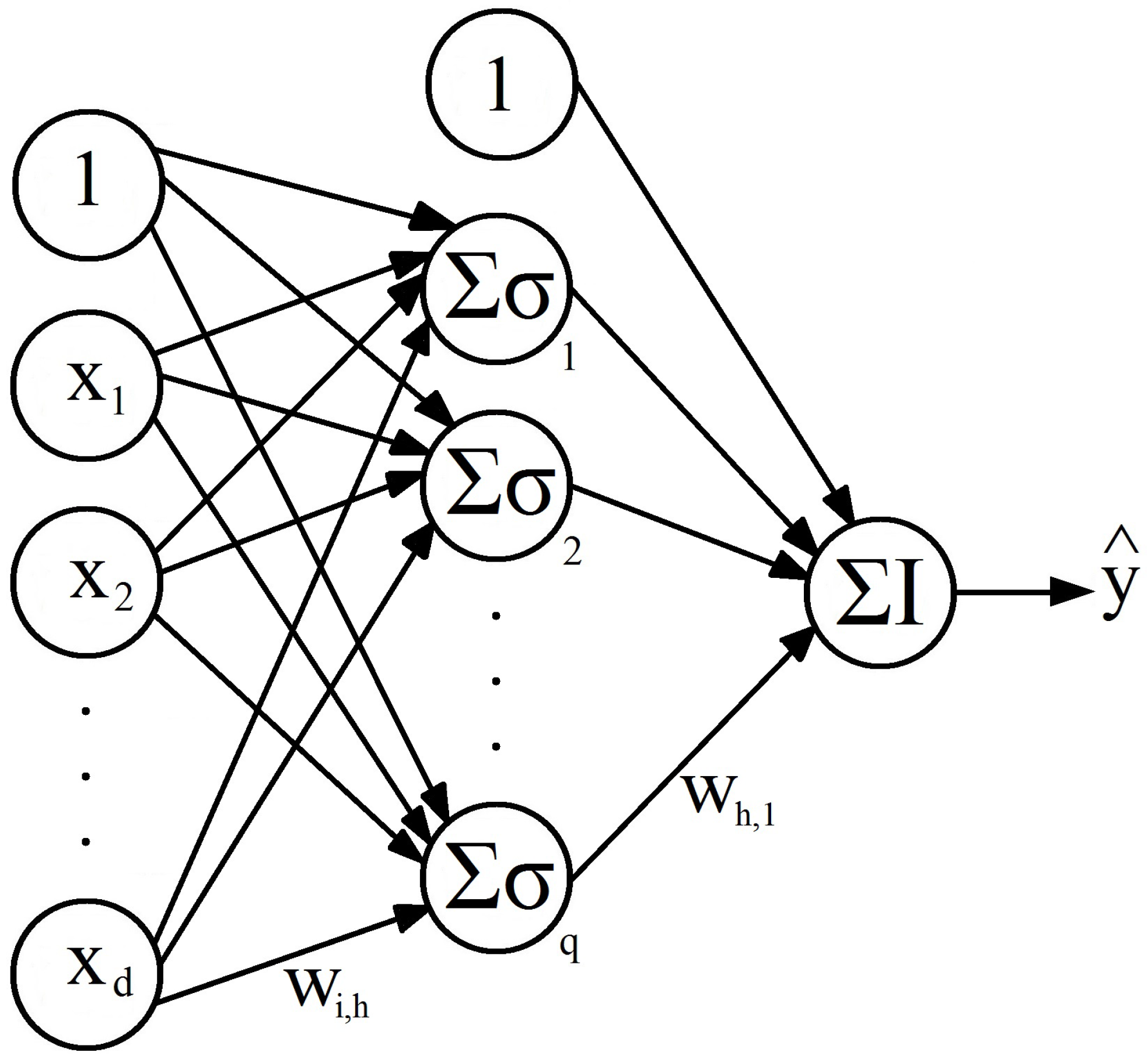

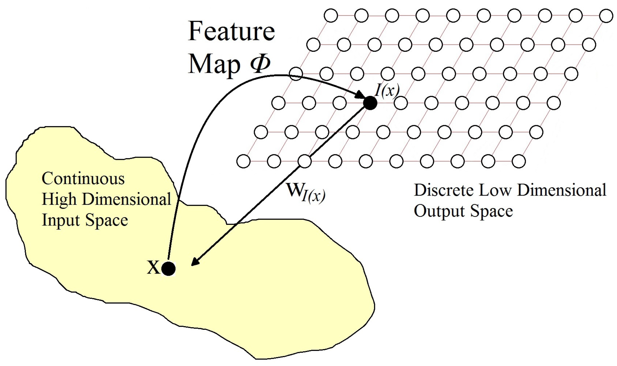
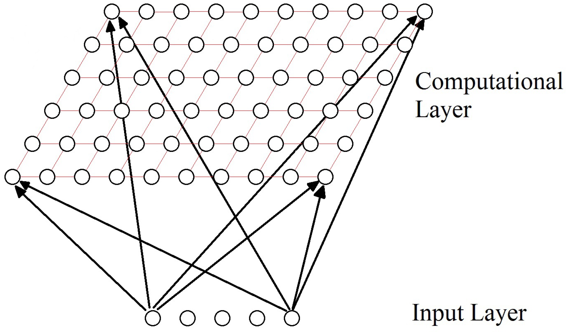
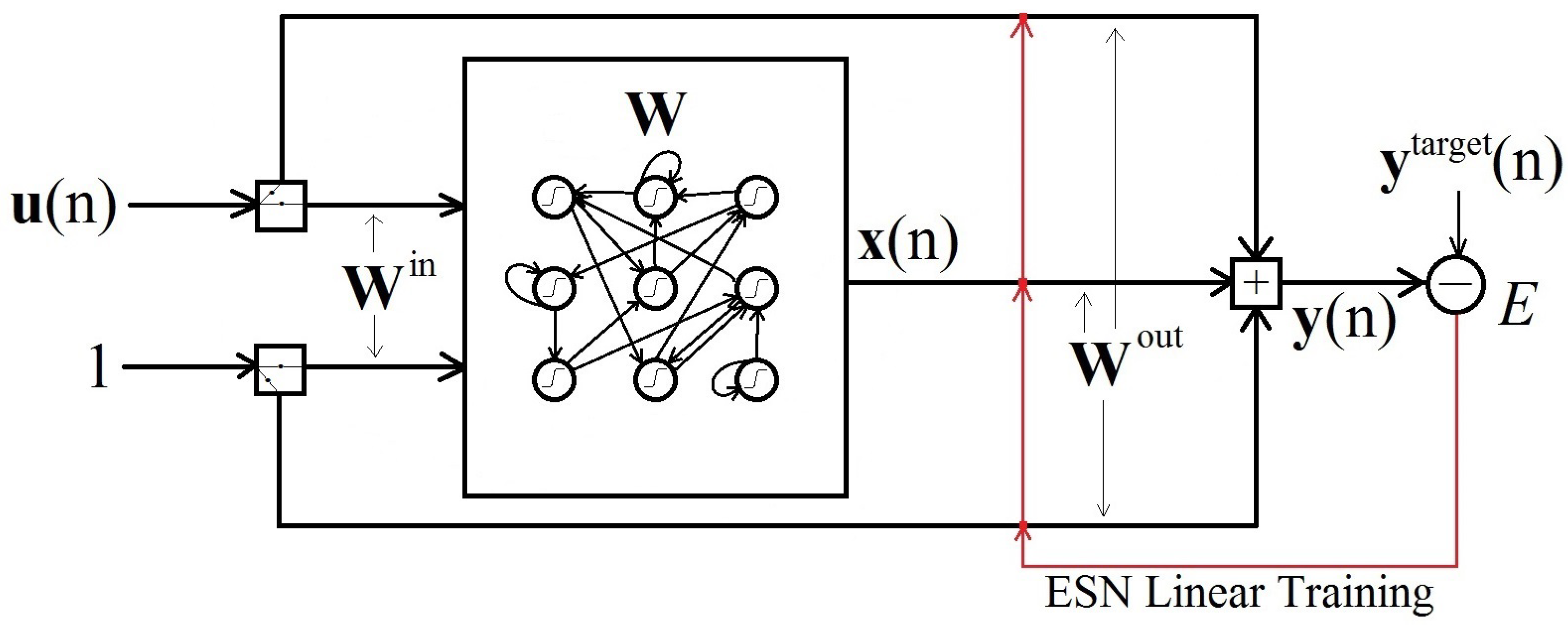
Disclaimer/Publisher’s Note: The statements, opinions and data contained in all publications are solely those of the individual author(s) and contributor(s) and not of MDPI and/or the editor(s). MDPI and/or the editor(s) disclaim responsibility for any injury to people or property resulting from any ideas, methods, instructions or products referred to in the content. |
© 2024 by the authors. Licensee MDPI, Basel, Switzerland. This article is an open access article distributed under the terms and conditions of the Creative Commons Attribution (CC BY) license (https://creativecommons.org/licenses/by/4.0/).