Article

GPU Adding-Doubling Algorithm for Analysis of Optical Spectral Images

1
Faculty of Mathematics and Physics, University of Ljubljana, SI-1000 Ljubljana, Slovenia
2
Jozef Stefan Institute, SI-1000 Ljubljana, Slovenia
3
Institute of Mathematics, Physics, and Mechanics, SI-1000 Ljubljana, Slovenia
4
Syreon Research Institute, 1145 Budapest, Hungary
*
Author to whom correspondence should be addressed.
Algorithms 2024, 17(2), 74; https://doi.org/10.3390/a17020074
Submission received: 26 December 2023 / Revised: 31 January 2024 / Accepted: 4 February 2024 / Published: 7 February 2024

Abstract

:
The Adding-Doubling (AD) algorithm is a general analytical solution of the radiative transfer equation (RTE). AD offers a favorable balance between accuracy and computational efficiency, surpassing other RTE solutions, such as Monte Carlo (MC) simulations, in terms of speed while outperforming approximate solutions like the Diffusion Approximation method in accuracy. While AD algorithms have traditionally been implemented on central processing units (CPUs), this study focuses on leveraging the capabilities of graphics processing units (GPUs) to achieve enhanced computational speed. In terms of processing speed, the GPU AD algorithm showed an improvement by a factor of about 5000 to 40,000 compared to the GPU MC method. The optimal number of threads for this algorithm was found to be approximately 3000. To illustrate the utility of the GPU AD algorithm, the Levenberg–Marquardt inverse solution was used to extract object parameters from optical spectral data of human skin under various hemodynamic conditions. With regards to computational efficiency, it took approximately 5 min to process a 220 × 100 × 61 image (x-axis × y-axis × spectral-axis). The development of the GPU AD algorithm presents an advancement in determining tissue properties compared to other RTE solutions. Moreover, the GPU AD method itself holds the potential to expedite machine learning techniques in the analysis of spectral images.

1. Introduction

Building on Stokes’ method to calculate the transmission of light through a pile of plates [1], van de Hulst [2] in 1962 proposed the Adding-Doubling (AD) algorithm, an efficient technique to solve the radiative transfer equation (RTE) within complex media, such as clouds, aerosols, and biological tissues. Numerous studies have adopted the AD algorithm to advance our understanding of atmospheric processes and remote sensing applications [3,4,5], luminescence in solar cells [6], biomedical optics [7,8], and photovoltaic and nuclear reactor research [9,10,11].
Briefly, the AD algorithm consists of two essential components: the Doubling method and the Adding method [12,13]. The Doubling method relies on prior knowledge of the reflection and transmission properties of a single thin homogeneous layer. By combining two identical slabs and summing their individual contributions, the reflection and transmission of a slab that is twice as thick can be determined. This doubling process is then iteratively applied, progressively increasing the slab’s thickness until the desired magnitude is achieved. The Adding method extends the Doubling method by allowing for the simulation of media that consist of diverse layers and involve instances of internal reflection at boundaries. By incorporating dissimilar slabs into the calculations, we can achieve a more comprehensive representation of complex media structures.
Understanding the interaction of photons with biological tissues holds immense importance in various fields, including medical imaging, diagnostics, and laser therapy. To model this intricate process, two widely used approaches are the Monte Carlo (MC) method [14] and the AD algorithm [13]. The MC method is a statistical technique that simulates photon transport by creating random photon paths within the tissue. It uses probabilistic calculations to model absorption, scattering, and reflection/refraction events based on the tissue’s optical properties. Starting from an initial position and direction, photons are randomly sampled and tracked as they interact with the tissue. At each interaction, the path length and probability of scattering or absorption are considered, allowing the simulation to replicate the complex behavior of photons in a stochastic manner. The MC method offers several advantages, including its flexibility to simulate complex geometries and heterogeneous tissue structures. It is particularly adept at capturing intricate molecular and cellular photon interactions, making it valuable for biological and medical research. However, due to its statistical nature, the MC method requires an extremely large number of photons to achieve accurate results, leading to computationally intensive simulations. Our preliminary unpublished research revealed that analyzing a hyperspectral image of dimension 223 × 452 using the GPU MC method would entail approximately 9 min per spectrum, or roughly 1.7 years per single image, which would render the MC method impractical. Similar computational times when using the MC method were also reported in the literature [15].
The AD algorithm enables the calculation of light propagation in layered turbid media in a slab geometry. The algorithm breaks down the biological tissue into multiple layers, each with its specific properties, such as absorption and scattering coefficients. Using an iterative process, it determines the reflected and transmitted light at each layer interface. By aggregating the contributions from each layer, the AD algorithm provides an estimation of the overall photon distribution within the tissue. The AD algorithm accounts for both the multiple scattering events within the tissue and the interface effects, yielding accurate predictions of light transport. This capability is particularly valuable in applications such as skin imaging, where the multiple layers of the epidermis and dermis need to be accounted for. The AD algorithm is particularly well-suited for multi-layer homogeneous tissue models with known optical properties, providing a quick and efficient solution, which may be, in turn, practical for real-time simulations, clinical applications, and large-scale studies.
In recent years, the integration of graphics processing units (GPUs) has proven to be highly effective in reducing execution time and has revolutionized computational efficiency and accelerated processing, particularly in the field of medical imaging [16,17,18]. GPU platforms provide means to accelerate specific computational tasks and algorithms, surpassing the performance of central processing units (CPUs) while retaining a desirable level of flexibility [19]. In our study, we focus on implementing AD on GPUs to achieve enhanced computational speed; additionally, we augment GPU AD with the GPU Levenberg–Marquardt (LM) algorithm to extract object parameters from optical spectral data. The overall goal of our study was to address the practical challenges associated with analyzing hyperspectral images. We aimed to develop an algorithm that could deliver both computational speed and accuracy while yielding results comparable to the MC method. With this pragmatic focus, we sought to make the analysis of hyperspectral images more manageable.

2. Materials and Methods

2.1. Preliminaries of Adding Doubling (AD) Algorithm

The AD algorithm is specifically designed for layered geometries with uniform irradiation, requiring each layer to possess homogeneous optical properties. These assumptions align well with the requirements of layered or homogenous samples used in hyperspectral imaging (HSI), making the AD algorithm a highly practical and appealing method for fast analysis of hyperspectral images. In this subsection, the details of the AD algorithm are presented, following the formalism of Prahl et al. [13]. We have divided the AD algorithm into seven distinct steps, outlined in Section 2.1.1, Section 2.1.2, Section 2.1.3, Section 2.1.4, Section 2.1.5, Section 2.1.6 and Section 2.1.7.

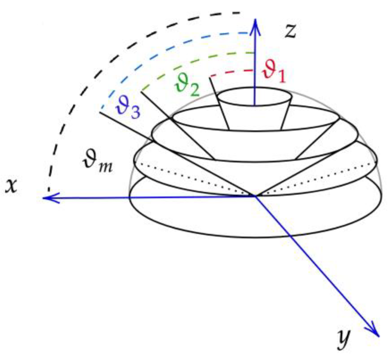
2.1.1. Division of Incident and Reflected Light into Fluxes

Within the framework of the AD algorithm, incoming and outcoming light is divided into m conical fluxes [13], as shown in Figure 1. A cone of light incident on any flat surface will transmit and reflect different amounts of light depending on the angle of departure. To capture this, we introduce the notation for the cosine of an arbitrary angle νc = cos(θ). The function R(ν′, ν) denotes the reflectance in the direction ν for light incident from the direction ν′. The incident light flux, denoted as I+(ν′), and the reflected light flux, denoted as I(ν), can be expressed in the matrix form as:
I ν 1 I ν m = R ν 1 , ν 1 R ν 1 , ν m R ν m , ν 1 R ν m , ν m × I + ν I + ν m
Analytically, the reflected flux can also be calculated as an integral:
I ν = ν 1 ν 2 I + ν R ν , ν 2 ν d ν
where ν1 in ν2 are the boundary angles of the reflected flux I(ν). The total reflected flux for the normal incidence Rc can be determined by the Equation:
R c = 0 1 0 1 δ 1 ν 2 ν R ν , ν 2 ν d ν 2 ν d ν = 0 1 R 1 , ν 2 ν d ν
Figure 1. Division of incident and reflected light into m conical segments.
Algorithms 17 00074 g001

2.1.2. Approximating Reflected Flux Integral Using Quadrature

In the context of the AD algorithm, it is necessary to discretize the integral (Equation (3)) to convert it into matrix form, for which quadrature should be implemented. The integral of the function f(x) on the interval (a, b) with a weight g(x) can be approximated by summing over m points as:
a b f x g x d x i = 1 m f x i w i
The points xi and associated weights wi can be chosen to be either uniformly distributed over the interval or as specific points, such as the zeros of the Legendre polynomials. Using the relation from Equation (4), the integral from Equation (3) can be expressed as:
0 1 R 1 , ν 2 ν d ν i = 1 m 2 ν i w i R i , m
where Ri,m is the reflectance matrix. AD algorithm further divides the integral (expression for the total reflected flux for the normal incidence Rc in Equation (3)) into two parts: the first part on the interval (0, νc), and the second part on the interval (νc, 1], where νc is the cosine of the critical angle:
R c = 0 ν c R 1 , ν 2 ν d ν + ν c 1 R 1 , ν 2 ν d ν
For the first integral, we use the Gaussian quadrature, and the Radau quadrature is used for the second one. The distinction between these two quadrature methods lies in the consideration of endpoints. In Gaussian quadrature, both endpoints are not included, whereas Radau quadrature accounts for only one endpoint. By adopting this approach, we can avoid the potential singularity at ν = 0 in the Gaussian quadrature, while ν = 1 is taken as a quadrature point in the Radau quadrature. In total, we need to find m roots, one for each conical flux: Gaussian and Radau quadratures obtain each half of the quadrature points n = m/2.
In the Radau quadrature, we thus need to find n roots of the following Equation:
R n 1 x i + x i 1 n P n 1 x i = 0
where Pn−1(xi) is the (n − 1)th Legendre polynomial of order zero and Pn−1(xi) denotes the first derivative of the (n − 1)th Legendre polynomial. Since these roots correspond to the integration range from −1 to 1, the appropriate adjustments need to be made for integration angles νc and weights wi when performing integration from νc to 1:
ν i = 1 + ν c 2 1 ν c 2 x i w i = 1 ν c 2 1 x i P n 1 x i 2
Similarly, for the Gaussian quadrature, we need to find n roots of the following Equation:
P n x i = 0
with the adjustments made to accommodate the integration range from 0 to νc:
ν i = ν c 2 1 x i w i = ν c 1 x i 2 P n x i 2 = ν c 1 x i 2 n + 1 2 P n + 1 x i 2

2.1.3. Calculating Scattering Phase Function

Two matrices are constructed, one for forward scattering, denoted as P+, and one for backward scattering, denoted as P. The elements of scattering matrix Pij determine the fraction of light scattered from an incident cone with angle νi into a cone with angle νj and are calculated by averaging the phase function p(νi, νj) over all possible azimuthal angles for fixed angles νi and νj:
P i , j = 1 2 π 0 2 π p ν i ν j + 1 ν i 2 1 ν j 2 cos ϕ d ϕ
The choice between obtaining the forward scattering matrix P+ or the backward scattering matrix P depends on the signs of angles νi and νj. If both angles are either positive or negative, the forward scattering matrix P+ is obtained; otherwise, the backward scattering matrix P is obtained. Furthermore, it is required that the quadrature weighted sum over outgoing angles i for a given incoming angle j adds to 2:
i = 1 m P i , j + + P i , j w i = 2
Matrices P+ and P can be calculated analytically if we utilize the Hanyey–Greenstein scattering phase function (SPF), which is defined as:
p ν , g = 1 2 1 g 2 1 + g 2 + 2 g ν 3 2
where −1 < g < 1 is known as the asymmetry factor. The scattering matrix can be calculated from the following expression:
p ν , g = 1 g 2 π w w + E 0 4 g B w + w ± = 1 + g 2 2 g A ± B
where A = νi νj and B = 1 ν i 2 1 ν j 2 . and E0 (x) denotes an elliptic integral of the second kind.
Alternatively, matrices P+ and P can be calculated through numerical integration:
P i , j ± = 1 2 π 0 2 π p A + B cos z d z
with A and B as defined above. In this case, we employ the Gegenbauer scattering phase function (SPF), given by:
p ν , g , α = 2 α g 1 g 2 2 α 1 + g 2 α 1 g 2 α 1 1 + g 2 2 g ν 1 + α
It has been demonstrated by Engler [20] that when using the trapezoidal rule for numerical integration, an exponential convergence to the accurate scattering matrix elements can be achieved.

2.1.4. Initializing Starting Layer

A very thin layer must be initially simulated with optical thickness dτ, albedo a, and scattering matrices P+ and P. The optical thickness is calculated as τ = (µa + µs)∙d and albedo as a = µs/(µa + µs), where d represents the thickness of the entire layer, and µs and µa are the scattering and absorption coefficients of the layer. Different approaches for initializing the layer exist, with diamond initialization being derived directly from the time-independent, one-dimensional, azimuthally averaged RTE; the details of derivation can be found elsewhere [15]. The initialization involves determining initial matrices using the following matrix relations:
c = diag w M = diag 1 ν A = M I a 2 P + c d τ 2 B = a 2 M P - c d τ 2 G = I + A - B I + A - 1 B 1 R 0 = 2 G B I + A 1 T 0 = 2 G I

2.1.5. Constructing the Entire Layer

Once the reflectance and transmittance matrices of the initial thin layer are obtained, we can proceed to construct the entire layer. However, even before performing any calculations for the initial layer matrices, we must select an appropriate value for the initial layer optical depth. In the literature, two criteria have been proposed for this selection: dτ < 0.01 and dτ < νc For example, when using criterion dτ < 0.01, we can calculate number of doubling steps required:
n d = floor log d 0.01 ν 1 / log 2 + 1
The initial optical depth is then calculated as dτ = τ/(2)nd. with nd defined by Equation (18). To obtain the reflectance and transmittance matrices for the entire layer, the following iterative procedure is performed:
G k = I R k 2 1 R k + 1 = T k G k R k T k + R k T k + 1 = T k G k T k
where k is the number of steps from 0 to nd − 1. The matrices calculated under Equation (17) obtain an index of 0. After that, with each doubling of the layer, the index increases by 1.

2.1.6. Calculating Reflectance and Transmittance

For normal irradiation, the resulting approximation for the reflectance and transmittance is given by:
R n = 0 1 R 1 , ν 2 ν d ν = m 2 2 i = 1 m 2 ν i w i R i , m T n = 0 1 T 1 , ν 2 ν d ν = m 2 2 i = 1 m 2 ν i w i T i , m
while for isotropic irradiation, it is expressed by:
R t = 0 1 2 ν d ν 0 1 R ν , ν 2 ν d ν = m 2 2 2 j = 1 m 2 ν j w j i = 1 m 2 ν i w i R i , j T t = 0 1 2 ν d ν 0 1 T ν , ν 2 ν d ν = m 2 2 2 j = 1 m 2 ν j w j i = 1 m 2 ν i w i T i , j

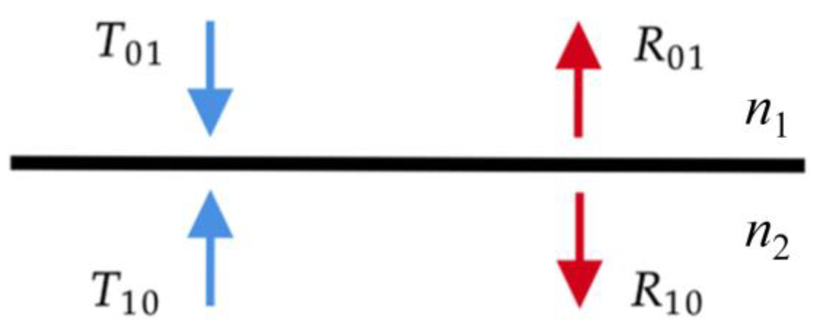
2.1.7. Adding Boundary Layers

Finally, boundary conditions are included as an additional layer when there is a refractive index mismatch between the layer and the surrounding medium. Since the boundary is flat, the Fresnel equations can be used:
r s = n 1 ν 1 n 2 ν 2 n 1 ν 1 + n 2 ν 2 2 r p = n 1 ν 2 n 2 ν 1 n 1 ν 2 + n 2 ν 1 r = r s + r p 2 t = 1 r
As we are dealing with nonpolarized light, we simply average the reflectivities for the s and p polarizations. Before calculating the reflectance and transmittance values, it is necessary to determine the critical angle where total reflection starts:
ν c = 1 n 1 n 2 2
For angles smaller than the critical angle, the cosines outside layer ν1 are calculated from the cosines inside layer ν2 using Snells’s refraction law:
ν 1 = 1 n 2 n 1 1 ν 2 2 2
The boundary matrices are then formulated as follows:
R i , j 01 = r ν 2 δ i , j , ν 2 > ν c δ i , j , ν 2 ν c R 01 = R 10 T 01 = 1 R 01 T 10 = T 01
The reflection r(νi) is the unpolarized Fresnel reflection function, while the Kronecker delta implies matrices R01, R10, T10, and T01 are diagonal, which means that light is specularly reflected at an angle equal to the incident angle [12]. Figure 2 depicts a boundary between medium 0 and 1 with different refraction indices.
The upper boundary is added to the layer, and the corresponding reflectance and transmittance matrices are calculated in the following way:
γ 1 = I R 10 R t 1 T 02 = T t γ 1 T 01 R 20 = T t γ 1 R 10 T t + R t γ 2 = I R t R 10 1 T 20 = T 10 γ 2 T t R 02 = T 10 γ 2 R t T 01
To incorporate the bottom boundary layer, different cases can be specified. In the first case, when the bottom layer is specular, the reflectance matrix RL equals:
R L = R 0 0 0 0 R 0 0 0 0 R 0
where R0 stands for the surface reflectance. In this scenario, only the reflectance matrix at the sample surface is relevant, while the other matrices are 0.
In the second case, when the bottom layer is Lambertian, the reflectance matrix is calculated as follows:
R L = 2 R 0 ν 1 w 1 ν 2 w 2 ν 1 w 1 ν m w m
For the third case, when the bottom layer is assumed to be the same as the external medium, we can employ previously calculated reflectance and transmittance matrices from Equation (25). The reflectance matrices R30 and R03, as well as the transmittance matrices T30 and T03, are determined as follows:
γ 1 = I R 20 R 23 1 T 03 = T 23 γ 1 T 02 R 30 = T 23 γ 1 R 20 T 32 + R 32 γ 2 = I R 23 R 20 1 T 30 = T 20 γ 2 T 32 R 03 = T 20 γ 2 R 23 T 02 + R 02
In the situation where the bottom layer is the same as the external medium, the boundary conditions are identical on the upper and bottom boundaries; thus, we have R01 = R32, R10 = R23, T01 = T32, and T10 = T23. If the bottom layer is specular or Lambertian, then R23 = RL, and only matrix R03 is relevant, as all other matrices R30, T03, and T30 are 0. Once we have obtained all the reflectance and transmittance matrices denoted generically as M, it is necessary to normalize them to ensure they are symmetrical:
M i , j = M i , j 2 ν j w j
After normalization, we can calculate the reflectance and transmittance for normal incidence:
R n 03 = i = 1 m 2 ν i w i R i , m 03 T n 03 = i = 1 m 2 ν i w i T i , m 03
For isotropic irradiance, we can calculate corresponding values of reflectance and transmittance by following Equation (21). Finally, the specular reflectance is determined as follows:
R n s p = i = 1 m 2 ν i w i R i , m 01

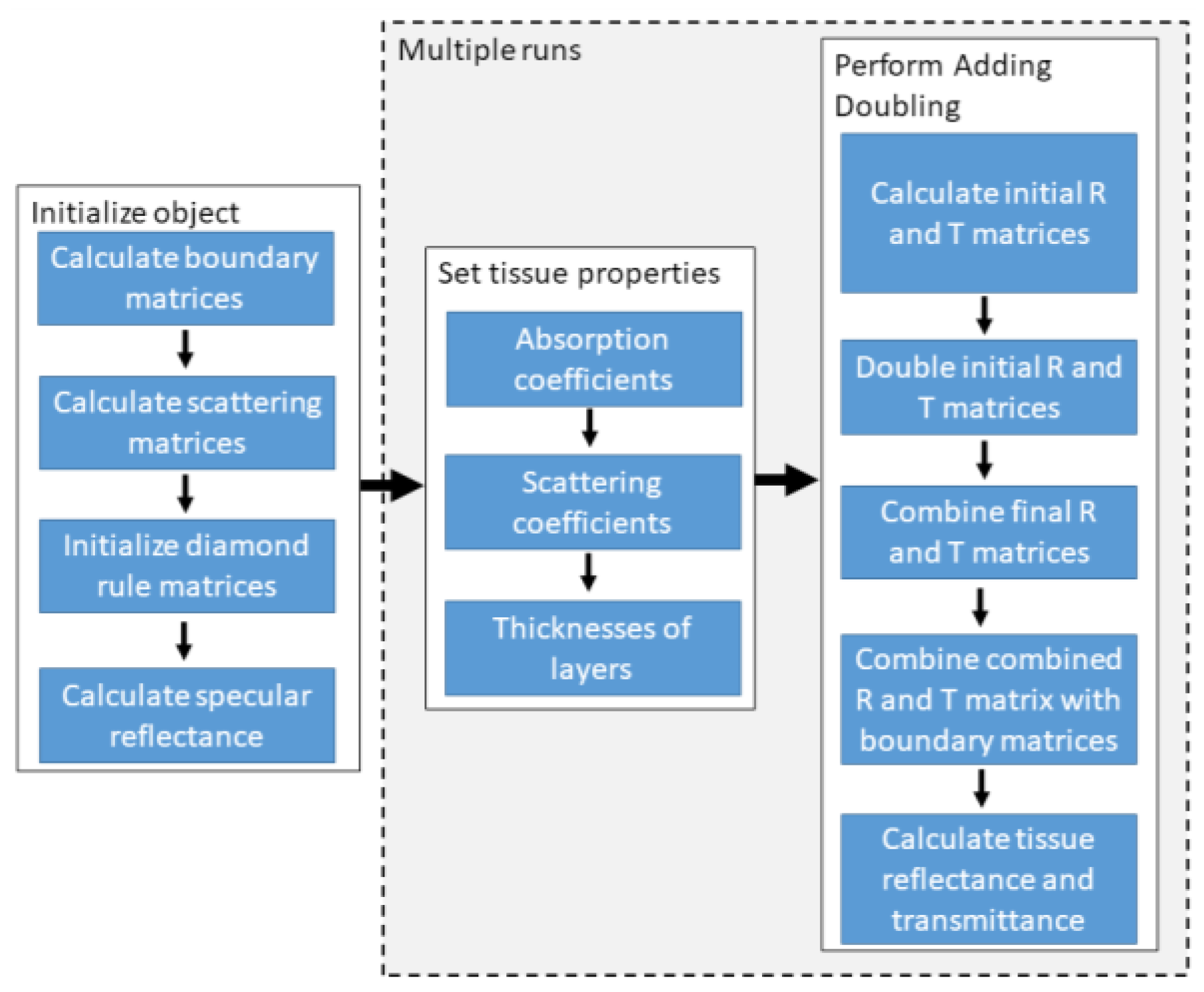
2.2. Implementation of the Adding-Doubling (AD) Algorithm

A GPU-accelerated AD algorithm for single-layer tissue was developed using MATLAB’s parallel toolbox. We utilized the library supporting batched functions, which enabled us to perform parallel calculations of several smaller matrices. Initialization of the CUDA library and running the algorithm on GPU required about 3 s; however, this initialization only needed to be performed once. Subsequent memory allocations would have posed an obstacle, potentially leading to time delays. To tackle this issue, we undertook a comprehensive rearrangement of the code to eliminate the need for for loops and enable the application of the code to larger arrays, specifically optimized for the operations with the previously mentioned library. In this way, we avoided the problem of performance degradation, which would have happened when calculating small matrices on GPU, as the matrix operation times would be comparable to data transfer times between GPU and CPU. Figure 3 shows the flowchart of the CUDA implementation of the GPU-accelerated AD algorithm.
In the following, we will describe the individual parts of the AD1L class. The algorithm is implemented in a custom class AD1L. The class is initialized by calling the constructor AD1L
obj = AD1L(lam, [dtype]);
where lam represents an array of wavelengths with Nl rows. The dtype parameter is optional and specifies the precision used in the algorithm. There are two options: single and double. By default, the precision is set to single as it provides faster computation. An example of the class initialization with double precision is as follows:
A = AD1L(lam, ‘dtype’,’double’);
First, the algorithm is initialized by specifying the properties which remain constant throughout the computation. This includes calculating tissue matrices, such as scattering and reflectance/refraction matrices. The algorithm is initialized by calling the function initPR with the following syntax:
obj = obj.initPR(g, [‘alpha’, alpha], [‘SPFtype’, SPFtype], [‘R0L’, R0L][‘nE’, nE], [‘nS’, nS], [‘m’, m], [‘Nsam’,Nsam])
where g is a matrix of tissue anisotropies at the specified wavelengths lam and samples; the parameters in [] are optional. These optional parameters include:
1. 
alpha—the Gegenbauer scattering phase function (SPF) exponent at the specified wavelengths lam for each sample. It is empty by default;
2. 
SPFtype—the type of SPF to be used. Currently implemented options are Henyey–Greenstein (HG) SPF and Gegenbauer (GB) SPF. To select HG SPF, the parameter value is 0, and to select GB SPF, the parameter value is 1. If GB SPF is selected, the alpha parameter must also be specified;
3. 
R0L—the reflectance of the bottom substrate, ranging between 0 and 1, if it is different from the upper environmental medium. This parameter is used in cases where a sample is placed on top of another thick substrate, such as a support plate. R0L is a matrix with Nl rows corresponding to lam and Ns columns corresponding to the number of samples;
4. 
nE—a column vector of environmental medium refraction indices with Nl values corresponding to lam. By default, the value is set to 1, representing air;
5. 
nS—a column vector of substrate refraction indices with Nl values corresponding to lam. By default, the value is set to 1.4.+;
6. 
m—the number of fluxes (even integer >= 2) used in the algorithm. The default value is 20, as it has been found to provide adequate accuracy for most combinations of optical parameters;
7. 
Nsam—the number of different spectra being calculated. By default, it is set to 1, meaning that only one set of different wavelengths is considered.
An example of initializing the algorithm, providing g for Gegenbauer SPF and 20 fluxes, can be performed as follows:
A.initPR(g,’SPFtype’,1,’alpha’,alpha,’m’,20);
where g is a column vector of Nl anisotropy factors, alpha is a column vector of Nl GB SPF exponents, and m is the number of fluxes.
The variable properties of the tissues are set by calling the setOP method. The calling syntax is
obj = obj.setOP(muA, muS, d)
where muA and muS represent the matrices of absorption and scattering coefficients in units of [1/cm], and d is the layer thickness in units of [cm]. The dimensions of muA and muS are Nl rows and Ns columns, while d has Ns values, one for each sample.
An example of calling this method is
A.setOP(muAar,muSar,d);
Finally, the solveAD is called to calculate the reflectance and transmittance values at the specified wavelengths. The calling syntax is
obj = obj.solveAD()
Although this method does not directly return any values, it stores the results in the class properties. Currently, only normal incidence of the illumination and complete diffuse reflectance and transmittance (e.g., all radiation in the exit hemispheres, two solid angles) are supported.
The results can be retrieved through the following properties:
-
obj.Rn—2 diffuse reflectance;
-
obj.Tn—2 transmittance;
-
obj.Rsp—specular reflectance.
An example of retrieving all these parameters in a MATLAB environment is:
[A.Rn, A.Tn, A.Rsp]

2.3. Single-Layer AD Model Simulations

To evaluate the accuracy and computational speed of the AD1L algorithm, a comparison was made with layered MC results. The MC simulation was conducted using CUDA MCML software [21], which provided sufficient computational speed for the calculations. To achieve acceptable accuracy, 107 photons were simulated. The simulated single layer had fixed properties, including a thickness d of 1 cm, a sample refraction index nS of 1.4, and an environmental medium refraction index nE of 1, corresponding to air. The environmental medium was present on both sides of the layer.
To cover a range of optical properties similar to the SiliGlass tissue phantoms prepared in our lab, various absorption coefficients muA (0.1, 0.5, and 1.0/cm) and scattering coefficients muS (25, 50, 100, and 150/cm) were used. The computation was carried out using a single GeForce GTX TITAN X graphic card (Nvidia, Santa Clara, CA, USA).

2.4. Inverse Adding-Doubling (IAD) Solution

In addition to the forward problem, the GPU AD algorithm demonstrated utility in solving the inverse scattering problem. The human skin model used for this purpose consisted of two layers: epidermis and dermis (Figure 4). The epidermis and dermis are characterized by various optical parameters, which are discussed in more detail in Appendix A. The diamond initialization was used to simulate an initial thin skin layer, and the incident and reflected light were divided into 20 fluxes to ensure accurate results. To perform non-linear least-squares fitting, the Levenberg–Marquardt (LM) algorithm (Appendix B) was adopted on the GPU; the maximum number of iterations for the LM algorithm was limited to 200. A large batch of HSI reflectance spectra in the range of 430–750 nm with a step of 5 nm was fitted at once, enabling a rapid solution of the inverse scattering problem. The total number of fitting parameters was 11; however, only 6 were considered free variables: (a) volume fraction of melanin, fm, (b) volume fraction of deoxyhemoglobin, fHb, (c) volume fraction of oxyhemoglobin, fHbO2, (d) scattering factor a, where a = µs (λ = 500 nm), (e) scattering power, b, and (f) fraction of Rayleigh scattering, fRay. Among these free parameters, (a) and (d–f) were fitted for the epidermis, and (b–f) were fitted for the dermis. Several fixed parameters were also defined: (a) volume fraction of bilirubin, fbrub, was set to 0.01, (b) volume fraction of reduced cytochrome oxidase, fCO, was fixed to 0.01; (c) volume fraction of oxidized cytochrome oxidase, fCOO2, was set to 0.01, (d) epidermis thickness, depi, was fixed at 0.2 mm, and (e) dermis thickness, dder, was set to 1 cm. While the LM algorithm allowed the fitting of all parameters, the above parameters were fixed to prevent crosstalk between different sets of parameters and, therefore, improve the robustness of the inverse problem-solving process.
To test the reliability and robustness of the GPU LM algorithm, a healthy participant’s forearm was imaged with the HSI-integrated imaging system [22] before, during, and after applying a blood pressure cuff. Prior to cuff application, a steady-state image was acquired. The cuff was then inflated to about 200 mmHg to obstruct the blood flow completely, and the image was recorded three minutes after the initial inflation. Subsequently, the cuff was deflated, and one minute later, another image was captured. Hyperspectral images were acquired and processed as described in detail in our previous publications [22,23,24].

3. Results

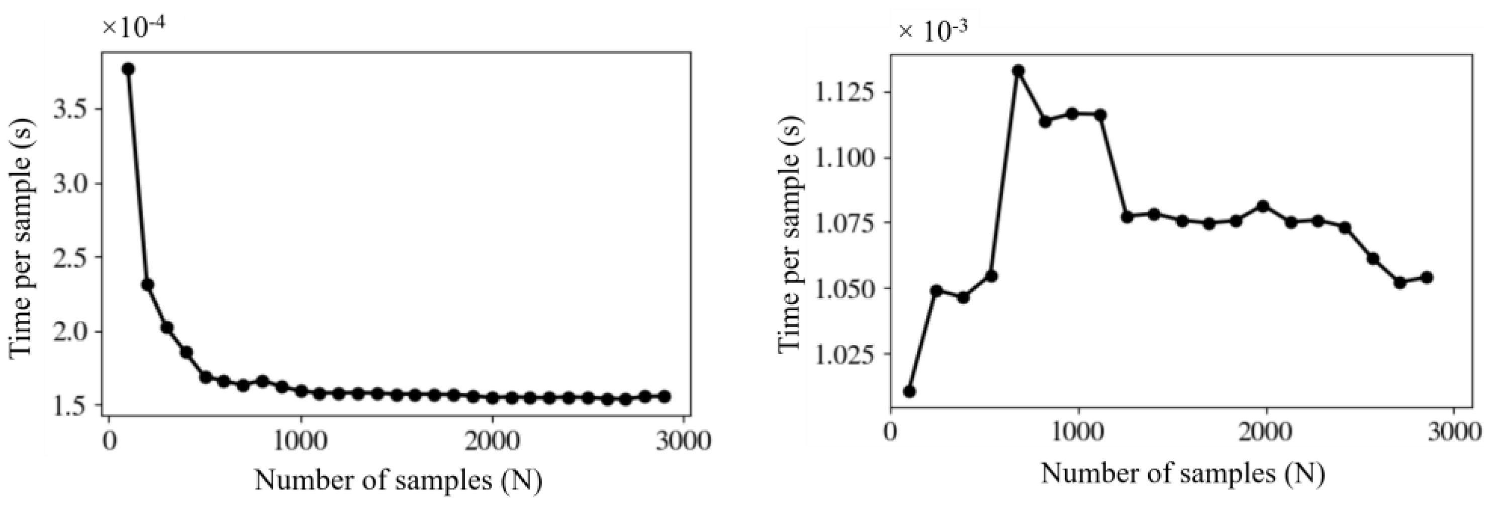
3.1. Comparison between the Performance of GPU-Accelerated AD and CPU AD Algorithms

In the preliminary step, we compared GPU-accelerated AD and CPU AD algorithms. By repeatedly executing each algorithm 1000 times, we derived average times of solveAD as representative values, thereby minimizing the impact of external factors. For fixed values of absorption coefficient muA = 0.1/cm, scattering coefficient muS = 25/cm, and a number of fluxes m = 20, we found that the GPU-accelerated AD algorithm was roughly seven times faster than the CPU AD algorithm (time per sample of 1.5 × 10⁻⁴ s vs. 1.1 × 10⁻³ s) (Figure 5). As shown in Figure 5, time per sample stabilized at around 1000 samples for GPU, while time per sample for CPU changed only marginally with the number of samples.

3.2. Comparison between Single and Double Precision for Single-Layer AD Model Simulations

We conducted a comparative analysis of reflectance and transmittance calculations using both single and double precision. The testing involved all possible combinations of absorption coefficients (μa = 0.1, 0.5, 1.0 cm−1) and scattering coefficients (μs = 25, 50, 100, 150 cm−1) at m = 20. The relative difference between the single and double precision results for reflectance ranged from 2 × 10⁻⁷ to 6 × 10⁻⁵; the highest discrepancy occurred with the combination of the highest scattering coefficient and the smallest absorption coefficient. For transmittance, the differences between the single and double precision results were slightly higher, between 2 × 10⁻⁶ and 5 × 10⁻⁴, the worst agreement corresponding again to the highest scattering and lowest absorption coefficients. However, these discrepancies are considerably smaller than the typical noise amplitude encountered in experimental spectra, which usually falls within the range of 1%.
In terms of computation speed, the single precision computations were, on average, 4.3 times faster compared to double precision when considering the above set of optical parameters. In addition to the faster computation, the advantage of using single precision is that it also has two times lower memory requirements, facilitating the upload of larger datasets to the GPU memory.

3.3. Single-Layer AD Model Simulations

We compared the AD algorithm with MC separately for the HG SPF and GB SPF. As the results were similar for both SPFs, we are presenting the results solely for the GB SPF with the exponent αGB set at 1.051 and factor of anisotropy g at 0.851. Our evaluation focused on different numbers of fluxes, specifically m = 8, 12, 16, and 20.
Table 1 shows results for reflectance and transmittance, obtained using the CUDA MCML software, while Table 2 and Table 3 exhibit results obtained using the AD1L algorithm with single precision. A comparison between MCML and AD1L reveals that perfect agreement was reached for m = 20, though adequate accuracy was obtained for m = 16.
To assess the computational speed of the GPU-accelerated AD1L algorithm, we considered different simultaneous numbers of threads: 100, 1000, and 3000. Table 4 presents the computation times for the MC method per single optical properties set, whereas Table 5 and Table 6 present the corresponding results for the AD1L algorithm using the GB SPF for the number of examined fluxes m = 20 and m = 16, respectively. Comparing the MC method to the AD1L algorithm, we found that at m = 16 and a thread count of N = 3000, the speed-up ranged from 5333 to 40,556 times (Table 7). The computation times did not vary between the two SPFs since the number of elements in the array was the same. The optimal number of threads for the AD1L algorithm was around 3000; larger batches of threads did not considerably enhance computational speed.

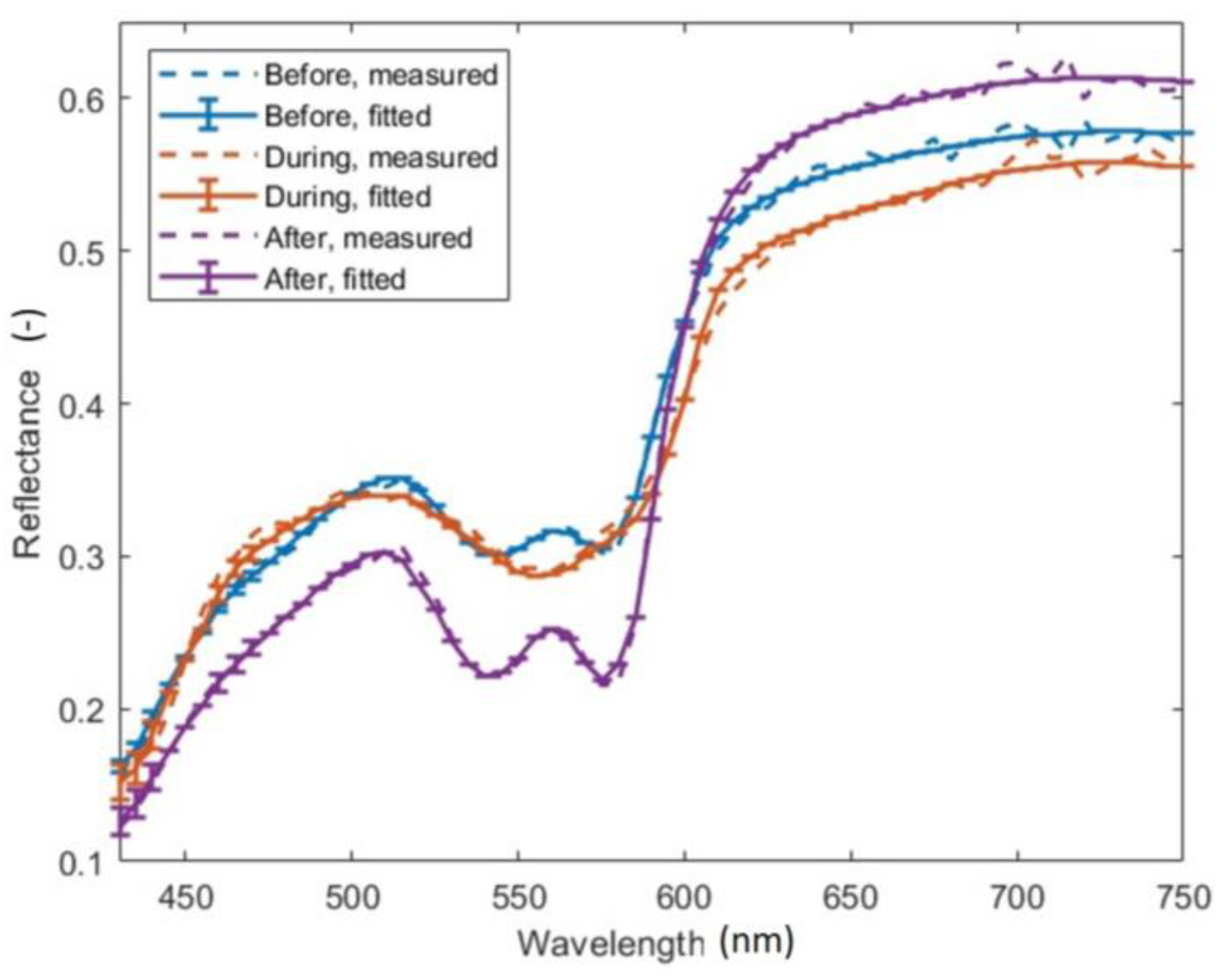
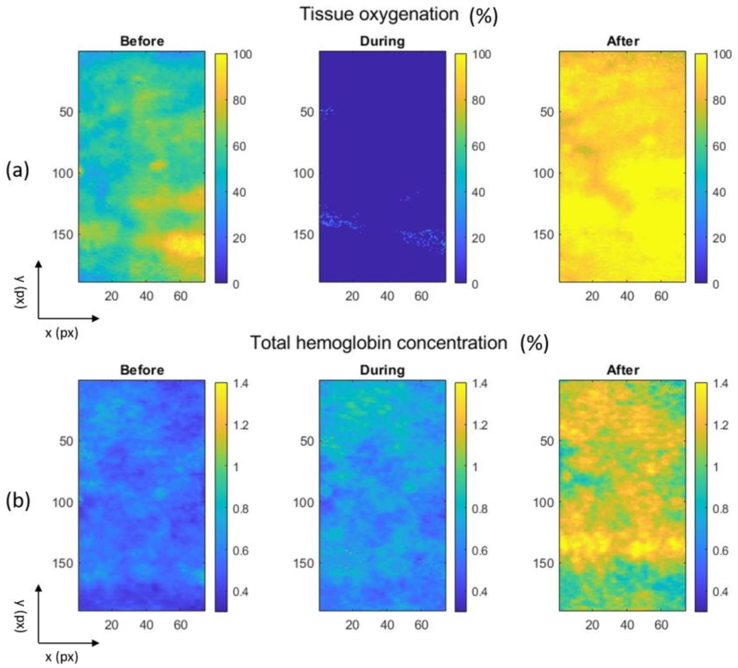
3.4. Inverse Adding-Doubling (IAD) Solution: Arterial Occlusion Test

Results obtained with a GPU-accelerated LM algorithm are shown alongside measured data in Figure 6. Here, reflectance spectra of skin before, during, and after a cuff test are presented for a single spatial data point in a curvature-corrected hyperspectral image [25]. Upon examining the calculated spectra, we observed excellent agreement with the measured data across the entire spectral range of 430–750 nm. However, minor deviations can be spotted near 700 nm due to slight wiggles in the measured spectra. To assess the goodness of fit, we calculated the reduced χ2 value for each spatial data point; the computed data yielded reduced χ2 ranging from 10−5–10−4. In terms of computational efficiency, it took approximately 5 min to process a 220 × 100 × 61 image (x-axis × y-axis × spectral-axis).
Figure 7 shows colormaps extracted from the hyperspectral images by the inverse AD algorithm, depicting tissue oxygenation, calculated as the ratio of fHbO2 to the sum of fHb and fHbO2 multiplied by 100%, and the total hemoglobin concentration, calculated as a sum of fHb and fHbO2 multiplied by 100%. These colormaps capture the conditions before, during, and after a cuff test. Upon analyzing Figure 7a, we observe that tissue oxygenation is visibly reduced during the cuff test, coinciding with the obstruction of blood flow when a blood-pressure cuff is inflated to around 200 mmHg. Additionally, we can discern from Figure 7b a slight increase in the total hemoglobin concentration throughout the entire experiment. Conversely, tissue oxygenation reaches its peak approximately 3 min after deflating the blood-pressure cuff, indicating rapid tissue reoxygenation following the vascular obstruction.
To quantify our observations from the colormaps, we present mean values and standard deviations of tissue oxygenation and the total hemoglobin concentration before, during, and after the cuff test in Table 8. These numerical findings substantiate the conclusions drawn from the visual examination of the colormaps in Figure 5 and also corroborate data reported by Verdel et al. [26].

4. Discussion

Our study has demonstrated that the AD algorithm matches the accuracy of the MC method while also being versatile and compatible with implementation on GPUs. The computational speed-up achieved by the GPU-accelerated AD algorithm when compared to the GPU MC method, ranges from about 5000 to 40,000 times faster. This remarkable improvement in computational efficiency allows for the entire hyperspectral image to be analyzed within minutes. While the MC method excels in capturing intricate photon interactions, its computational demands are often prohibitive for large-scale simulations. In contrast, the AD algorithm serves as a more efficient alternative, offering an analytical solution that strikes a balance between accuracy and computational efficiency.
Based on our study results, we can conclude that a GPU-accelerated two-layer IAD provides an acceptably accurate, fast, and reliable approach for solving inverse scattering problems and extracting important tissue properties, such as scattering properties and chromophore concentrations. Our calculated skin reflectance values align closely with the measurements taken before, during, and after the cuff test. Additionally, the obtained tissue properties using the IAD approach effectively reflect the changes in tissue physiology.
In recent years, the use of GPUs has advanced computational efficiency and accelerated processing capabilities. In our study, we specifically focused on implementing the AD algorithm on GPUs to enhance computational speed further. Additionally, we combined the AD and LM algorithms on the GPU platform to extract object parameters from optical spectral data effectively. By harnessing the power of GPUs, we aimed to achieve improvements in the computational speed of AD calculations. This integration of GPU technology with the AD algorithm holds the potential to advance our understanding of light transport in biological tissues and can pave the way for more efficient simulations and clinical applications, either in HSI [27] or related biomedical optical applications [28,29].
In our previous publication, we reported a GPU implementation of the diffuse approximation algorithm for analyzing hyperspectral images of skin [30]. Although this algorithm proved to be sufficiently fast in providing extracted tissue parameter maps in (almost) real-time, its primary limitation is that it is an approximation only, and therefore, the resulting maps differ from the true values. On the other hand, the AD algorithm is as accurate as the MC algorithm; thus, the extracted tissue properties correspond to the true values, as demonstrated in our recent publication [31]. Although real-time image processing has not been achieved yet, we believe that by reducing the number of the analyzed wavelengths, further optimizing the algorithm, and implementing it in more computationally efficient programming languages, we can attain real-time image analysis. This advancement would make HSI even more attractive for clinical applications.
Our approach has an obvious limitation in that it operates under assumptions outlined by Prahl et al. [13], including the absence of time dependence, a geometric model comprising uniform layers of finite thickness extended infinitely parallel to the surface, uniform scattering and absorbing properties within tissue layers, and uniform illumination by collimated or diffuse light. While these assumptions do not contradict the application of GPU AD to HSI, it may be necessary to resort to the MC method in more complex cases when, for example, a beam would be spreading from a finite source [32].
An obvious extension of our AD approach involves transitioning from MATLAB to Python. We have already begun exploring this direction, and preliminary results indicate an additional computational speed-up ranging from a factor of 3 to 10 when comparing GPU AD (Python) to GPU AD (MATLAB). Furthermore, the GPU AD method itself has the potential to accelerate machine learning techniques (ML) in spectral image analysis by providing data for the training process. In contrast to the MC algorithm, the AD algorithm can generate large training datasets in significantly shorter times, facilitating faster optimizations of ML tools.
Through thorough development and testing, we have successfully implemented the GPU-based AD algorithm, which offers an analytical solution for the RTE. Our research has demonstrated the GPU AD algorithm’s significant speedup over the GPU MC method while maintaining a high level of accuracy. We have also shown that the GPU AD algorithm can be used to extract tissue parameters from optical spectral data of human skin under various hemodynamic conditions using the Levenberg–Marquardt inverse algorithm. The GPU AD algorithm can process large spectral images within minutes, surpassing the performance of other RTE solutions. Therefore, it has the potential for real-time processing of spectral imaging in the clinical environment.

Author Contributions

Conceptualization, R.H. and M.M.; methodology, R.H. and M.M.; software, M.M.; validation, M.M.; formal analysis, R.H. and M.M.; investigation, R.H.; resources, M.M.; data curation, M.M.; writing—original draft preparation, R.H.; writing—review and editing, R.H. and M.M.; visualization, M.M.; supervision, R.H. and M.M.; project administration, R.H. and M.M.; funding acquisition, M.M. All authors have read and agreed to the published version of the manuscript.

Funding

This research was funded by the Slovenian Research and Innovation Agency, grant numbers P1-0389 and J3-3083.

Institutional Review Board Statement

The study was conducted in accordance with the Declaration of Helsinki and approved by the Medical Ethics Committee of the Republic of Slovenia (protocol code 66/01/17 and date of approval 25 May 2017).

Informed Consent Statement

Informed consent was obtained from all subjects involved in the study.

Data Availability Statement

Data and the MATLAB implementation of the algorithms are available upon reasonable request to the corresponding author.

Acknowledgments

The authors wish to thank Anej Sterle for running the simulations.

Conflicts of Interest

The authors declare no conflicts of interest.

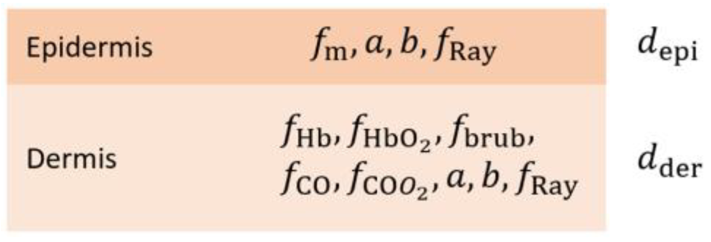
Appendix A. Optical Parameters of Epidermis and Dermis

Skin, the largest organ in the human body, covers a total surface area of approximately 1.6–1.8 m2 and weighs around 8% of the total body weight in adults [33]. It consists of two main layers—the epidermis and dermis, which rest on the subcutaneous fat layer, called the subcutis; the epidermis (approximately 100–150 μm) is thinner than the dermis (approximately 2–4 mm), which contains structural proteins such as collagen and elastin [33]. When exposed to ultraviolet (UV), visible (VIS), and near-infrared (NIR) radiation, human skin exhibits distinct photobiological responses, which strongly depend on, among others, melanin, oxygenated and deoxygenated blood particles, and water.
In the model of the epidermis and the dermis, presented in Figure 4, we considered the following six optical parameters as free variables, which we briefly outline for the epidermis and the dermis separately.

Appendix A.1. Epidermis

The volume fraction of melanin fm measures the concentration of melanin pigment in the epidermis. Measuring fm can provide insights into various skin conditions, such as hyperpigmentation, hypopigmentation, and melanoma.

Appendix A.2. Epidermis and Dermis

Scattering factor a = µs (λ = 500 nm) quantifies the scattering properties of tissue at a specific wavelength, usually 500 nm. It measures how light scatters within tissue due to interactions with cellular and subcellular structures.
Scattering power b is a parameter that characterizes the scattering intensity of the tissue. It provides insights into the size and density of scattering particles within the tissue, affecting the degree of light dispersion.
Fraction of Rayleigh scattering fRay refers to the scattering caused by small molecules or particles compared to other forms of scattering. It is significant in studying tissue composition and structure, as it provides information about the molecular and chemical composition of the tissue.

Appendix A.3. Dermis

The volume fraction of deoxyhemoglobin fHb signifies the concentration of oxygen-poor hemoglobin in tissue and serves as an indicator of tissue oxygenation. Monitoring changes in fHb is valuable for studying conditions like hypoxia, ischemia, and vascular disorders.
The volume fraction of oxyhemoglobin fHbO2 represents the concentration of oxygen-rich hemoglobin in tissue and provides information about tissue oxygenation. Monitoring changes in fHbO2 is particularly relevant in studying tissue response to interventions, such as in oncology treatments or surgical procedures.

Appendix A.4. Other Parameters

The following five other parameters (four in the dermis and one in the epidermis) were treated as fixed variables: fbrub—volume fraction of bilirubin; fCO—volume fraction of reduced cytochrome oxidase; fCOO2—volume fraction of oxidized cytochrome oxidase; depi—epidermis thickness; dder—dermis thickness. The volume fraction of bilirubin fbrub measures the concentration of bilirubin, a yellow pigment derived from the breakdown of heme in red blood cells; elevated levels of bilirubin can indicate liver dysfunction. An increase in the volume fraction of reduced cytochrome oxidase fCO cytochrome oxidase generally indicates a higher level of cellular respiration and oxygen consumption, while the presence of oxidized cytochrome oxidase fCOO2 usually indicates a lower metabolic activity and reduced oxygen consumption.

Appendix B. Levenberg–Marquardt Algorithm

The Levenberg–Marquardt (LM) algorithm is a well-known tool for solving nonlinear least squares problems [34,35,36,37]. LM has been implemented as a MATLAB Class for multithread GPU fitting of spectral images. Matlab Class consists of multiple properties and methods, which are described below.

Appendix B.1. Initialization

The class is initialized by calling the class constructor:
LM = Fit_X_(lam,img,[dtype]);
where _X_ represents the tissue light transport method to be fitted. The necessary parameters are:
  • lam—vector of wavelengths (Nl × 1);
  • img—spectral image (Nx × Ny × Nl).
  • Where Nl is the number of wavelengths, and Nx and Ny are the numbers of image pixels in x- and y-directions.
The optional parameter is as follows:
  • dtype—the datatype used for the computation. It can be either ‘single’ for the single precision or ‘double’ for the double precision.
The initialization stores image data and wavelengths in the class properties.

Appendix B.2. Algorithm Setup

The algorithm is set by calling the InitLM method; it is the main function where all parameters of the algorithms are set:
LM.InitLM(pimg0,[options])
The necessary parameters are as follows:
pimg0—the initial parameters for the model function (Nx × Ny × Npar).
Optional parameters are as follows:
  • dp—fractional increment of parameters p for numerical derivatives (Npar × 1). Default: 0.005. Additional info:
    • dp(j) > 0 central differences calculated;
    • dp(j) < 0 one-sided ‘backwards’ differences calculated;
    • dp(j) = 0 sets corresponding partials to zero, i.e., holds p(j) fixed;
  • p_min—lower bounds for parameter values (Npar × 1). Default values depend on the tissue type;
  • p_max—upper bounds for parameter values (Npar × 1). Default values depend on the tissue type;
  • weight—weight matrices (Nl × Nl) or a scalar weight value; weight must be non-negative. For more information about weights, see [36]. Default value: 1;
  • eps1—convergence in the gradient. Default value: 1 × 10⁻⁴;
  • eps2—convergence in parameters. Default value: 1 × 10⁻⁴;
  • eps3—convergence in χ2. Default value: 1 × 10⁻⁴;
  • eps4—λlm update criterion. Default value: 1 × 10⁻³;
  • MaxIter—maximum number of iterations. Default value: 200;
  • L0—initial lambda value. Default value: 1 × 10⁻³;
  • Lu—lambda increase multiplicator. Default value: 1.5;
  • Ld—lambda decrease divisor. Default value: 5;
  • Update_Type LM lambda update method. Parameter values: 1 = Levenberg–Marquardt lambda update (default), 2 = Quadratic update, 3 = Nielsen’s lambda update equations, 4 = geodesic acceleration;
  • epsJtWJ—the minimum allowed value of the Levenberg-Marquardt damping term (Update_Type = 1). Default value: 1 × 10⁻³;
  • dg—geodesic acceleration FD step. Default value: 0.1;
  • galpha—geodesic acceleration acceptance criterion. Default value: 0.75;
  • Broyden—Broyden’s rank 1 update for Jacobian, preventing the calculation of finite differences, 1 = use, 0 = do not use rank 1 approximation. Default value: 1;
  • lambdaMax—maximum dumping parameter lambda. Default value: 10;
  • muPenTer—penalty term for the nearest neighbor’s initial coefficient. Set to 0 if no term penalty is required. Default value: 1;
  • Nsit—number of spectra fitted simultaneously. Default value: 10;
  • Verbose—Display messages during execution. Parameter values: 0 = no messages, 1 = messages. Default value: 1
The constraint (i.e., muPenTer) takes care to penalize individual parameter values that are significantly different from the parameter values in the neighbor spatial points.

Appendix B.3. Running

The optimization is started by calling the RunFit method:
LM.RunFit;
The method starts an iterative process of finding the optimal parameters, minimizing the input data—model values. The final results are stored in the class properties.

Appendix B.4. Output

The output variables are stored in the class properties and can be accessed directly by calling:
LM.[variable]
The output variables are:
  • pimgOut—fitted parameters (Nx × Ny × Npar);
  • imgOut—fitted image (Nx × Ny × Nl);
  • redX2—reduced χ2 (Nx × Ny × 1);
  • sigma_p—asymptotic standard parameter errors (Nx × Ny × Npar);
  • sigma_y—standard error of the fit (Nx × Ny × Nl);
  • corr_p—parameter correlation matrix (Nx × Ny × Npar × Npar);
  • R_sq—coefficient of multiple determination (Nx × Ny × 1);
  • iterOut—matrix of iterations needed in each image point to stop fitting.

References

  1. Stokes, G.G., IV. On the intensity of the light reflected from or transmitted through a pile of plates. Proc. R. Soc. Lond. 1862, 11, 545–556. [Google Scholar] [CrossRef]
  2. van de Hulst, H.C.; Christoffel, H. A New Look at Multiple Scattering; NASA Institute for Space Studies: New York, NY, USA, 1962. [Google Scholar]
  3. Liu, Q.; Weng, F. Advanced Doubling–Adding Method for Radiative Transfer in Planetary Atmospheres. J. Atmos. Sci. 2006, 63, 3459–3465. [Google Scholar] [CrossRef]
  4. Zhang, Z.; Yang, P.; Kattawar, G.; Huang, H.-L.; Greenwald, T.; Li, J.; Baum, B.A.; Zhou, D.K.; Hu, Y. A fast infrared radiative transfer model based on the adding–doubling method for hyperspectral remote-sensing applications. J. Quant. Spectrosc. Radiat. Transf. 2007, 105, 243–263. [Google Scholar] [CrossRef]
  5. Mukai, S.; Sano, I.; Nakata, M. Improved Algorithms for Remote Sensing-Based Aerosol Retrieval during Extreme Biomass Burning Events. Atmosphere 2021, 12, 403. [Google Scholar] [CrossRef]
  6. Leyre, S.; Cappelle, J.; Durinck, G.; Abass, A.; Hofkens, J.; Deconinck, G.; Hanselaer, P. The use of the adding-doubling method for the optical optimization of planar luminescent down shifting layers for solar cells. Opt. Express 2014, 22, A765. [Google Scholar] [CrossRef] [PubMed]
  7. Pickering, J.W.; Prahl, S.A.; Van Wieringen, N.; Beek, J.F.; Sterenborg, H.J.C.M.; Van Gemert, M.J.C. Double-integrating-sphere system for measuring the optical properties of tissue. Appl. Opt. 1993, 32, 399. [Google Scholar] [CrossRef] [PubMed]
  8. Lemaillet, P.; Cooksey, C.C.; Hwang, J.; Wabnitz, H.; Grosenick, D.; Yang, L.; Allen, D.W. Correction of an adding-doubling inversion algorithm for the measurement of the optical parameters of turbid media. Biomed. Opt. Express 2018, 9, 55. [Google Scholar] [CrossRef] [PubMed]
  9. Sun, B.; Gao, C.; Spurr, R. Scalar thermal radiation using the adding-doubling method. Opt. Express 2022, 30, 30075. [Google Scholar] [CrossRef] [PubMed]
  10. Liu, X.; Wu, Y. Monte-Carlo optical model coupled with Inverse Adding-Doubling for Building Integrated Photovoltaic smart window design and characterisation. Sol. Energy Mater. Sol. Cells 2021, 223, 110972. [Google Scholar] [CrossRef]
  11. Calvin, O.W.; Ganapol, B.D.; Borrelli, R.A. Introduction of the Adding and Doubling Method for Solving Bateman Equations for Nuclear Fuel Depletion. Nucl. Sci. Eng. 2023, 197, 558–588. [Google Scholar] [CrossRef]
  12. Prahl, S.A. The Adding-Doubling Method. In Optical-Thermal Response of Laser-Irradiated Tissue; Welch, A.J., Van Gemert, M.J.C., Eds.; Springer: Boston, MA, USA, 1995; pp. 101–129. [Google Scholar] [CrossRef]
  13. Prahl, S.A.; Van Gemert, M.J.C.; Welch, A.J. Determining the optical properties of turbid media by using the adding–doubling method. Appl. Opt. 1993, 32, 559. [Google Scholar] [CrossRef]
  14. Prahl, S.A. A Monte Carlo model of light propagation in tissue. In Proceedings of the Institutes for Advanced Optical Technologies, Berlin, Germany, 10 January 1989; Mueller, G.J., Sliney, D.H., Potter, R.F., Eds.; p. 1030509. [Google Scholar] [CrossRef]
  15. Wang, C.-Y.; Kao, T.-C.; Chen, Y.-F.; Su, W.-W.; Shen, H.-J.; Sung, K.-B. Validation of an Inverse Fitting Method of Diffuse Reflectance Spectroscopy to Quantify Multi-Layered Skin Optical Properties. Photonics 2019, 6, 61. [Google Scholar] [CrossRef]
  16. Després, P.; Jia, X. A review of GPU-based medical image reconstruction. Phys. Medica 2017, 42, 76–92. [Google Scholar] [CrossRef] [PubMed]
  17. Kalaiselvi, T.; Sriramakrishnan, P.; Somasundaram, K. Survey of using GPU CUDA programming model in medical image analysis. Inform. Med. Unlocked 2017, 9, 133–144. [Google Scholar] [CrossRef]
  18. Smistad, E.; Falch, T.L.; Bozorgi, M.; Elster, A.C.; Lindseth, F. Medical image segmentation on GPUs—A comprehensive review. Med. Image Anal. 2015, 20, 1–18. [Google Scholar] [CrossRef]
  19. Alcaín, E.; Fernández, P.R.; Nieto, R.; Montemayor, A.S.; Vilas, J.; Galiana-Bordera, A.; Martinez-Girones, P.M.; Prieto-De-La-Lastra, C.; Rodriguez-Vila, B.; Bonet, M.; et al. Hardware Architectures for Real-Time Medical Imaging. Electronics 2021, 10, 3118. [Google Scholar] [CrossRef]
  20. Engler, H. Computation of Scattering Kernels in Radiative Transfer. arxiv 2015. [Google Scholar] [CrossRef]
  21. Alerstam, E.; Svensson, T.; Andersson-Engels, S. Parallel computing with graphics processing units for high-speed Monte Carlo simulation of photon migration. J. Biomed. Opt. 2008, 13, 060504. [Google Scholar] [CrossRef]
  22. Stergar, J.; Hren, R.; Milanič, M. Design and Validation of a Custom-Made Laboratory Hyperspectral Imaging System for Biomedical Applications Using a Broadband LED Light Source. Sensors 2022, 22, 6274. [Google Scholar] [CrossRef]
  23. Rogelj, L.; Simončič, U.; Tomanič, T.; Jezeršek, M.; Pavlovčič, U.; Stergar, J.; Milanič, M. Effect of curvature correction on parameters extracted from hyperspectral images. J. Biomed. Opt. 2021, 26, 096003. [Google Scholar] [CrossRef]
  24. Rogelj, L.; Dolenec, R.; Tomšič, M.V.; Laistler, E.; Simončič, U.; Milanič, M.; Hren, R. Anatomically Accurate, High-Resolution Modeling of the Human Index Finger Using In Vivo Magnetic Resonance Imaging. Tomography 2022, 8, 2347–2359. [Google Scholar] [CrossRef] [PubMed]
  25. Rogelj, L.; Pavlovčič, U.; Stergar, J.; Jezeršek, M.; Simončič, U.; Milanič, M. Curvature and height corrections of hyperspectral images using built-in 3D laser profilometry. Appl. Opt. 2019, 58, 9002. [Google Scholar] [CrossRef]
  26. Verdel, N.; Marin, A.; Milanič, M.; Majaron, B. Physiological and structural characterization of human skin in vivo using combined photothermal radiometry and diffuse reflectance spectroscopy. Biomed. Opt. Express 2019, 10, 944. [Google Scholar] [CrossRef] [PubMed]
  27. Hren, R.; Sersa, G.; Simoncic, U.; Milanic, M. Imaging perfusion changes in oncological clinical applications by hyperspectral imaging: A literature review. Radiol. Oncol. 2022, 56, 420–429. [Google Scholar] [CrossRef] [PubMed]
  28. Hren, R.; Sersa, G.; Simoncic, U.; Milanic, M. Imaging microvascular changes in nonocular oncological clinical applications by optical coherence tomography angiography: A literature review. Radiol. Oncol. 2023, 57, 411–418. [Google Scholar] [CrossRef] [PubMed]
  29. Marin, A.; Hren, R.; Milanič, M. Pulsed Photothermal Radiometric Depth Profiling of Bruises by 532 nm and 1064 nm Lasers. Sensors 2023, 23, 2196. [Google Scholar] [CrossRef] [PubMed]
  30. Bjorgan, A.; Milanic, M.; Randeberg, L.L. Estimation of skin optical parameters for real-time hyperspectral imaging applications. J. Biomed. Opt. 2014, 19, 066003. [Google Scholar] [CrossRef] [PubMed]
  31. Tomanič, T.; Rogelj, L.; Milanič, M. Robustness of diffuse reflectance spectra analysis by inverse adding doubling algorithm. Biomed. Opt. Express 2022, 13, 921. [Google Scholar] [CrossRef]
  32. Klanecek, Z.; Hren, R.; Simončič, U.; Muc, B.T.; Lukač, M.; Milanič, M. Finite Element Method (FEM) Modeling of Laser-Tissue Interaction during Hair Removal. Appl. Sci. 2023, 13, 8553. [Google Scholar] [CrossRef]
  33. Young, A.R. Chromophores in human skin. Phys. Med. Biol. 1997, 42, 789–802. [Google Scholar] [CrossRef]
  34. Hren, R.; Stroink, G. Application of the surface harmonic expansions for modeling the human torso. IEEE Trans. Biomed. Eng. 1995, 42, 521–524. [Google Scholar] [CrossRef]
  35. Hren, R.; Zhang, X.; Stroink, G. Comparison between electrocardiographic and magnetocardiographic inverse solutions using the boundary element method. Med. Biol. Eng. Comput. 1996, 34, 110–114. [Google Scholar] [CrossRef] [PubMed]
  36. Gavin, H.P. The Levenberg-Marquardt Algorithm for Nonlinear Least Squares Curve-Fitting Problems. 27 November 2022. Available online: https://people.duke.edu/~hpgavin/ExperimentalSystems/lm.pdf (accessed on 3 February 2024).
  37. Du, Y.-C.; Stephanus, A. Levenberg-Marquardt Neural Network Algorithm for Degree of Arteriovenous Fistula Stenosis Classification Using a Dual Optical Photoplethysmography Sensor. Sensors 2018, 18, 2322. [Google Scholar] [CrossRef] [PubMed]
Figure 2. Scheme of a boundary between medium 0 and 1 with different refraction indices. The reflectances R and transmittances T for both media are included.
Algorithms 17 00074 g002
Figure 3. Flowchart of the proposed GPU-accelerated Adding-Doubling algorithm, which runs exclusively on a graphics processing unit (GPU). The first step, “Initialize object”, a computationally intensive process, is executed only once during the algorithm initialization. The “Set tissue properties” and “Perform Adding Doubling” steps are run whenever there is a change in tissue properties. A detailed description of each algorithm step can be found in Prahl [12].
Algorithms 17 00074 g003
Figure 4. The two-layer skin model consists of the epidermis and dermis and corresponding optical parameters. fm—volume fraction of melanin; a—scattering factor, where a = µs (λ = 500 nm); b—scattering power; fRay—fraction of Rayleigh scattering; fHb—volume fraction of deoxyhemoglobin; fHbO2—volume fraction of oxyhemoglobin; fbrub—volume fraction of bilirubin; fCO—volume fraction of reduced cytochrome oxidase; fCOO2—volume fraction of oxidized cytochrome oxidase; depi—epidermis thickness; dder—dermis thickness.
Algorithms 17 00074 g004
Figure 5. Dependence of time per sample on the number of samples, computed on the graphics processing unit (GPU) (left) and central processing unit (CPU) (right) at m = 20.
Algorithms 17 00074 g005
Figure 6. Measured (dashed lines) and fitted (solid lines with error bars) reflectance spectra of skin before, during, and after performing a cuff test.
Algorithms 17 00074 g006
Figure 7. Colormaps of (a) tissue oxygenation and (b) the total hemoglobin concentration before, during, and after a cuff test.
Algorithms 17 00074 g007
Table 1. Reflectance and transmittance for different absorption and scattering coefficients (in cm−1) using the Monte Carlo method (CUDA MCML software). µa—absorption coefficient; µs—scattering coefficient.
ReflectanceTransmittance
μs25501001502550100150
μa
0.10.260.360.480.540.420.310.200.14
0.50.090.150.240.310.180.110.050.03
1.00.040.080.150.200.080.040.010.01
Table 2. Reflectance for different absorption and scattering coefficients (in cm−1) using the AD method (AD1L algorithm) employing Gegenbauer scattering phase function; the value of exponent αGB was set at 1.051 and factor of anisotropy g at 0.851; the number of examined fluxes m was 8, 12, 16, and 20. µa—absorption coefficient; µs—scattering coefficient. The values where the discrepancy with the Monte Carlo method in Table 1 is present are shown in grey.
m = 8m = 12
μs25501001502550100150
μa
0.10.280.430.680.960.270.370.500.59
0.50.070.130.250.340.080.150.240.31
1.00.030.060.130.190.030.080.150.2
m = 16m = 20
μs25501001502550100150
μa
0.10.260.360.480.550.260.360.480.54
0.50.090.150.240.310.090.150.240.31
1.00.040.080.150.200.040.080.150.20
Table 3. Transmittance for different absorption and scattering coefficients (in cm−1) using the AD method (AD1L algorithm) employing Gegenbauer scattering phase function; the value of exponent αGB was set at 1.051 and factor of anisotropy g at 0.851; the number of examined fluxes m was 8, 12, 16, and 20. µa—absorption coefficient; µs—scattering coefficient. The values where the discrepancy with the Monte Carlo method in Table 1 is present are shown in grey.
m = 8m = 12
μs25501001502550100150
μa
0.10.590.500.470.550.450.340.230.17
0.50.280.170.100.070.200.110.050.03
1.00.140.070.030.020.090.040.020.01
m = 16m = 20
μs25501001502550100150
μa
0.10.420.320.200.140.420.310.200.14
0.50.180.110.050.030.180.110.050.03
1.00.090.040.010.010.080.040.010.01
Table 4. Values of times (in seconds) per single optical properties set of the Monte Carlo (MC) simulation for different absorption and scattering coefficients (in cm−1); µa—absorption coefficient; µs—scattering coefficient.
μs2550100150
μa
0.11.51.73.17.3
0.50.81.52.63.4
1.00.81.32.02.6
Table 5. Average values of times (in milliseconds) per single optical properties set of the AD method (AD1L algorithm) employing Gegenbauer scattering phase function for different absorption and scattering coefficients (in cm−1) and three different simultaneous number of threads; the number of examined fluxes m was 20; the value of exponent αGB was set at 1.051 and factor of anisotropy g at 0.851. µa—absorption coefficient; µs—scattering coefficient.
Time per set (ms), N = 100 μs2550100150
μa
0.11.11.11.21.2
0.51.11.11.21.2
1.01.11.11.21.2
Time per set (ms), N = 1000 μs2550100150
μa
0.10.300.310.330.34
0.50.290.310.320.34
1.00.300.310.310.34
Time per set (ms), N = 3000 μs2550100150
μa
0.10.240.250.270.29
0.50.240.250.270.29
1.00.230.250.270.29
Table 6. Average values of times (in milliseconds) per single optical properties set of the AD method (AD1L algorithm) employing Gegenbauer scattering phase function for different absorption and scattering coefficients (in cm−1) and three different simultaneous number of threads; the number of examined fluxes m was 16; the value of exponent αGB was set at 1.051 and factor of anisotropy g at 0.851. µa—absorption coefficient; µs—scattering coefficient.
Time per set (ms), N = 100 μs2550100150
μa
0.10.870.890.961.60
0.50.860.901.301.40
1.00.860.901.301.20
Time per set (ms), N = 1000 μs2550100150
μa
0.10.210.220.230.24
0.50.210.220.240.24
1.00.210.220.230.24
Time per set (ms), N = 3000 μs2550100150
μa
0.10.150.160.170.18
0.50.150.160.170.18
1.00.150.160.170.18
Table 7. Computational speedup when comparing the Monte Carlo (MC) method (Table 4) and the AD1L algorithm using the GB SPF for the number of examined fluxes m = 16 and N = 3000 (Table 6). µa—absorption coefficient; µs—scattering coefficient.
μs2550100150
μa
0.110,00010,62518,23540,556
0.55333937515,29418,889
1.05333812511,76514,444
Table 8. Calculated mean values of tissue oxygenation and the total hemoglobin concentration before, during, and after the cuff test.
BeforeDuringAfter
Tissue oxygenation (%)58.57 ± 10.830.24 ± 2.1192.91 ± 6.02
Total hemoglobin (%)0.54 ± 0.070.68 ± 0.091.11 ± 0.12
Disclaimer/Publisher’s Note: The statements, opinions and data contained in all publications are solely those of the individual author(s) and contributor(s) and not of MDPI and/or the editor(s). MDPI and/or the editor(s) disclaim responsibility for any injury to people or property resulting from any ideas, methods, instructions or products referred to in the content.

