An FPT Algorithm for Directed Co-Graph Edge Deletion

Abstract

In the directed co-graph edge-deletion problem, we are given a directed graph and an integer k, and the question is whether we can delete, at most, k edges so that the resulting graph is a directed co-graph. In this paper, we make two minor contributions. Firstly, we show that the problem is NP-hard. Then, we show that directed co-graphs are fully characterized by eight forbidden structures, each having, at most, six edges. Based on the symmetry properties and several refined observations, we develop a branching algorithm with a running time of $O\left({2.733}^k\right)$, which is significantly more efficient compared to the brute-force algorithm, which has a running time of $O\left(6^k\right)$.

1. Introduction

Graph-modification problems consist of determining whether a given graph can be transformed into a graph belonging to a specific graph class by performing a limited number of operations on vertices or edges. The operations performed typically include deleting or adding edges or vertices. For edge-modification problems that are NP-hard, there has been significant attention in recent years toward studying their parameterized complexity. Over the past few years, many algorithms for these problems have been reported in the literature. We refer to ref. [1] for a comprehensive survey on this topic. Among them, the edge-deletion problem, as an important subset of graph-modification problems, has been widely studied, but most of the research is dedicated to undirected graphs. At present, most parameterized algorithms for edge-deletion problems (which can be represented by forbidden induced subgraphs) are based on bounded search tree methods. The main step involves enumerating all forbidden subgraphs and applying trivial branches separately to each forbidden subgraph. This type of algorithm has been perpetually reported in the literature. In ref. [2], Li et al. improved the algorithm for the property interval edge-deletion problem and obtained a branch algorithm with a running time of $O\left({3.792}^k\right)$. In ref. [3], Liu et al. derived more effective branching rules for edge-deletion problems in chain graphs and trivially perfect graphs based on the connection between forbidden subgraphs and the structural relationship between forbidden subgraphs and their neighborhoods. They also effectively improved the branch efficiency by utilizing module decomposition technology, reducing the cumbersome task of verifying the correctness of branch rules. Our branching algorithm uses a similar branching strategy.

This paper studies the directed co-graph edge-deletion problem (DCGED), in which we are given a directed graph (digraph) and an integer k, and the question is whether we can delete, at most, k edges so that the resulting digraph is a directed co-graph. Directed co-graphs were first studied in ref. [4], and it was proven later that these graphs are exactly digraphs without $D_1$, $D_2$, …, $D_8$ (see Figure 1) as induced subgraphs [5]. Here, deleting an edge between two vertices means the deletion of all the arcs between them. To the best of our knowledge, this problem has not been studied from the perspective of complexity theory. However, it is worth noting that the problem of determining whether an undirected graph can be transformed into a co-graph by deleting, at most, k edges (CGED) has been explored. Co-graphs are undirected graphs without paths of four vertices as induced graphs; thus, they are also named $P_4$-free graphs in the literature. It has long been known that CGED is NP-hard [6]. As each $P_4$ contains exactly three edges, a naive branching algorithm solves CGED in time $O\left(3^k\right)$. After several rounds of improvement, the current best FPT algorithm for CGED has a running time of $O\left({2.56}^k\right)$ [7]. It is important to mention that CGED also admits a cubic-vertex kernel [8]. The motivation behind this study is that many NP-hard problems have been found to be polynomial-time solvable when restricted to co-graphs, and co-graphs can be recognized in linear time [9].

In this paper, we embark on an exploration of the DCGED problem. Our motivation is analogous: many directed graph problems, which are NP-hard in general, become polynomial-time solvable when restricted to directed co-graphs [10,11,12], and directed co-graphs can be recognized efficiently [5]. For the edge-deletion problem of a graph class, more effective branch rules can significantly reduce the size of the search tree, thereby reducing the overall running time of the branch algorithm. Obviously, the size of the search tree obtained by the branch algorithm of the DCGED problem is dominated by the largest forbidden subgraph. As the largest forbidden structure in a directed co-graph, $D_8$ contains six edges. Therefore, there exists a straightforward branch-and-bound algorithm that solves the problem in time $O\left(6^k\right)$. In this paper, based on some detailed observation results, we can effectively improve the algorithm. Our branch algorithm adopts two important ideas: The first one is to consider a vertex that has a structural relationship with the forbidden subgraph and branch based on its different structural relationships with the forbidden subgraph. Considering more refined structural relationships will lead to more effective branching rules. The second point is based on an observation that we find some structural connections between the forbidden subgraphs. That is, deleting an edge in a larger forbidden subgraph may result in exporting another forbidden subgraph. At this point, in order to destroy the newly generated forbidden subgraph, another round of branching must be executed. Even some forbidden subgraphs may induce a branching chain. Combining such a branching strategy can significantly improve the branching rules of the problem. Based on these two ideas and some important properties, we derive an improved algorithm for the DCGED problem running in time $O\left({2.733}^k\right)$.

2. Our Main Contributions and Technique Highlights

We first show the NP-hardness of DCGED based on the relationship between DCGED and CGED. Given this, we study its fixed-parameter algorithms. Note that as each of the forbidden structures to directed co-graphs contains, at most, six edges, a straightforward branch-and-bound algorithm solves the problem in time $O\left(6^k\right)$. To the best of our knowledge, no other improved algorithms are publicly known so far. Our second contribution is a branch-and-bound algorithm for DCGED that runs in time $O\left({2.733}^k\right)$.

Our technique relies on the observation that $D_1$–$D_3$ each contain, at most, two edges and thus can be exhaustively branched, with the worst branching factor being two. In addition, we fully considered the structural relationships between different forbidden subgraphs when removing any edge in each of the $D_4$–$D_6$ that triggers the further removal of other edges. The bottleneck lies in eliminating the forbidden structures $D_7$ and $D_8$. To eliminate the induced $D_7$ and $D_8$, we first exert branching rules satisfying the following condition: the deletion of some edges in an induced $D_7$ or $D_8$ results in a new induced $D_1$, $D_2$, or $D_3$. Each such branching step deletes multiple edges, and, through a refined analysis, we can ensure a worst-case branching factor no greater than $2.733$. Afterward, we examine the neighbors of vertices in each induced $D_7$ and $D_8$ and demonstrate that the vertices in each induced $D_7$ and $D_8$ have precisely the same in-neighbors and the same out-neighbors. This symmetric property allows us to derive a branching algorithm of the desired running time.

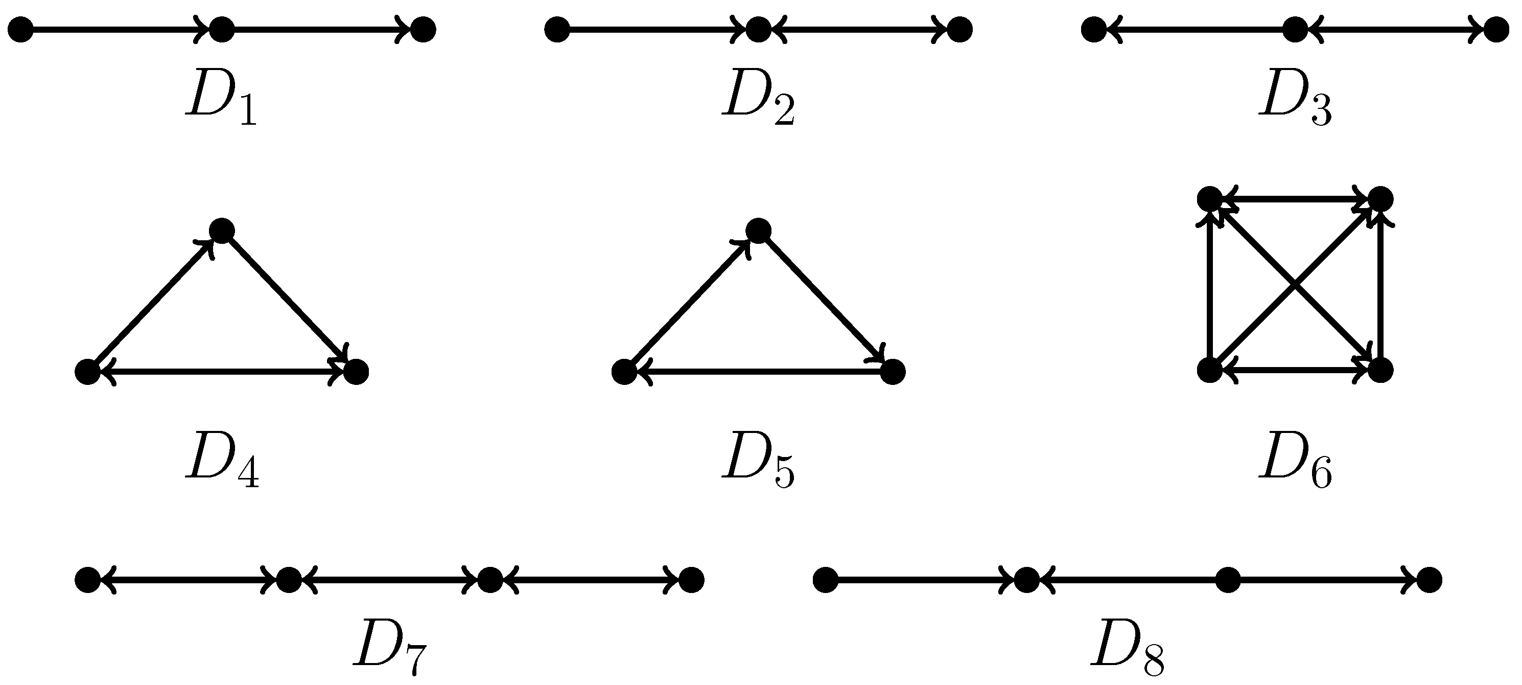
3. Preliminaries

For an integer i, $\left[i\right]$ denotes the set of all positive integers no greater than i.

A directed graph (digraph) is a tuple $G=(V,A)$, where V is the set of vertices of G and A is the set of arcs of G. An arc from a vertex v to another vertex $v^{\prime }$ is denoted by $(v,v^{\prime })$. For a digraph $G=(V,A)$, we define $E\left(G\right)=\left\{\right\{u,v\}:\{(u,v),(v,u)\}\cap A\ne \varnothing \}$ as the set of edges in the underlying undirected graph of G. For notational brevity, we denote an edge between two vertices v and u by $vu$. For a graph G (be it directed or undirected), we use $V\left(G\right)$ to denote the vertex set of G. Deleting an edge $vu$ from G means deleting all arcs between v and u. Thus, if we delete an edge $vu$ from G, we obtain a graph with vertex set V and arc set $A\setminus \left\{\right(v,u),(u,v\left)\right\}$. For $E^{\prime }\subseteq E\left(G\right)$, $G-E^{\prime }$ denotes the digraph obtained from G by deleting all edges in $E^{\prime }$. A graph G is considered to be F-$free$ if it does not contain an induced subgraph that is isomorphic to F. In this case, F is also referred to as the forbidden graph for G. In this paper, we use the branch vector $({\tau }_1,{\tau }_2,\dots ,{\tau }_r)$ to represent a branching rule that branches into r instances, where the maximum number of new parameters is $k-{\tau }_1$, $k-{\tau }_2$, …, $k-{\tau }_r$. The linear recurrence of the maximum number of leaves for this branch vector is $T\left(k\right)\le T(k-{\tau }_1)+T(k-{\tau }_2)+\dots +T(k-{\tau }_r)$. The DCGED problem is formally defined as follows:

 

Directed Co-Graph Edge Deletion (DCGED)

Input: A directed graph G and an integer k.

Question: $\exists E^{\prime }\subseteq E\left(G\right)$ so that $|E^{\prime }|\le k$ and $G-E^{\prime }$ is a directed co-graph?

4. Our Results

We first show the NP-hardness of DCGED, and we then present our algorithm for DCGED.

Theorem 1. 

DCGED is NP-hard.

Proof. 

Let $(G,k)$ be an instance of CGED. Recall that this problem determines whether we can remove, at most, k edges from G so that the resulting graph contains no paths of three edges as induced subgraphs. Let $G^{\prime }$ be the digraph obtained from G by changing each edge $uv$ with two arcs $(v,u)$ and $(u,v)$. Among all eight forbidden structures $D_1$–$D_8$, only in $D_7$ are all arcs bidirected; thus, it holds that there are, at most, k edges in G whose removal results in a co-graph, if and only if removing the corresponding k edges in $G^{\prime }$ results in a directed co-graph. Then, the theorem follows from the NP-hardness of CGED [6]. □

Our second main contribution is a single exponential time algorithm for the DCGED problem based on branching. For a collection $\{E_1,E_2,\dots ,E_j\}$ of subsets of edges, a branching rule that splits the instance into j subinstances, where the i-th subinstance, $i\in \left[j\right]$, is obtained from the original instance by deleting exactly the edges in $E_i$ and decreasing the parameter k by $|E_i|$, is denoted by $\{-E_1,-E_2,\dots ,-E_j\}$. Here, each $-E_i$ is called a branching case of the branching rule. For clarity, we use $\{-e:e\in E_i\}$ to denote the branching case $-E_i$; to describe a branching rule, we list all its branching cases, with one in each line.

Theorem 2. 

DCGED can be solved in time $O\left({2.733}^k\right)$.

Proof. 

Let $(G,k)$ be an instance of DCGED. We now discuss branching rules for the problem. We stress that the branching rules are iteratively applied to the instance in an order where, when a branching rule delineated below is applied, all rules introduced before are exhaustively applied.

Clearly, direct branching on the edges of an induced $D_i$, $i\in \left[3\right]$ has a branching factor of 2, and direct branching on the edges of an induced $D_i$, $i\in \{4,5\}$ has a branching factor of 3. However, after deleting any edge in an induced $D_4$ ($D_5$), at least one new induced $D_1$, $D_2$, or $D_3$ emerges. Therefore, at least two edges need to be deleted in the induced $D_4$ ($D_5$). Its branching vector is $(2,2,2)$, resulting in a branching rule with a branching factor of $\sqrt{3}$, which is less than $1.733$.

Now, we proceed to the branching rules for $D_6$. It can be observed that in order to destroy an induced $D_6$ and some induced $D_1$–$D_5$ occurring after the deletion of some edges in the $D_6$, we need to delete at least three edges. To facilitate our analysis, let the vertices of an induced $D_6$ be labeled as in Figure 2. The detailed branching cases are as follows.

(1)

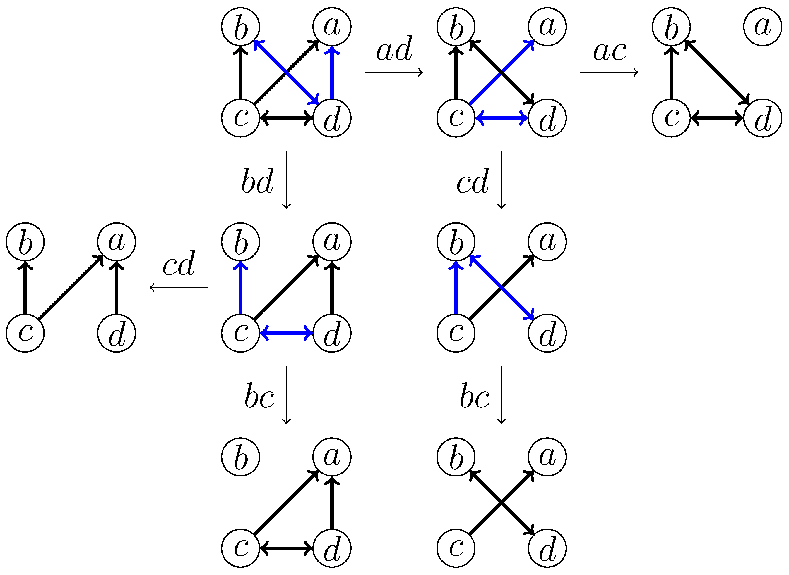
Deletion of the edge $ab$

After deleting $ab$, vertices a, d, and b form an induced $D_3$. The deletion of $ad$ or $bd$ will induce new forbidden structures, which will trigger the deletion of further edges. In particular, we have the following branching cases, as shown in Figure 3.

• $\{-ab,-ad,-ac\}$
• $\{-ab,-ad,-cd,-bc\}$
• $\{-ab,-bd,-cd\}$
• $\{-ab,-bd,-bc\}$

(2)

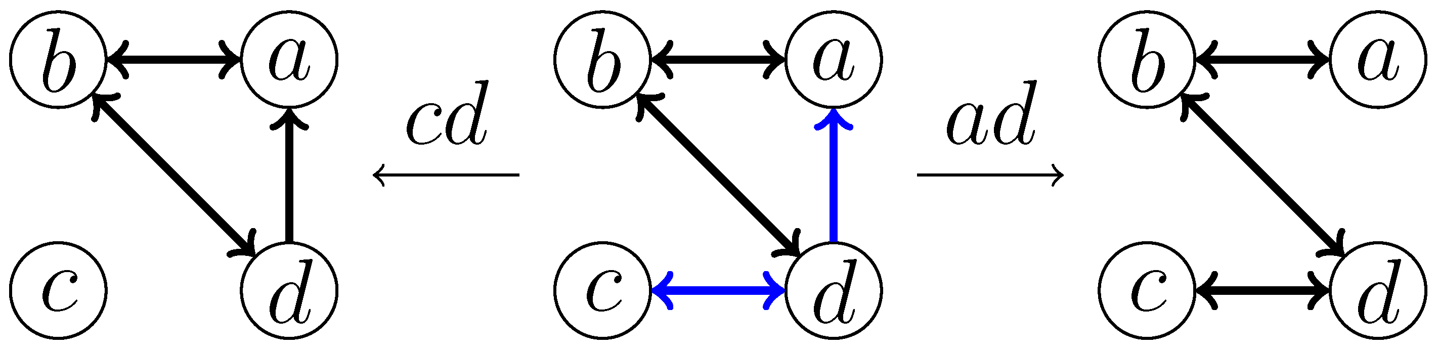
Deletion of the edge $ac$

After deleting $ac$, $\{a,b,c\}$ induces a $D_2$ and $\{a,c,d\}$ induces a $D_3$. The deletion of $ab$ is covered in Case (1). Thus, we need only to consider the deletion of edge $bc$ to destroy the $D_2$. It follows that the branching cases $\{-ac,-bc,-ad\}$ and $\{-ac,-bc,-cd\}$ cover all potential solutions where the edge $ac$ is deleted, as shown in Figure 4 (in the first branching case, we obtain an induced $D_7$, meaning that further edges need to be deleted. However, as this does not improve the worst-case branching factor, and the induced $D_7$s are handled by branching rules introduced later, to simplify the presentation, we do not discuss this improvement).

(3)

Deletion of the edge $ad$

After deleting $ad$, vertices a, c, and d form an induced $D_3$, and since the deletion of $ac$ is covered in Cases (1) and (2), we consider the deletion of $cd$. Observe now that b, c, and d form an induced $D_2$. If we delete $bc$, then a, b, and c form an induced $D_2$, implying that at least one of $ab$ and $ac$ needs to be deleted, which is covered in Cases (1) and (2). Therefore, we do not need to consider the case where $bc$ is deleted. In other words, in this case, we need only the branching case $\{-ad,-cd,-bd\}$.

(4)

Deletion of the edge $bc$

The deletion of $bc$ triggers the deletion of at least one of $ab$ and $ac$, both of which are covered by previous cases.

(5)

Deletion of the edge $bd$

After deleting $bd$, an induced $D_2$ formed by a, b, and d and an induced $D_3$ formed by b, c, and d occur. To destroy the $D_2$, at least one of $ab$ and $ad$ needs to be deleted, both of which are covered by previous cases.

(6)

Deletion of the edge $cd$

After deleting the edge $cd$, the vertices b, c, and d form an induced $D_2$, inviting the further deletion of at least one of $bc$ and $bd$, both of which are covered by previous cases.

To summarize, to destroy $D_6$, we apply the following branching rule, which has a branching vector of $(3,3,3,3,3,3,4)$ and a corresponding maximum branching factor of 1.870:

• $\{-ab,-ad,-ac\}$
• $\{-ab,-ad,-cd,-bc\}$
• $\{-ab,-bd,-cd\}$
• $\{-ab,-bd,-bc\}$
• $\{-ac,-bc,-ad\}$
• $\{-ac,-bc,-cd\}$
• $\{-ad,-cd,-bd\}$

Now, we consider the forbidden structures $D_7$ and $D_8$. We first apply branching rules satisfying the following condition: the deletion of some edges in an induced $D_7$ or $D_8$ results in a new induced $D_i$s, where $i\in \left[3\right]$. Specifically, we assume that there is an induced $D_7$ or $D_8$ denoted by H in G so that the deletion of some edge $xy$ from H results in an induced $D_i$, where $i\in \left[3\right]$, denoted by $H^{\prime }$. Let v denote the third vertex in $H^{\prime }$. It is clear that v is the middle vertex of $H^{\prime }$ (i.e., the one with degree two in the underlying graph of $H^{\prime }$). Let e and $e^{\prime }$ be the other two edges in H other than $xy$. Then, we exert the following branching rule that has a branching factor $1+\sqrt{3}<2.733$:

• $\{-e\}$
• $\{-e^{\prime }\}$
• $\{-xy,-vx\}$
• $\{-xy,-vy\}$

We continue our branching for $D_7$ as follows. Let H be an induced $D_7$. If H is a connected component, we directly delete it from G and decrease k by one. Assume now that there exists at least one vertex v not in H but adjacent to at least one vertex from H. By symmetry, and by the assumption that none of the above-discussed branching rules are applicable, we need to consider the following cases.

Case 

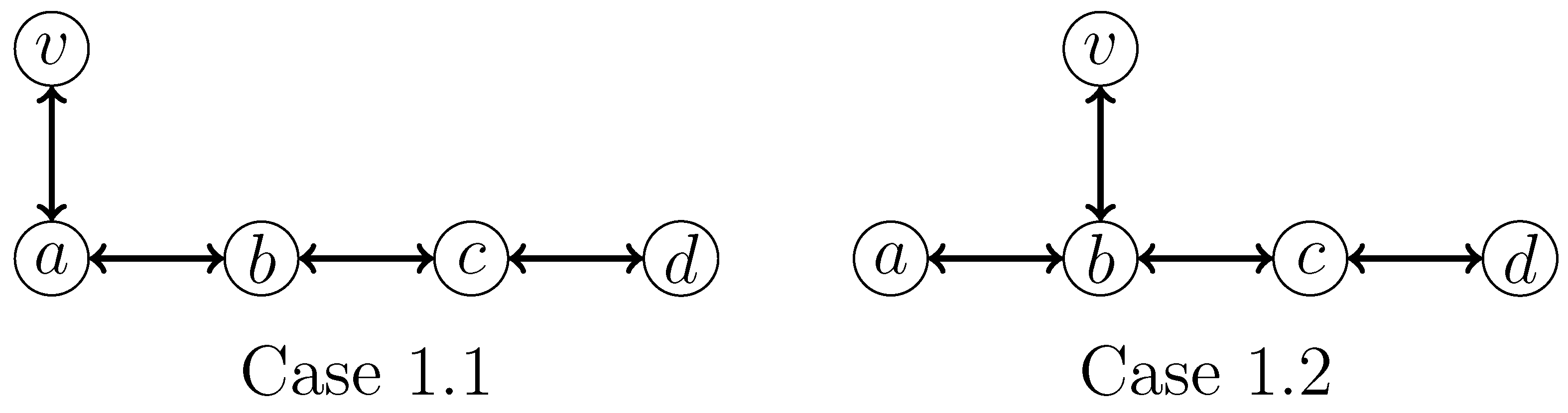
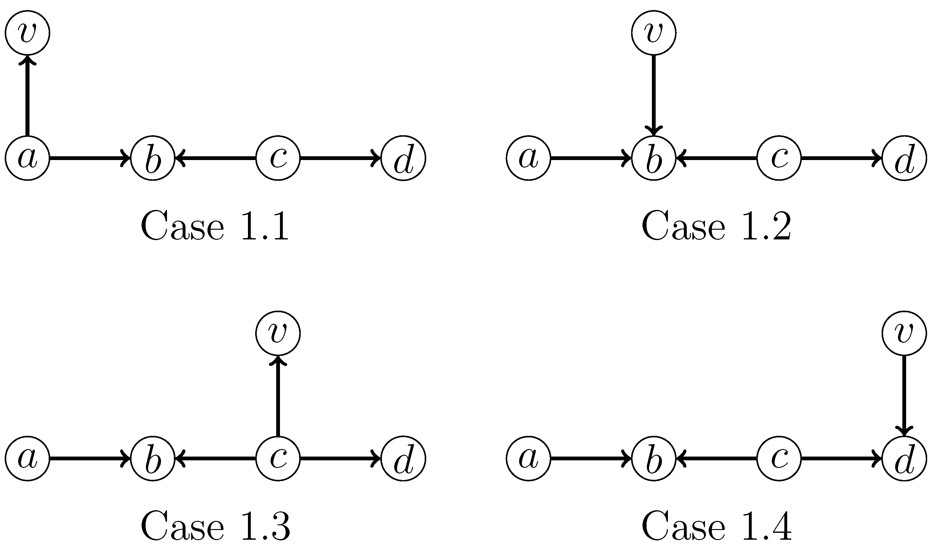
1: v has exactly one neighbor in H.

We have two subcases to consider, as shown in Figure 5.

In both subcases, there are indeed two induced $D_7$s; hence, deleting only one edge is insufficient. Specifically, for Case 1.1, we apply the following branching rule:

• $\{-ab\}$
• $\{-bc\}$
• $\{-av,-cd\}$

For Case 1.2, we apply the following branching rule:

• $\{-cd\}$
• $\{-bc\}$
• $\{-ab,-vb\}$

Both branching rules have the same branching vector of $(1,1,2)$ and a corresponding maximum branching factor of $1+\sqrt{2}<2.4143$.

Case 

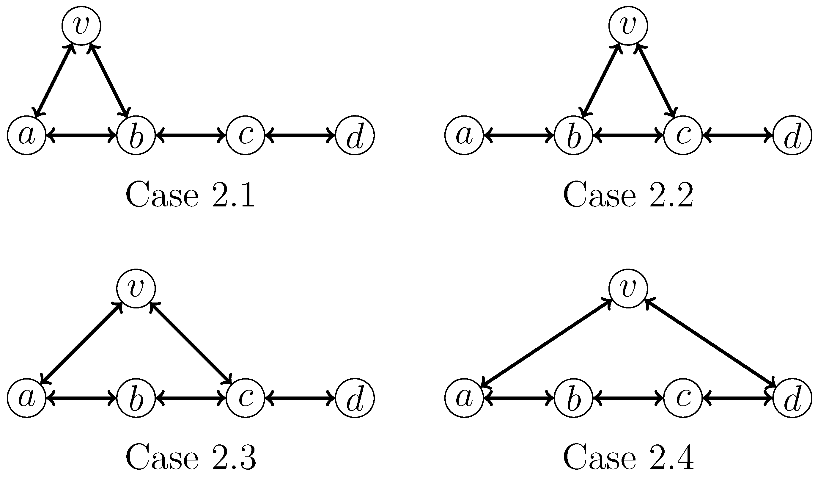
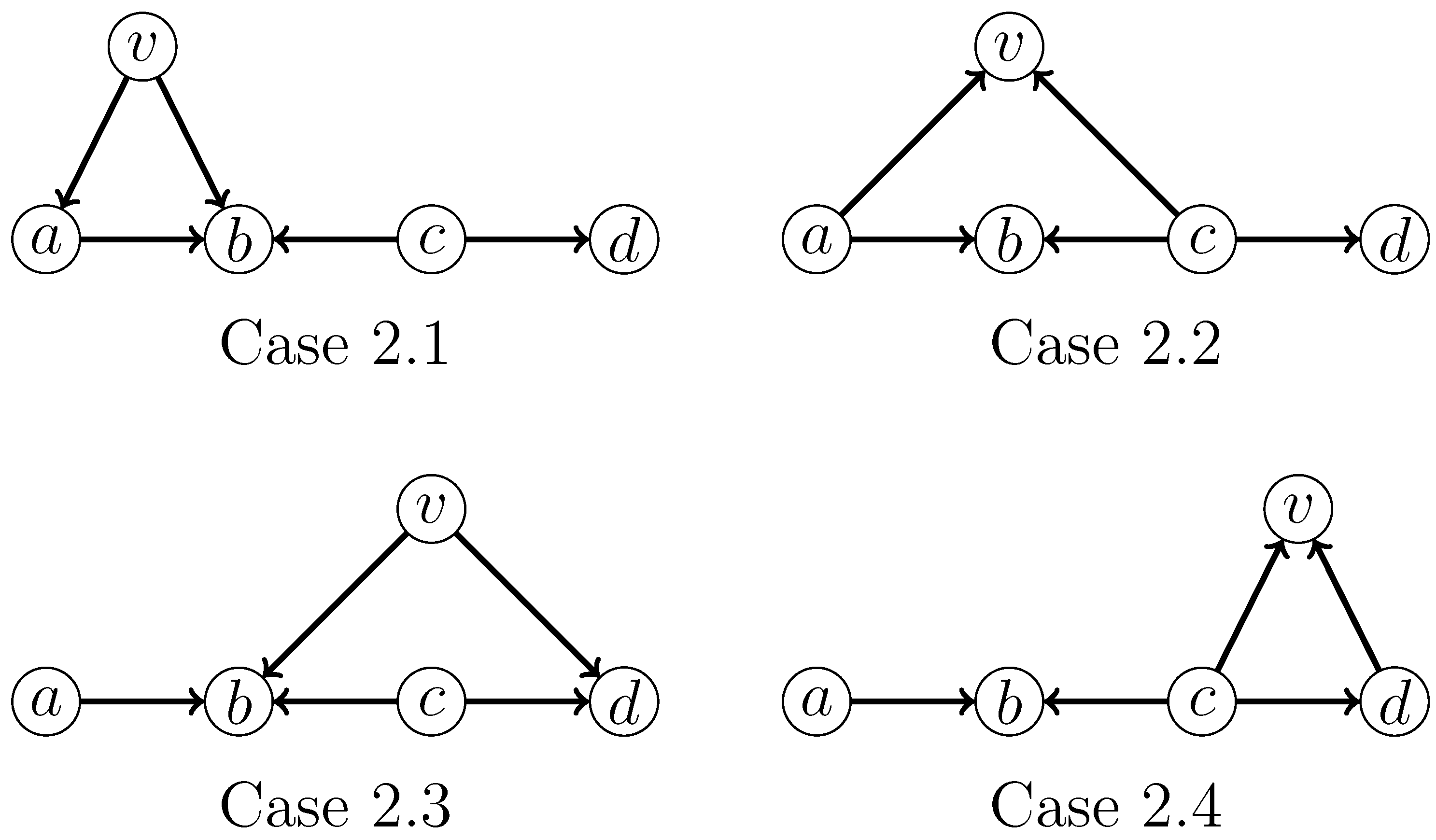
2: v has exactly two neighbors in H.

We need to consider the four subcases shown in Figure 6.

For Case 2.1, we apply the following branching rule, where the branching vector is $(1,1,2)$, corresponding to the branching factor $1+\sqrt{2}<2.4143$:

• $\{-cd\}$
• $\{-bc\}$
• $\{-ab,-vb\}$

For Case 2.2, we apply the following branching rule, where the branching vector is $(1,1,2,2)$, corresponding to the branching factor $1+\sqrt{3}<2.733$:

• $\{-ab\}$
• $\{-cd\}$
• $\{-bc,-vb\}$
• $\{-bc,-vc\}$

For Case 2.3, we apply the following branching rule, where the branching vector is $(1,2,2,2,2)$ and the branching factor is $\frac{1+\sqrt{17}}{2}<2.5616$:

• $\{-cd\}$
• $\{-va,-ab\}$
• $\{-va,-bc\}$
• $\{-vc,-ab\}$
• $\{-vc,-bc\}$

For Case 2.4, we apply the following branching rule, where the branching vector is $(1,1,2)$ and the branching factor is $1+\sqrt{2}<2.4143$:

• $\{-ab\}$
• $\{-bc\}$
• $\{-va,-cd\}$

Case 

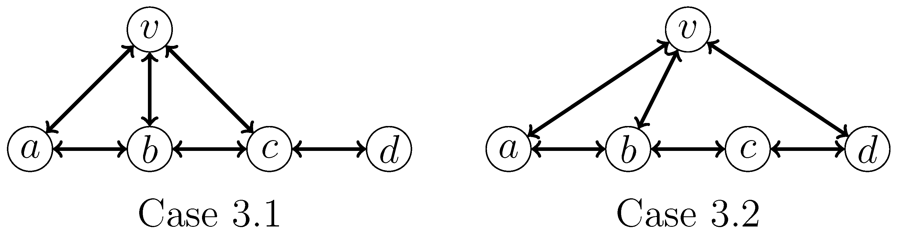
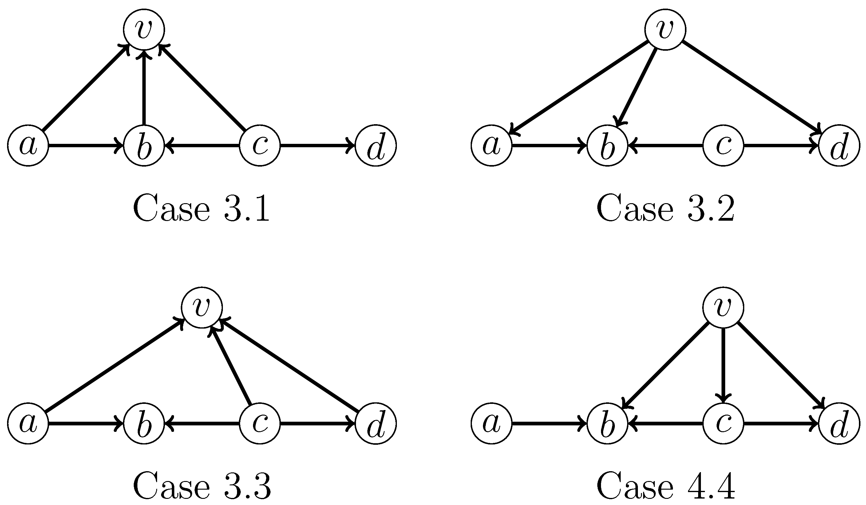
3: v has exactly three neighbors in H.

Figure 7 depicts all subcases that we need to consider. For Case 3.1, we apply the following branching rule, which has a branching vector of $(1,2,2,3,3)$ and a corresponding maximum branching factor of $2.2696$:

• $\{-cd\}$
• $\{-va,-ab\}$
• $\{-va,-bc,-vb\}$
• $\{-vc,-bc\}$
• $\{-vc,-ab,-vb\}$

For Case 3.2, we apply the following branching rule, which has a branching vector of $(2,2,2,2,3,3,3,3)$ and a corresponding maximum branching factor of $2.3830$:

• $\{-cd,-bc\}$
• $\{-cd,-vb,-va\}$
• $\{-cd,-vb,-ab\}$
• $\{-cd,-vd\}$
• $\{-bc,-vb,-va\}$
• $\{-bc,-vd\}$
• $\{-ab,-va\}$
• $\{-ab,-vd,-vb\}$

Case 

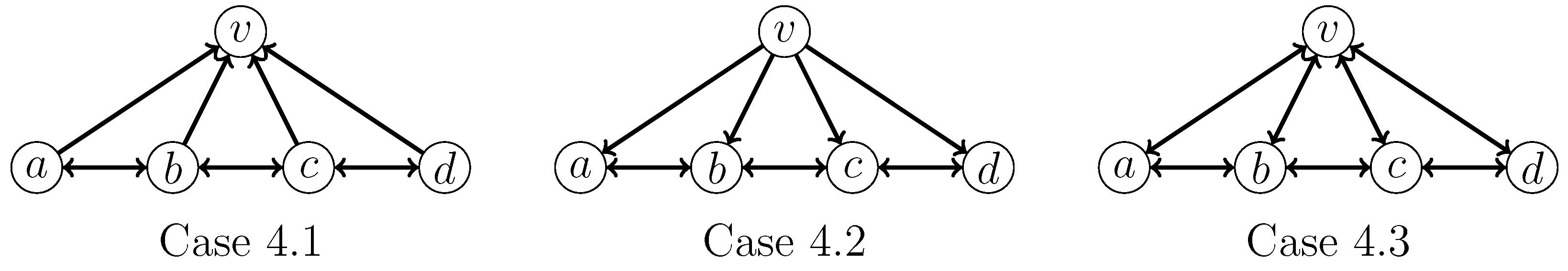
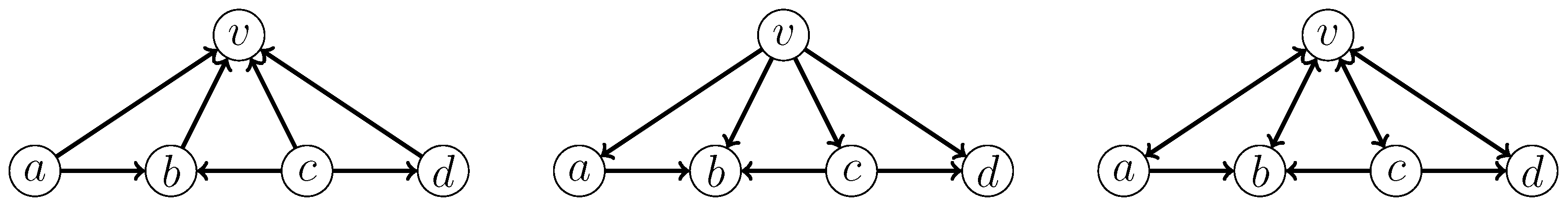
4: v is adjacent to all vertices of H.

When none of the branching rules introduced above are applicable, if a vertex is adjacent to one vertex of H, then it is adjacent to all vertices of H, and, moreover, the subgraph induced by this vertex and all vertices of H is isomorphic to one of the graphs in Figure 8. Then, by the symmetry between the edges $ab$ and $cd$, the branching cases $\{-ab\}$ and $\{-bc\}$ of branching factor 2 are sufficient in this case.

Finally, we discuss branching rules for $D_8$. Let H be an induced $D_8$. If H is a connected component of G, we directly delete H from G and decrease k by one. Otherwise, let v be a vertex not in H but adjacent to some vertices of H. Assuming that none of the branching rules introduced above are applicable, we need to consider the following cases.

Case 

1: v is adjacent to exactly one vertex of H.

All subcases that need to be considered are shown in Figure 9.

For Case 1.1, we apply the branching rule:

• $\{-ab\}$
• $\{-bc\}$
• $\{-va,-cd\}$

For Case 1.2, we apply the branching rule:

• $\{-cd\}$
• $\{-bc\}$
• $\{-vb,-ab\}$

For Case 1.3, we apply the branching rule:

• $\{-ab\}$
• $\{-bc\}$
• $\{-vc,-cd\}$

For Case 1.4, we apply the branching rule:

• $\{-cd\}$
• $\{-bc\}$
• $\{-vd,-ab\}$

The above four branching rules have the same branching vector of $(1,1,2)$ and a corresponding maximum branching factor of $1+\sqrt{2}<2.4143$.

Case 

2: v has exactly two neighbors from H.

All subcases that need to be considered are shown in Figure 10.

For Case 2.1, we apply the following branching rule, where the branching vector is $(1,1,2)$ and the corresponding branching factor is $1+\sqrt{2}<2.4143$:

• $\{-bc\}$
• $\{-cd\}$
• $\{-vb,-ab\}$

For Case 2.2, we apply the following branching rule, where the branching vector is $(1,2,2,2,2)$ and the corresponding branching factor is $\frac{1+\sqrt{17}}{2}<2.5616$:

• $\{-cd\}$
• $\{-va,-ab\}$
• $\{-va,-bc\}$
• $\{-vc,-ab\}$
• $\{-vc,-bc\}$

For Case 2.3, we apply the following branching rule, where the branching vector is $(1,2,2,2,2)$ and the corresponding branching factor is $\frac{1+\sqrt{17}}{2}<2.5616$:

• $\{-ab\}$
• $\{-vb,-bc\}$
• $\{-vb,-cd\}$
• $\{-vd,-bc\}$
• $\{-vd,-cd\}$

For Case 2.4, we apply the following branching rule, where the branching vector is $(1,1,2)$ and the corresponding branching factor is $1+\sqrt{2}<2.4143$:

• $\{-ab\}$
• $\{-bc\}$
• $\{-vc,-cd\}$

Case 

3: v has exactly three neighbors from H.

All subcases that need to be considered are shown in Figure 11.

For Case 3.1, we apply the following branching rule, which has a branching vector of $(1,2,2,3,3)$ and a corresponding maximum branching factor of $2.2696$:

• $\{-cd\}$
• $\{-va,-ab\}$
• $\{-va,-bc,-vb\}$
• $\{-vc,-bc\}$
• $\{-vc,-ab,-vb\}$

For Case 3.2, we apply the following branching rule, which has a branching vector of $(2,2,2,2,3,3,3,3)$ and a corresponding maximum branching factor of $2.3830$:

• $\{-bc,-vd\}$
• $\{-bc,-vb,-va\}$
• $\{-cd,-vd\}$
• $\{-cd,-vb,-va\}$
• $\{-cd,-bc\}$
• $\{-ab,-va\}$
• $\{-ab,-vb,-vd\}$
• $\{-ab,-vb,-cd\}$

For Case 3.3, we apply the following branching rule, which has a branching vector of $(2,2,2,2,3,3,3,3)$ and a corresponding maximum branching factor of $2.3830$:

• $\{-cd,-vc,-av\}$
• $\{-cd,-vc,-ab\}$
• $\{-cd,-vd\}$
• $\{-vc,-bc,-vd\}$
• $\{-va,-bc\}$
• $\{-ab,-bc\}$
• $\{-ab,-va\}$
• $\{-vc,-ab,-vd\}$

For Case 3.4, we apply the following branching rule, which has a branching vector of $(1,2,2,3,3)$ and a corresponding maximum branching factor of $2.2696$:

• $\{-ab\}$
• $\{-vb,-bc\}$
• $\{-vb,-cd,-vc\}$
• $\{-vd,-bc,-vc\}$
• $\{-vd,-cd\}$

Case 

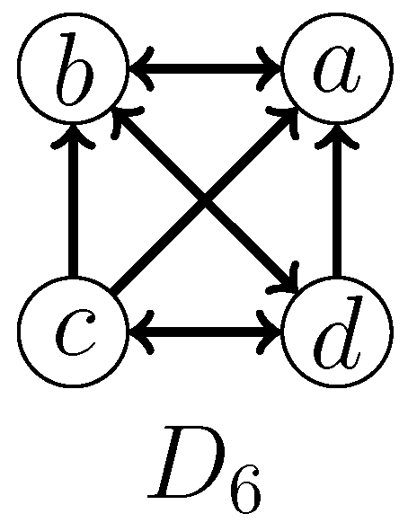
4: v is adjacent to all vertices of H.

Let us consider a graph where none of the branching rules introduced so far are applicable, which is called a reduced graph. It is easy to verify that in a reduced graph, for any induced $D_8$ and any vertex v adjacent to all vertices of $D_8$, the subgraph induced by the vertex v and the $D_8$ is isomorphic to one of the graphs in Figure 12. Two important observations are formulated below.

Observation 1. Let G be a reduced graph. Then, all induced $D_8$s in G are pairwise vertex disjoint.

Observation 2. Let G be a reduced graph. Then, deleting any edge from an induced $D_8$ in G does not yield any new induced forbidden structures ($D_1$–$D_8$).

Let i be the number of all induced $D_8$ in a reduced graph G. By Observation 1, we need to delete i edges to destroy all the induced $D_8$s in G. By Observation 2, the resulting graph is a directed co-graph. In light of this fact, when we arrive at a reduced graph at a branching node, we determine that the given instance is a YES-instance if there are, at most, k induced $D_8$s in the reduced graph.

Throughout the algorithm, when we reach a branching node whose associated parameter k is zero, we immediately conclude that the given instance is a YES-instance if the graph associated with the branching node is a directed co-graph. Then, as the worst branching factor is $2.733$, the branch-and-bound algorithm runs in time $O(2.{733}^k)$. □

5. Conclusions

We showed that DCGED is NP-hard and developed a branching algorithm for DCGED with a running time of $O\left({2.733}^k\right)$, which significantly improves upon the brute-force algorithm’s running time of $O\left(6^k\right)$.

An obvious direction for future research is to further improve our algorithm. As mentioned earlier, when we consider the structural relationship between the forbidden subgraph and a neighboring vertex, we can effectively reduce the size of the search tree and obtain more effective branch rules. Therefore, it will be interesting to investigate whether it is possible to further reduce the size of the search tree and improve the efficiency of branch algorithms by considering deeper structural relationships between forbidden subgraphs and their neighboring vertices. Additionally, it would be interesting to examine whether the problem admits any polynomial kernels. Furthermore, we studied the case in which destroying the connection between two adjacent vertices incurs one unit cost, regardless of whether there are one or two arcs between them. It would be intriguing to investigate the variant in which removing any arc incurs one unit cost. Lastly, we utilized symmetry properties to further improve the size of the search tree for the DCGED problem, resulting in a more efficient branch algorithm. We believe that this property can be applied to more edge-modification problems.

References

- Crespelle, C.; Drange, P.G.; Fomin, F.V.; Golovach, P.A. A Survey of Parameterized Algorithms and the Complexity of Edge modification. Comput. Sci. Rev. 2023, 48, 100556. [Google Scholar] [CrossRef]
- Li, W.; Tang, X.; Yang, Y. An Improved Branching Algorithm for the Proper Interval Edge Deletion Problem. Front. Comput. Sci. 2022, 16, 162401. [Google Scholar] [CrossRef]
- Liu, Y.; Wang, J.; You, J.; Chen, J.; Cao, Y. Edge Deletion Problems: Branching Facilitated by Modular Decomposition. Theor. Comput. Sci. 2015, 573, 63–70. [Google Scholar] [CrossRef]
- Béchet, D.; de Groote, P.; Retoré, C. A Complete Axiomatisation for the Inclusion of Series-Parallel Partial Orders. In Proceedings of the Rewriting Techniques and Applications, 8th International Conference, RTA-97, Sitges, Spain, 2–5 June 1997; Lecture Notes in Computer Science. Comon, H., Ed.; Springer: Berlin/Heidelberg, Germany, 1997; Volume 1232, pp. 230–240. [Google Scholar] [CrossRef]
- Crespelle, C.; Paul, C. Fully Dynamic Recognition Algorithm and Certificate for Directed Cographs. Discret. Appl. Math. 2006, 154, 1722–1741. [Google Scholar] [CrossRef]
- El-Mallah, E.; Colbourn, C.J. The Complexity of Some Edge Deletion Problems. IEEE Trans. Circuits Syst. 1988, 35, 354–362. [Google Scholar] [CrossRef]
- Nastos, J.; Gao, Y. Bounded Search Tree Algorithms for Parametrized Cograph Deletion: Efficient Branching Rules by Exploiting Structures of Special Graph Classes. Discret. Math. Algorithms Appl. 2012, 4, 1250008. [Google Scholar] [CrossRef]
- Guillemot, S.; Havet, F.; Paul, C.; Perez, A. On the (Non-)Existence of Polynomial Kernels for Pl-Free Edge Modification Problems. Algorithmica 2013, 65, 900–926. [Google Scholar] [CrossRef]
- Bretscher, A.; Corneil, D.G.; Habib, M.; Paul, C. A Simple Linear Time LexBFS Cograph Recognition Algorithm. SIAM J. Discret. Math. 2008, 22, 1277–1296. [Google Scholar] [CrossRef]
- Schmitz, Y.; Wanke, E. The Directed Metric Dimension of Directed Co-Graphs. arXiv 2023, arXiv:2306.08594. [Google Scholar]
- Gurski, F.; Komander, D.; Rehs, C. How to Compute Digraph Width Measures on Directed Co-Graphs. Theor. Comput. Sci. 2021, 855, 161–185. [Google Scholar] [CrossRef]
- Gurski, F. Dynamic Programming Algorithms on Directed Cographs. Stat. Optim. Inf. Comput. 2017, 5, 35–44. [Google Scholar] [CrossRef][Green Version]
Disclaimer/Publisher’s Note: The statements, opinions and data contained in all publications are solely those of the individual author(s) and contributor(s) and not of MDPI and/or the editor(s). MDPI and/or the editor(s) disclaim responsibility for any injury to people or property resulting from any ideas, methods, instructions or products referred to in the content. |
© 2024 by the authors. Licensee MDPI, Basel, Switzerland. This article is an open access article distributed under the terms and conditions of the Creative Commons Attribution (CC BY) license (https://creativecommons.org/licenses/by/4.0/).
Share and Cite
Li, W.; Yang, X.; Xu, C.; Yang, Y. An FPT Algorithm for Directed Co-Graph Edge Deletion. Algorithms 2024, 17, 69. https://doi.org/10.3390/a17020069
Li W, Yang X, Xu C, Yang Y. An FPT Algorithm for Directed Co-Graph Edge Deletion. Algorithms. 2024; 17(2):69. https://doi.org/10.3390/a17020069
Chicago/Turabian StyleLi, Wenjun, Xueying Yang, Chao Xu, and Yongjie Yang. 2024. "An FPT Algorithm for Directed Co-Graph Edge Deletion" Algorithms 17, no. 2: 69. https://doi.org/10.3390/a17020069
APA StyleLi, W., Yang, X., Xu, C., & Yang, Y. (2024). An FPT Algorithm for Directed Co-Graph Edge Deletion. Algorithms, 17(2), 69. https://doi.org/10.3390/a17020069