1. Introduction
The unrelated parallel machine scheduling problem is an important combinatorial optimisation problem with frequent applications in the real world [
1], such as task scheduling [
2], device scheduling [
3], and manufacturing [
4]. Since the problem is NP-hard, it is traditionally solved using various metaheuristic optimisation methods [
5,
6]. However, since real-world problems are often dynamic in nature, traditional optimisation approaches that continuously improve potential solutions are usually not directly applicable. The reason for this is that not all information about the problem under consideration may be known, and in this case, it is not possible to construct a complete solution. This was the motivation for researching alternative methods that can be used to solve dynamic problems such as dispatching rules.
Dispatching rules (DRs) have emerged as an alternative solution method for solving various scheduling problems, mostly dynamic problem variants [
7]. They represent simple constructive heuristics that solve the problem incrementally by making decisions about which job to schedule next based solely on the information currently available in the system. Therefore, such rules can react quickly to the changing problem environment, as they construct the solution based only on the currently available information. As new information becomes available, they can take it into account when constructing the solution. Although many DRs have been proposed over the years [
7], they have been developed for a limited number of problem variants and scheduling criteria. In addition, the developed DRs perform scheduling decisions using simple heuristic strategies, which affects the quality of the plans they produce.
To address the above problems, various methods based on evolutionary computation and machine learning have been used over the years to automatically design new DRs for various problems [
8,
9,
10]. One of the most commonly used methods for this purpose is genetic programming [
11]. GP is an evolutionary computational method developed to enable the generation of various mathematical expressions and even computer programmes [
12]. It has been applied in many fields, where it has achieved competitive results with humans [
13], proving its effectiveness. In recent years, however, GP has established itself as the leading hyperheuristic method [
14,
15], a method used to automatically develop new heuristics.
In the context of DRs, GP is used to generate an expression, often referred to as a priority function, that is used by the DR to rank all decisions at each decision point and select the appropriate decision [
16]. GP generates the expression based on a set of defined problem characteristics, which it attempts to combine in a meaningful way to determine the optimal scheduling decision at each decision point. Therefore, it is necessary to provide GP with all the relevant information about the problem in the form of terminal nodes representing certain features of the problem. However, an incomplete or wrong choice of terminal nodes can result in myopic DRs that offer poor performance [
17]. Regardless, this step is often overlooked, and quite often only the most basic problem information is used as terminal nodes without a selection of appropriate nodes. Naturally, providing too many terminal nodes again has the drawback that the search space of the method grows exponentially, making it more difficult to find high-quality solutions. Although the definition and choice of appropriate terminal nodes is an important decision that significantly affects the quality and complexity of DRs, it has not yet been investigated in the context of the automated design of DRs for unrelated machine environments. Thus, there is no guarantee that the terminal nodes currently applied in the literature are really the most appropriate or whether the results could be improved by applying a different set of terminal nodes.
The aim of this study is to perform a detailed investigation of the influence of different problem properties on the quality of DRs automatically developed by GP for unrelated machine scheduling problems. The motivation for this is to determine the set of the most suitable terminal nodes, with which GP can generate DRs that perform well across a wide range of problem instances. This is done in a sequential manner, where first, simple atomic features are analysed, representing only the most basic information about the problem. Then, composite features are added to the set of terminals to investigate whether by including more sophisticated terminal nodes, either designed automatically or manually, they can improve the performance of the generated DRs. Naturally, only providing the terminal nodes is not enough, since a too-large terminal set can negatively affect the results simply due to a too-large solution space that the algorithm needs to traverse. Therefore, to select the appropriate feature set, we use the backward sequential feature selection method, which is commonly used in the literature for this purpose, but also investigate the ability of GP to perform feature selection by using the frequency of occurrence of nodes in the expressions as a criterion for selecting the appropriate features. From the obtained results, we investigate how the different node sets that were obtained influence not only the performance and complexity of the generated DRs but also the performance of different methods in selecting the appropriate features.
The contributions of this study can be summarised as follows:
Analysis of how different types of terminal nodes influence the effectiveness of GP to generate good quality DRs and their complexity.
Construction of new terminal nodes based on the frequency of occurrence of sub-expressions in the generated DRs.
Application and comparison of two feature selection methods to determine appropriate terminal node sets.
The rest of this study is organised as follows.
Section 2 outlines the relevant literature on the generation of DRs with GP. The necessary background information about the problem under consideration and the application of GP to generate DRs is given in
Section 3. The methodology used to conduct the investigation in this paper is described in
Section 4.
Section 5 describes the design of the experimental study and discusses the results obtained. A more in-depth analysis of the results obtained is presented in
Section 6. Finally,
Section 7 concludes this paper and provides guidance for future research.
2. Literature Review
The automated generation of DRs has its roots in the pioneering studies of Miyashita [
18] and Dimopoulos and Zalzala [
19]. These studies showed that GP can be efficiently used to design new DRs for various scheduling problems. Since then, GP has been applied in numerous studies to generate DRs for various problems, such as the parallel machine scheduling problem [
20], flexible job shop problem [
21], resource-constrained project scheduling problem [
22], and one-machine variable capacity problem [
23].
Over the years, many research directions have been explored in the context of the automated design of DRs. One line of research has focused on investigating different representations for DRs. In [
24], the authors compared three DR representations: one that generates an expression that selects an existing DR based on system properties to make the scheduling decision, one that generates a new DR from basic system information, and one that combines the previous two approaches. The results showed that the first approach was inferior to the other two approaches. In [
25], the potential of GP to generate DRs was compared with that of artificial neural networks. The results showed that both methods performed similarly, but GP developed interpretable and more user-friendly DRs. In [
26], the authors investigated several evolutionary algorithms for developing DRs and found that their performance was similar in most cases, although some resulted in simpler DRs. Another line of research focused on the generation of DRs for multi-objective scheduling problems, which were considered in [
27,
28,
29] for the job shop problem and [
30] for the unrelated machine scheduling problem.
Ensemble learning is one of the most widely considered topics related to DR creation, as it has the potential to significantly improve the performance of individual DRs. This topic has been studied from many aspects, including methods used to construct ensembles [
31,
32,
33], methods used to aggregate the decisions of individual DRs in the ensemble [
34,
35], and the application of ensemble learning for multi-objective problems [
36]. Another way to improve the performance of automatically generated DRs is the application of surrogate models [
37,
38] and local search [
39], both of which have been shown to improve the performance of GP. Another recent research trend is the application of multitask learning in GP, which enables knowledge transfer between individuals to solve different types of problems [
40].
Only limited attention has been given to the issues of feature selection and construction in the context of automatic generation of DRs, and this has focused mainly on the job shop scheduling problem. In [
41], the authors proposed a feature selection algorithm that is embedded in GP and based on niching. This feature selection method takes into account both the fitness of the individuals in which the features occur and the frequency of occurrence of these features. The experimental results showed that the proposed approach can select features that lead to better results compared to using the entire feature set. In [
42], the authors considered feature selection in the context of developing DRs for the flexible job shop problem. In this approach, two terminal sets are used and, therefore, features need to be selected for each of them simultaneously. A GP approach with adaptive search based on the frequency of features was proposed in [
43] and was shown to perform better compared to standard GP in some scenarios. Another feature selection approach was proposed in [
44], which led to simpler DRs that achieved comparable performance to those developed without feature selection. Finally, in [
45], the authors considered feature construction in addition to feature selection, but no follow-ups or extensions to this original research were conducted. Overviews of the literature on the remaining studies dealing with the automated design of DRs for various scheduling problems can be found in [
8,
9,
10].
The importance of selecting suitable problem features when using GP to create DRs was discussed in [
17]. However, studies in this field rarely explore the definition of the features used in solving a particular problem. On the contrary, a particular set of features is usually defined based on previous user experiences, without further investigation into whether this terminal set is really the most appropriate. As can be seen from the previous literature review, although several studies deal with feature selection, they focus on the algorithmic aspect rather than on which features should be used or how they should be designed. Therefore, this study provides a deeper investigation into the definition and selection of features in the automated development of DRs for unrelated machine environments.
3. Background
As mentioned previously, the unrelated machine environment appears in many real-world scenarios, such as the manufacturing of pipes, manufacturing cells, distributing jobs in heterogeneous systems, and scheduling in the textile industry, among others [
6]. Many of those problems are dynamic in nature, meaning that certain aspects of the problem are not known at the beginning of the system’s execution. In such cases, DRs represent the method of choice for solving such problems [
7]. However, the performance of existing DRs is quite limited, and they are usually designed for very specific problem variants, thus limiting their performance and generalisation ability. This means that it is required to design DRs for all the different problem variants that are considered. Since it is difficult to manually design DRs for all the available problem variants, the concept of the automated design of DRs has garnered significant attention. One of the most prominent and commonly used approaches for this purpose is GP, which has been successfully used to generate new DRs for various problems.
3.1. Unrelated Parallel Machine Scheduling Problem
In the unrelated machine scheduling problem, a set of jobs must be scheduled and executed on a scarce set of machines [
46]. Each job contains certain properties that are taken into account in scheduling decisions, such as:
—the processing time of job j on machine i.
—the release time of job j, which specifies the earliest time at which the job can be considered for scheduling.
—the due date of job j, which specifies the time by which the job should finish with its execution.
—the weight of job j, which indicates the importance of the job.
Each machine can only process one job at a time. As soon as a machine starts executing a job, it must complete it before it can start executing another job.
Many criteria can be considered and optimised for this problem. In this study, we focus on minimising the total weighted tardiness criterion (
), defined as
, which is one of the most frequently optimised criteria in the literature, especially when considering dynamic environments [
6].
represents the tardiness of job
j and is defined as
, where
indicates the time at which job
j was completed. The tardiness, therefore, represents the time the job has been completed after its due date, whereas the total weighted tardiness is simply the combination of all tardiness values multiplied by the corresponding weights. By minimising
, we effectively minimise the times jobs are completed after their due date.
Using the standard notation
for scheduling problems [
47], the problem considered in this study can be specified as
. In this notation,
represents the machine environment, which in this case, is the unrelated machine environment (denoted by
R);
represents the additional constraints, which in this case, include the release times of the jobs (denoted by
); and
represents the optimised criterion, which in this case, is the total weighted tardiness (denoted by
). Moreover, the problem is considered under dynamic conditions, which means that not all information about the problem is available during the execution of the system. More precisely, no information about the jobs, including their arrival time, is known before they are released into the system. However, once they are released into the system, all their properties are known precisely, and the jobs can then be taken into account for scheduling.
The most suitable method for solving such dynamic problems is DRs [
7]. DRs consist of two parts: a schedule generation scheme (SGS) and a priority function (PF) [
48]. The SGS represents the algorithmic framework of the DR, which determines when and under what conditions it performs scheduling decisions. It also ensures that it only creates feasible schedules, for example, by checking that no machine executes two jobs at the same time. Algorithm 1 provides the definition of the SGS that is used by the automatically designed DRs. This SGS performs a scheduling decision every time at least one machine is available and there are unscheduled jobs in the system. It also ensures that no job is scheduled on a machine on which a job is already in progress.
| Algorithm 1 SGS used by generated DRs |
- 1:
while true do - 2:
Wait until at least one job and one machine are available - 3:
for all available jobs j and each machine i in m do - 4:
Calculate the priority of scheduling j on machine i - 5:
end for - 6:
for all available jobs do - 7:
Determine the machine with the best value - 8:
end for - 9:
while jobs whose best available machine exists do - 10:
Determine the best priority of all such jobs - 11:
Schedule the job with the best priority - 12:
end while - 13:
end while
|
One of the most important parts of the SGS is determining which scheduling decision to make at each decision time, i.e., which job should be scheduled on which machine. The SGS uses a PF to evaluate all available decisions. The best decision, determined by the lowest or highest rank, is then selected and executed. Over the years, PFs of varying complexity have been proposed in the literature [
7]. For example, the earliest due date (EDD) rule uses a PF defined as
, which means that jobs are executed in order according to their due dates. The EDD selects the jobs with the earliest due dates first, where jobs that need to be completed as quickly as possible take priority. The PF can, of course, be much more complex than that defined by the EDD. In fact, the PF is the most important part of any DR, and, therefore, great care needs to be taken when developing new and efficient PFs. However, manually designing meaningful PFs has proven to be quite a difficult and tedious task, which is why only a limited number of existing PFs are available [
7,
8].
3.2. Genetic Programming and Generating DRs
GP is a metaheuristic method based on the concept of natural evolution [
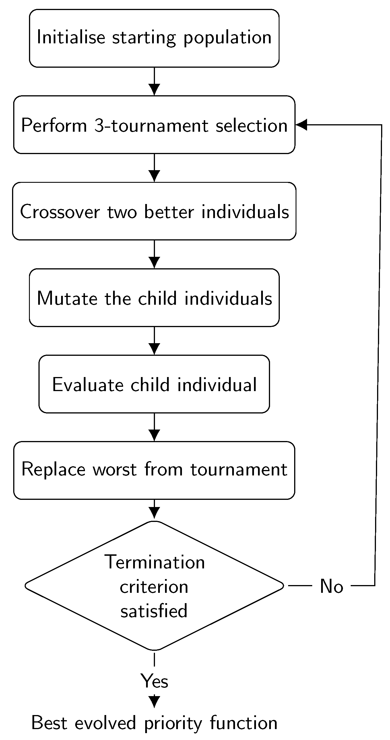
12]. It starts with a set, called the population, of randomly generated solutions, usually referred to as individuals. These individuals are evaluated using the fitness function, which calculates the fitness of each individual, i.e., a numerical measure of how well the individual solves a particular problem by optimising a certain criterion. GP then iteratively applies a series of genetic operators to these individuals in search of better solutions until a certain termination criterion is met. The operators that GP applies are selection, crossover, and mutation. With the selection operator, GP selects better individuals for the crossover operator and worse individuals to be eliminated from the population. The selected individuals are then used by the crossover operator, which combines their properties and creates a new individual that is potentially better than the individuals from which it was created. In addition, the newly created individual can be mutated with a certain probability to introduce random changes. The purpose of the mutation operator is to help the algorithm bypass local optima and restore lost genetic material in the population. This newly created individual then replaces one of the underperforming individuals in the population. With such a strategy, GP iteratively attempts to obtain better solutions through crossover and mutation and place them into the population, eliminating poor-quality individuals. The variant of the selection algorithm used in this study is described in Algorithm 2 [
48], and the flow diagram of the algorithm is shown in
Figure 1.
| Algorithm 2 The GP algorithm |
- 1:
Randomly create the population P and evaluate all individuals in it - 2:
while termination criterion is not met do - 3:
Randomly select 3 individuals from the population that form a tournament - 4:
Select the two better individuals - 5:
Crossover the selected individuals and create a new individual - 6:
Mutate the newly created individual with a certain probability - 7:
Evaluate the newly created individual - 8:
Replace the worst individual from the tournament with the newly created individual - 9:
end while
|
As already mentioned, solutions in GP are coded as expression trees consisting of function and terminal nodes. The function nodes are the inner nodes in the tree and represent various mathematical, logical, or other types of operations. The terminal nodes, on the other hand, appear as leaf nodes in the tree and represent different features of the problem. Therefore, the definition of terminal nodes is one of the most important decisions that must be made when applying GP to any problem. Through the evolutionary process, GP searches for the most appropriate expression to solve a given problem.
GP has been successfully used as a hyperheuristic method [
14,
49] to automatically generate heuristics for various types of combinatorial optimisation problems, such as scheduling problems [
50,
51], the travelling salesman problem [
52,
53], vehicle and arc routing problems [
54,
55,
56], the container relocation problem [
57], and the cutting stock problem [
15,
58]. When used to generate DRs for scheduling problems, GP has the task of finding a suitable PF that can be used by the DR to evaluate scheduling decisions. Each individual represents a potential PF, which is then used by the SGS, as defined in Algorithm 1, to evaluate its effectiveness for a given set of problem instances. To be able to meaningfully rank the various decisions in the scheduling problem, e.g., which job to schedule next, GP must have access to all relevant features of the problem via its terminal nodes. Therefore, the set of terminal nodes must contain relevant problem characteristics, such as the processing times of jobs, their due dates, weights, and so on.
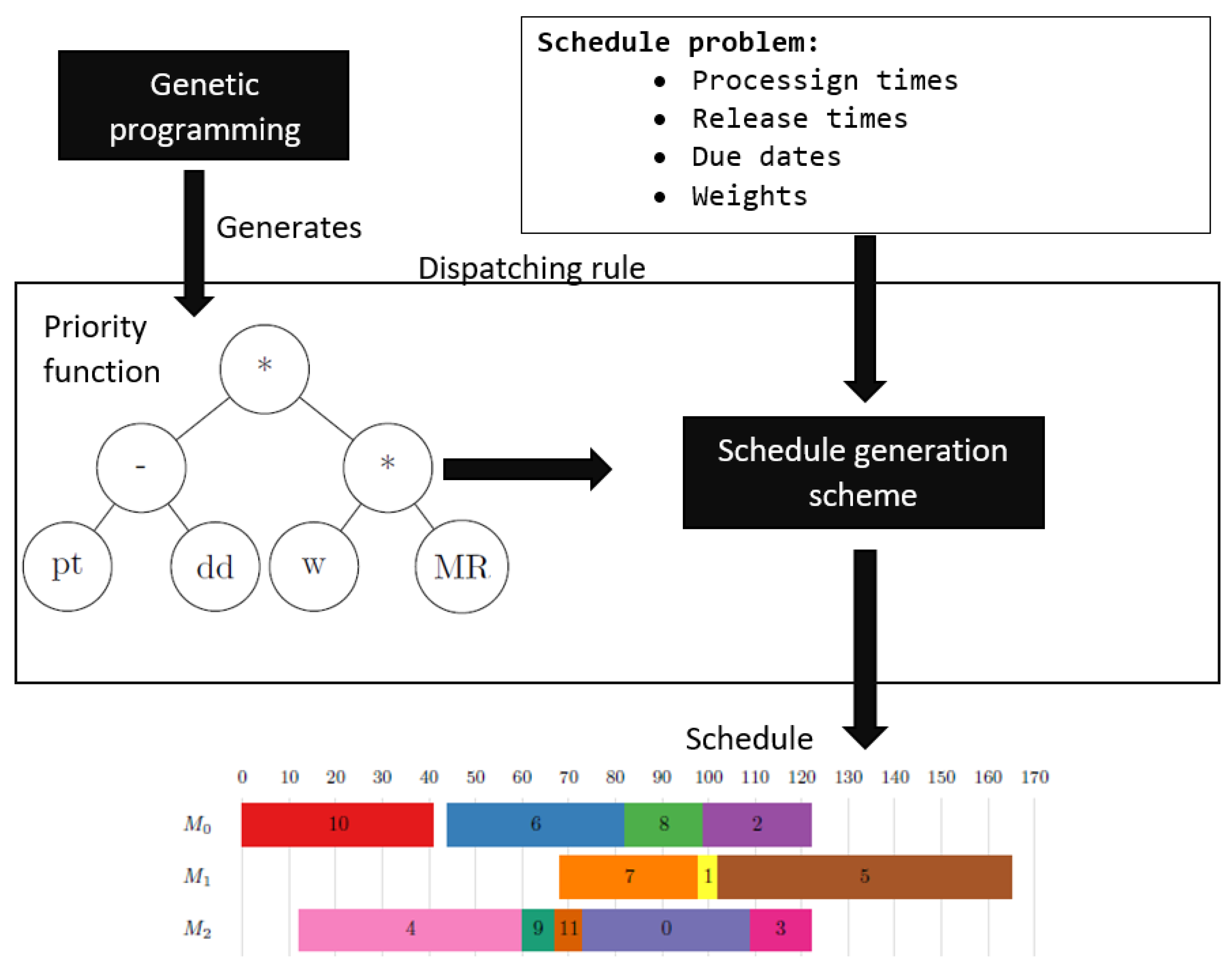
The entire methodology for the automatic creation of DRs is shown in
Figure 2. The figure shows that GP is used to generate PFs embedded in an SGS, as outlined in Algorithm 1. This combination represents a DR, which is then used to generate a schedule based on the characteristics of the scheduling problem (job processing times, due dates, etc.). The meaning of the symbols is outlined in
Table 1 and
Table 2. The schedule simply determines which job is assigned to which machine and the order in which they are executed on these machines. Finally, the quality of the created schedule can be evaluated using different performance criteria.
4. Methodology
As described in the previous section, the definition and selection of suitable terminal nodes is an important step in applying GP to develop new DRs. This is probably also the most difficult step, as it requires a certain amount of expert knowledge about the problem in order to define these terminal nodes in a meaningful way. However, even with good expert knowledge, there is no guarantee that the defined nodes will enable GP to obtain good priority functions. Therefore, the aim of this study is to investigate the process of designing the terminal set in more detail and determine how the inclusion and construction of different features and nodes affect the performance of GP.
This investigation is divided into three phases, each focusing on the influence of the following factors: (1) atomic terminal nodes, (2) composite terminal nodes constructed based on the frequency of occurrence in the previous phase, and (3) composite terminal nodes designed manually. In the following, we describe each phase in detail.
4.1. Atomic Terminal Nodes
In the first phase, only atomic terminal nodes, labelled in
Table 1, are used. These nodes are called atomic because they represent the most basic information about the problem at hand, such as the processing times of jobs, their due dates, weights, and so on. They cannot, therefore, be broken down into sub-expressions of simpler nodes or coded in any other way. GP can combine these nodes into more complex expressions that are interpreted as PFs to determine which scheduling decision should be selected at each decision point.
Even if the previously defined set of terminal nodes is sufficient to construct any complex expression, this might prove quite difficult for GP, since it is very likely that such expressions are easily perturbed by genetic operators. Therefore, it makes sense to define composite terminal nodes, i.e., nodes that are represented as a kind of expression computed from multiple atomic nodes. However, there are several ways to define compound terminal nodes, and these are analysed in the second and third phases of the study.
4.2. Frequency-Based Composite Terminal Nodes
In the second phase, we analyse whether it is possible to automatically construct new terminal nodes by using the frequency of occurrence of sub-expressions from previously developed PFs that work well. This phase is, therefore, based on the results of the first phase to determine which sub-expressions occur most frequently but only in the PFs with the best performance. From the best PFs, we calculate the frequency of occurrence of all sub-expressions and select the most frequent ones. We also define new terminal nodes that encode these sub-expressions and add them to the terminal set.
4.3. Manually Designed Composite Terminal Nodes
In the third phase, we investigate the influence of composite, manually designed terminal nodes that combine different basic information from
Table 1 in different ways. The motivation for introducing these terminals arises from several existing manually designed DRs that use similar information to that presented in
Table 2. For example, these nodes represent information such as the slack of the job, a feature often used in manually designed DRs developed to optimise the
criterion, or the time until a particular machine is available. Since such information has proven valuable in various manually created DRs, there is reason to believe that it could also be useful in the context of automatically created DRs. Therefore, we have investigated their influence on the performance of GP.
4.4. Feature Selection Methods
Although we have defined various terminal nodes, not all of them are equally useful for GP in designing new DRs. The problem with including unnecessary terminal nodes is that the solution space in which GP searches for a suitable PF increases exponentially. Therefore, it becomes increasingly difficult for GP to converge to good solutions. Therefore, it is not sufficient to define only a set of terminal nodes that represent all features of the problem; it is also crucial to determine whether these features are relevant for GP.
Although various algorithms and methods for feature selection have been defined in the literature [
59,
60,
61], we use two simple methods: backward sequential feature selection (BSFS) and frequency-based selection (FBS). Although simple, the BSFS method is commonly used in the machine learning community to select appropriate features. The reason we select only the above-mentioned methods is that our goal is to determine the best feature set for the problem under consideration rather than compare different feature selection methods.
BSFS starts with the complete feature set and removes one feature from the feature set in each iteration. GP is then executed with this reduced feature set, and the developed PFs are evaluated. The reduced set that results in the best performance for the generated DRs is selected, and the procedure is repeated until all features are removed. So, in each iteration, this method tests the effect of removing each feature on the results and removes the feature that has the least negative effect. This process requires a quadratic number of experiments to determine the appropriate terminal set.
The FBS method also starts with the complete feature set to generate a certain number of DRs. Based on the best DRs, the frequency of occurrence of each terminal node is determined. The node that occurs the least frequently is removed, and the process is repeated until all terminal nodes are removed from the terminal set. This method, therefore, removes the node that occurs least frequently in the generated PFs in each iteration. Compared to the BSFS method, this method only requires a linear number of experiments in relation to the terminal nodes. This is because only one experiment is performed in each iteration, on the basis of which the frequency of occurrence of terminal nodes can be determined to decide which node should be removed next.
6. Analysis
6.1. Comparison of Results from Each Phase
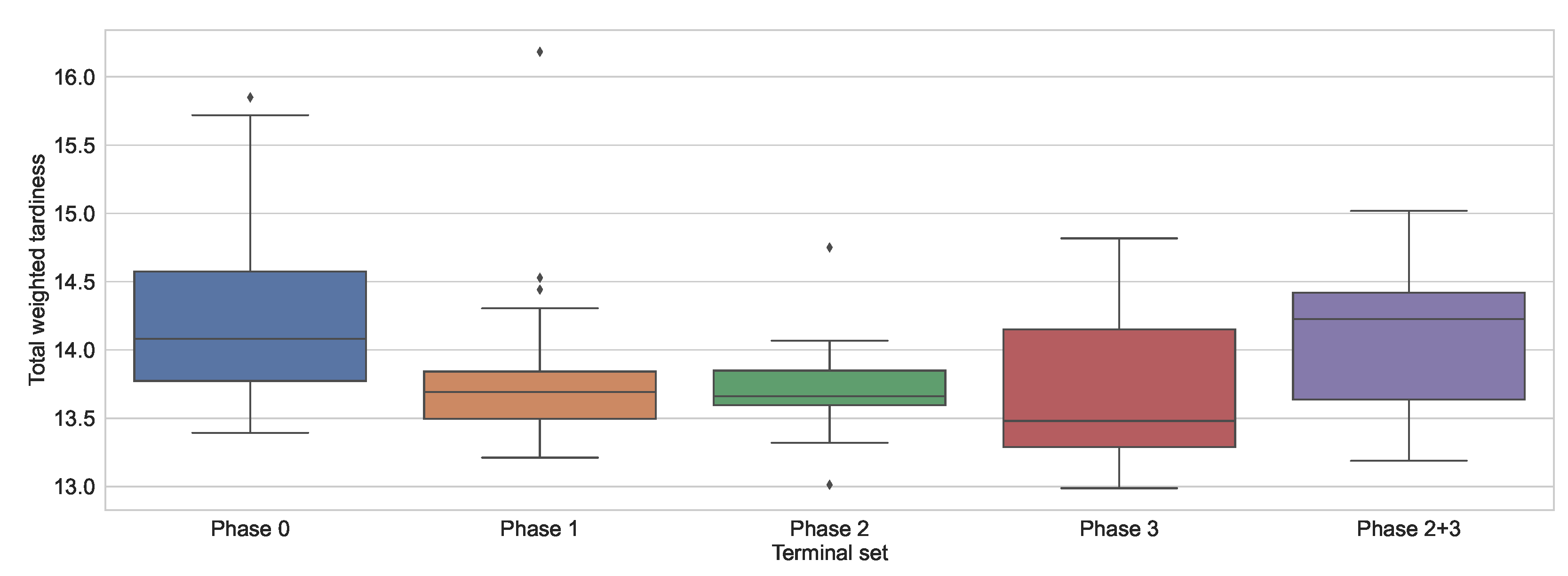
Table 11 gives an overview of the best results obtained with the validation set for each terminal set, as well as the best manually developed DRs, namely EDD, COVERT, and ATC. The initial feature set from
Table 1 is labelled as Phase 0, whereas Phase 2 + 3 refers to the combination of the best feature sets from Phase 2 and Phase 3, which was used to investigate whether the combination of these two feature sets led to an improvement in the results. In addition, the table shows the average rule size obtained when using each terminal set, which represents the average number of nodes in the expressions generated by GP. Compared to the manually generated DRs, we can see that GP achieved better DRs with the best terminal set obtained after each phase compared to the three manually generated ones. Only in the cases where no optimisation was performed, or when Phases 2 and 3 were combined, did GP fail to outperform the ATC rule. This shows that even for a terminal set with atomic terminal nodes, GP can reasonably combine them to outperform the existing rules. However, for more complex terminal nodes, GP can even increase the gap between manually and automatically created DRs.
Figure 3 depicts the results from
Table 11 as a box plot. The figure shows that the terminal node sets from Phase 1 and Phase 2 lead to the least scattered solutions. This is favourable, as it means that GP is more likely to produce a result close to the median. Therefore, the method is more reliable when it comes to generating solutions of expected quality. On the other hand, the solutions obtained when using the terminal node set obtained in Phase 3 are quite scattered. The results also show that GP is more likely to obtain better results with this terminal node set than with any other terminal node set.
To determine whether there was a significant difference between the results, the statistical tests described above were used, and a
p-value close to 0 was determined. This shows that there was a significant difference between the results obtained. To determine which of the results were significantly different, the post hoc test was used, the results of which are shown in
Table 12. The table shows that the results in the row are inferior to those in the column when indicated by “<”, superior when indicated by “>”, or equivalent when indicated by “≈”. We can see that the results obtained using only the atomic nodes, without optimising the terminal set, usually led to the worst results. In contrast, there was no significant difference between the results from Phases 1, 2, and 3.
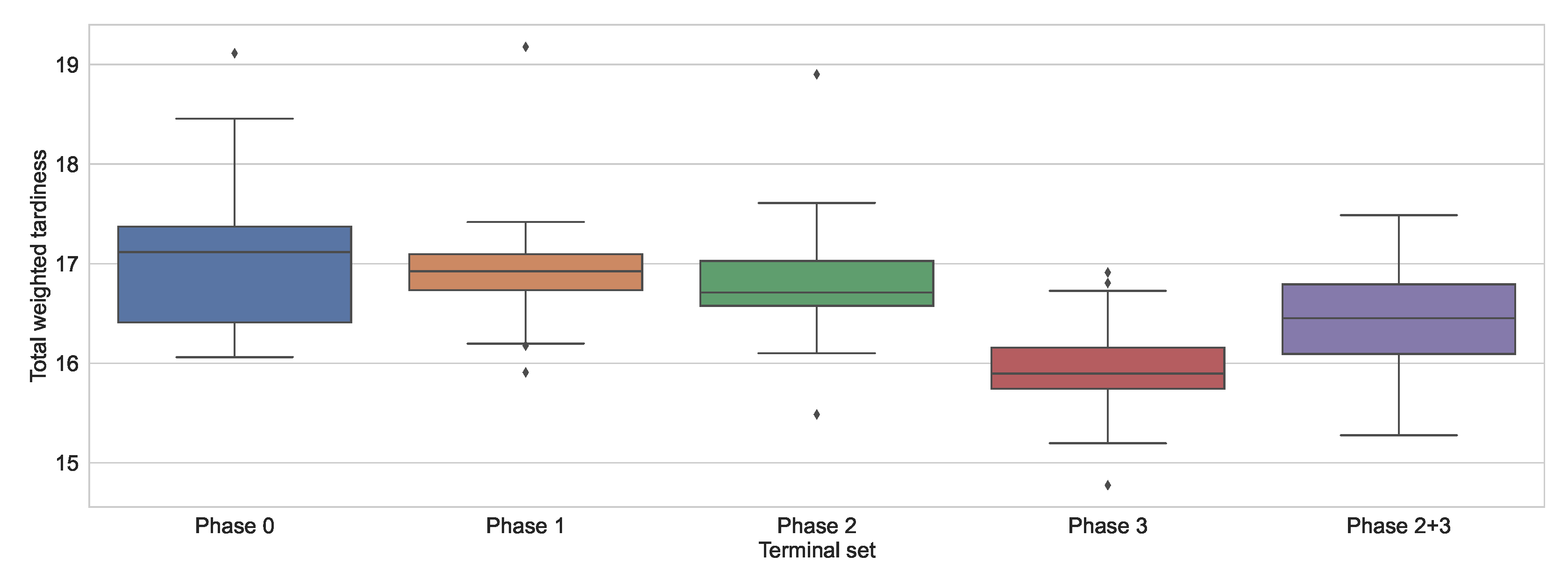
The above results summarise the validation set. In order to more objectively evaluate the performance of GP with the different terminal sets, the rules obtained were evaluated using the test set. These results are listed in
Table 13. It can be seen from the table that the performance of the rules obtained is now quite different from before. In this case, the results before feature selection only outperformed the simplest DR but not the two more complicated ones, namely COVERT and ATC. Even after Phases 1 and 2, GP could only find rules that performed similarly well to the manually designed rules. Only when the manually designed terminal nodes were finally introduced did GP generate rules that clearly outperformed the manually designed rules. The results are also shown as a box plot in
Figure 4 to better illustrate the differences between the results. The figure illustrates that the introduction of manually designed composite terminal nodes led to the greatest increase in performance.
To confirm that the addition of manually designed composite nodes led to a significant improvement in the results, the Kruskal–Wallis test was used, and a
p-value of 0 was obtained, meaning that there was a significant difference. The results of the post hoc tests performed are shown in
Table 14. The table shows that although in most cases there was no significant difference between the terminal sets, the use of manually designed composite terminal nodes significantly improved the results compared to those obtained in Phases 0, 1, and 2.
Based on the previous results, we can see that the manually designed terminal nodes actually provided the most valuable information about the problem, allowing the rules to generalise well to unseen problem instances. Presumably, all methods performed similarly on the validation set, as the best terminal sets were selected for them. However, it appears that this may have led to a slight overfitting to the validation set. Based on the previous observations, it is, therefore, safe to conclude that a mixture of simple and manually designed composite terminal nodes is required to create the best DRs.
6.2. DR Complexity Analysis
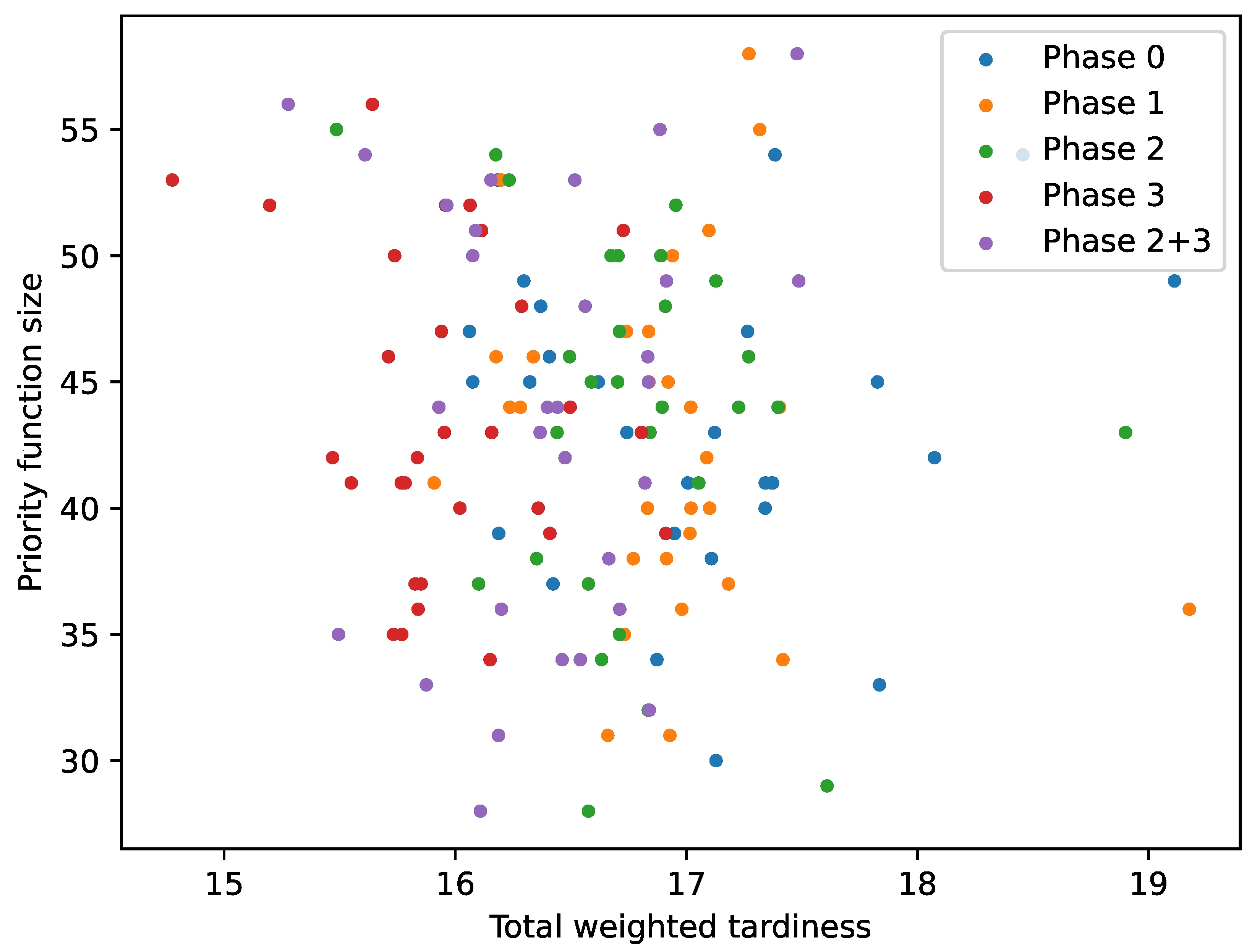
One could assume that a potential advantage of introducing composite features into the terminal set could be the generation of smaller expressions. To analyse this,
Figure 5 presents a scatter plot in which the fitness of the DR (x-axis) is plotted against its size (y-axis) for each terminal set used. The figure illustrates that the solutions are very widely scattered and only a very small number of rules below size 30 were obtained. Furthermore, the smaller rules usually did not perform well, often reaching a Twt value of over 16. It seems that the generated DRs started to perform well at around size 35. However, the best overall rule had a size of more than 50, and some other well-performing rules also had sizes of more than 50 nodes. To determine whether there was a correlation between the rule size and its performance, Spearman’s rho test was used. Since values between −0.15 and 0.1 were obtained for the results of all phases, we can conclude that there was no obvious correlation between these two measures. Although it may seem counterintuitive as to why smaller expressions were not obtained for composite terminal nodes, as more complex expressions should be represented by a smaller number of nodes, this was most likely due to the bloating of GP, and could be mitigated by using different mechanisms to control the bloating [
62,
63].
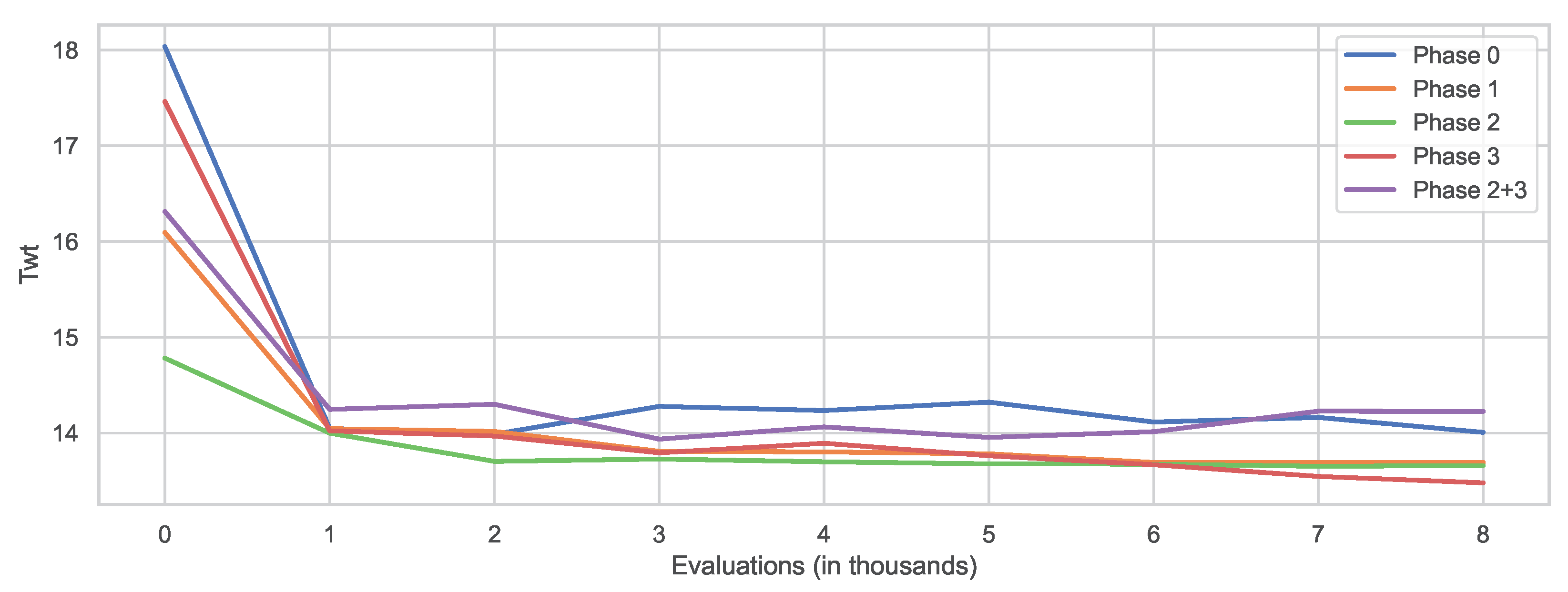
6.3. Convergence Analysis
Another interesting aspect to investigate is the rate of convergence of GP when using different terminal node sets. For this purpose, the best individual was saved after every 10,000 evaluations and later evaluated on the validation set. This was done for all 30 executions, and the median values were calculated and then used to plot
Figure 6. The figure illustrates that the terminal set significantly influenced the quality of the initial solution. The worst solution quality was obtained either with the initial terminal set (Phase 0) or the one obtained from Phase 2 + 3. The reason for this could be that these terminal node sets were larger and, therefore, it was more difficult for GP to generate a good initial solution. Interestingly, the terminal set from Phase 2 achieved the best initial solution, indicating that the
node used contributed to the development of good solutions. Moreover, this terminal led to the fastest convergence of the algorithm in the first half of the evolutionary process, although the algorithm started to stagnate after a certain time. When using the terminal set obtained in Phase 3, GP started with quite poor solutions; however, in the end, it reached the best overall solutions. This suggests that this terminal set might have been the most meaningful, and GP was thus able to produce high-quality DRs. However, it also seemed to be much more difficult for GP to obtain these solutions, thus requiring a longer evolution process, as it can be seen that the quality of the solutions themselves had improved by the end of the assigned number of scores. Therefore, there is a possibility that with more time, GP could achieve even better solutions with this terminal set.
6.4. Removal-Sequence Similarity
To analyse how similar the order in which the terminal nodes were removed from the terminal set was, the Levenshtein distance measure was used to determine the similarity of the two removal sequences. For this purpose, the removal sequences of BSFS and FBS were determined, and the Levenshtein distance for these two sequences was calculated for each phase. The Levenshtein distance values obtained, scaled between 0 and 1, were 0.666, 0.571, and 0.666 for the removal sequences obtained in Phases 1, 2, and 3, respectively. The values obtained show that there were indeed large differences between the removal sequences of the two selection methods. Thus, even if FBS could determine the nodes to be removed, it still deviated significantly from the sequence obtained by a more thorough search for the optimal feature set.
6.5. Run-Time Analysis
In this section, we briefly analyse the running times of the two feature selection algorithms. The complexity of FBS is linear with the number of features, i.e., to determine the best set of terminals,
experiments must be performed, where
N denotes the number of features. The
appears because it is not necessary to perform the last experiment with only a single feature. On the other hand, BSFS has a quadratic complexity and requires about
experiments. This obviously represents a significant difference in execution time, as the execution time of GP for the 80,000 fitness evaluations was about 1 h. Thus, in the case where nine terminal nodes were included in the set, FBS required 8 experiments, whereas BSFS required 44. Since each experiment was executed 30 times, and each execution took 1 h, FBS was executed for a total of 240 h, whereas BFSF was executed for 1320 h. It is assumed that all experiments are run in series. However, in many cases they can be run in parallel, reducing the total execution time. Although a smaller number of evaluations could be used, this would likely lead to a degradation in performance, as previous studies have shown that GP performs best for the given number of feature evaluations [
16].
7. Conclusions and Future Work
The aim of this study was to investigate the impact of different types of terminal nodes on the performance of GP in developing DRs for unrelated machine scheduling problems. The experimental results show that when GP is equipped with only atomic features to generate DRs, it can outperform simple DRs but has difficulty in evolving rules better than complex manually designed DRs. Therefore, two methods were used to construct composite terminal nodes and improve the performance of GP. In the first method, new terminals were constructed based on sub-expressions most commonly found in DRs developed with atomic terminals. Although with these terminals, GP matched the performance of manually constructed DRs, it still rarely outperformed them. However, the second approach, where composite terminal nodes were designed manually, proved to be more efficient and allowed GP to generate DRs that significantly outperformed manually designed DRs. Therefore, a certain level of expertise is required when designing terminal nodes, as it is necessary to define terminal nodes that provide more complex information about the scheduling problem. In addition to defining new terminals, it is also imperative to apply a feature selection method to determine the appropriate set of terminal nodes to prevent the search space from growing exponentially. The experiments showed that selecting terminal nodes based on their frequency of occurrence can help in selecting meaningful terminal nodes. However, this approach is not as robust as standard feature selection methods, such as backward sequential feature selection.
The results obtained in this study open up several avenues for future research. One possible research direction, which was only briefly explored, would be to introduce feature construction methods into the GP algorithm so that it can automatically design new features. In addition, better measures for identifying relevant features and sub-expressions are needed, aside from frequency of occurrence. Finally, another option would be to manually construct additional terminal nodes, as such nodes usually lead to better results compared to those constructed based on the frequency of occurrence.


