New Insights into Fuzzy Genetic Algorithms for Optimization Problems

Abstract

In this paper, we shed light on the use of two types of fuzzy genetic algorithms, which stand out from the literature due to the innovative ideas behind them. One is the Gendered Fuzzy Genetic Algorithm, where the crossover mechanism is regulated by the gender and the age of the population to generate offspring through proper fuzzy rules. The other one is the Elegant Fuzzy Genetic Algorithm, where the priority of the parent genome is updated based on the child’s fitness. Both algorithms present a significant computational burden. To speed up the computation, we propose to adopt a nearest-neighbor caching strategy. We first performed several experiments, using some well-known benchmark functions, and tried different types of membership functions and logical connectives. Afterward, some additional benchmarks were retrieved from the literature for a fair comparison against published results, which were obtained by means of former variants of fuzzy genetic algorithms. A real-world application problem, which was retrieved from the literature and dealt with rice production, was also tackled. All the numerical results show the potential of the proposed strategy.

1. Introduction

Fuzzy genetic algorithms (FGAs) are kinds of genetic algorithms (GAs) that employ fuzzy logic (FL) at some point in the process of mutation, crossover, selection, or updating the hyperparameters. The fuzzy reasoning has been exploited by several authors for the complex problem of dynamic control of GA parameters. There is ample literature devoted to the application of FGAs, e.g., in security [1,2], engineering [3,4], web applications [5], and manufacturing [6]. Despite the numerous articles of this type, there are not so many that introduce variants of FGAs. In [7], the authors proposed FL-controlled GAs, where mutation and crossover probabilities were dynamically adjusted by FL controllers. The application problem they considered was simulations of economic dispatch and emission dispatch. In [8], the authors presented dynamically controlled GA simulations, with population size and mutation and crossover rates adjusted using the FL controller. Inputs to the controller were genotypic diversity and phenotypic diversity, and outputs of the controller were population size change, mutation rate change, and crossover rate change. At any rate, in [9], it was stated that using a population diversity metric in an FGA can significantly improve premature convergence. Input variables of the fuzzy controller were population diversity, average population diversity divided by the maximum population diversity, and the number of unchanged greatest fitness values. As in some of the previously reviewed works, authors used mutation and crossover probabilities as output variables. An improved version of the FGAs in [8] was presented in [10], modifying some fuzzy inference rules and introducing a scaling factor for normalizing the input variables. In [11], a GA with varying population size (GAVaPS) was enhanced with a fuzzy logic controller by adapting the crossover probability according to a fuzzy rule base. The resulting method was called fuzzy-based lifetime extended GA (LTexGA). A hybrid fuzzy genetic algorithm (HFGA) was developed in [12]. In this FGA variant, the average fitness value and the best fitness value of each generation were adopted for the dynamical tuning of the crossover and mutation probabilities. The HFGA was used to tackle the problem of an optimal grouping of tank crews, based on training time, qualifications, and specialization of soldiers. The authors of [13] tried to improve the adaptive method of [10]. In the proposed improved fuzzy genetic algorithm (IFGA), the average fitness value and standard deviation changes between two consecutive generations were selected as the input variables, using two adaptive scaling factors to normalize the input variables. An interesting variant of FGA was introduced in [14] a few years later. The authors proposed a gendered fuzzy genetic algorithm (GFGA), i.e., GA with gendered selection based on fuzzy rules and age/lifetime formulas. GFGA was successfully used to generate the weights of a neural network (NN). More recently, the elegant fuzzy genetic algorithm (EFGA) was proposed [15] with a min-heap data structure for prioritizing genomes for the optimization of the initial weights of complex-valued NNs. In the EFGA, mutation rate, crossover rate, and reproductive group size were updated using fuzzy rules. In [3], the authors introduced a bilinear fuzzy fitness function in a standard GA to design optimal diagrid structures for tall buildings under engineering design constraints. In [2], the population selection was based on fuzzy clustering, with no explicit mention of fuzzy rules.

Here, we focus on FGAs using fuzzy rules. GAs remain largely unexplained to the end-user in terms of their search properties. An attempt to make GAs explainable was made by using surrogate models, which gave a partial understanding of the solutions limited to a single generation [16]. Needing to be trained, such a model comes with an additional computational cost. Fuzzy rules for controlling the GA’s search properties bring an enormous advantage: they can add explainability.

At any rate, in all the cited articles, the computational effort has not been properly discussed. Here, we consider the most recent fuzzy-rule-based variants of GAs, i.e., EFGA, along with GFGA, with the latter conceived in a very different way with respect to the other FGAs. We compare their performance on a set of benchmarks, noticing that there is no comparative analysis of the two in the literature. In fact, these kinds of FGAs were originally introduced as part of a learning algorithm of some type of NN. Here, the aim is not to replicate such applications but to explore the use and possible enhancement of the EFGA and GFGA for more general optimization problems. We discuss a possible strategy to speed up the fuzzy inference in these FGA variants. Such a strategy is inspired by nearest-neighbor caching (NNC), which is well known in the context of web applications [17] and wireless networks [18], but, to the best of our knowledge, was never applied to any specific case.

Some preliminary experiments on some well-known benchmarks were performed. The outcome of such experiments is that the results obtained by using the NNC are sufficiently accurate without any losses in performance and give a speed-up of over 90%, thus making it a viable alternative. For a fair comparison against former variants of FGAs, some case studies were retrieved from the literature, which include Dejong’s functions [19] and the traveling salesman problem (TSP) [11], thus confirming the good performance of the approach. Additionally, a real-world application problem related to rice production was investigated following the model and the GA results discussed in [20].

The contribution of the paper can be summarized as follows:

• An NNC strategy is discussed as a way to significantly speed up the fuzzy inference in two promising FGAs, from the explainability perspective, i.e., GFGA and EFGA, without any performance losses;
• Variants of the original GFGA and EFGA, in terms of fuzzy logic settings, are explored;
• A comparison against traditional and state-of-the-art techniques, which are both fuzzy and non-fuzzy, is presented over benchmark cases and a real-world application problem.

The paper is structured as follows. The next section is devoted to recalling some notions on fuzzy sets and the two considered FGA variants, i.e., EFGA and GFGA. In Section 3, the NNC strategy is described. Section 4 deals with the numerical experiments and discussion. Finally, some conclusions close the paper.

2. Fuzzy Genetic Algorithms: Dealing with Individuals and Fitness

In this section, we briefly present the considered FGAs, along with a few preliminaries.

2.1. Preliminaries

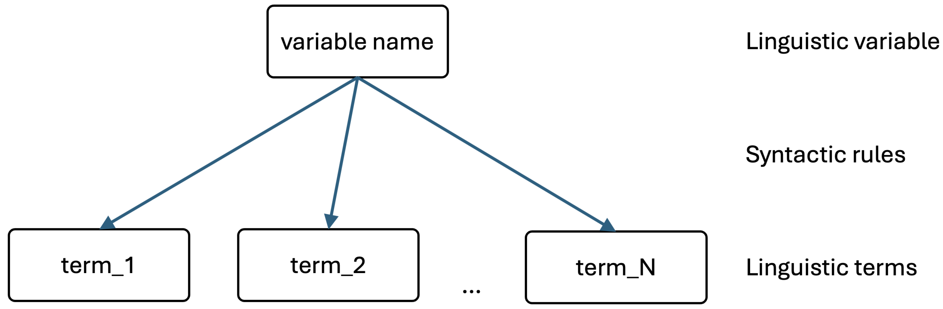
2.1.1. Fuzzy Sets

A fuzzy set generalizes the classical set, allowing not only for the classical set’s 0–1 membership degrees but also a continuum of values in the range [0, 1]. A fuzzy set A is uniquely defined over a universe of discourse U by a membership function (MF) $\mu$, ${\mu }_A:U\to [0,1]$. A fuzzy set is normal when its highest membership degree equals 1.

The most common MF is the triangular function. Another popular option is the trapezoidal MF:

$$\mu \left(x\right)=\left\{\begin{array}{cc}0\hfill & \mathrm{if}x\le a\hfill \\ {\displaystyle \frac{x-a}{b-a}}\hfill & \mathrm{if}a\le x\le b\hfill \\ 1\hfill & \mathrm{if}b\le x\le c\hfill \\ {\displaystyle \frac{d-x}{d-c}}\hfill & \mathrm{if}c\le x\le d\hfill \\ 0\hfill & \mathrm{if}d\le x\hfill \end{array}\right.$$

(1)

which models the linguistic expression “approximately b to c” or “close to [b, c]”. Dealing with a central interval (i.e., [b, c]), instead of a point as for the triangular MF, this type of MF allows to take into account a higher level of uncertainty.

It is worth recalling the pi-shaped MF:

$$\mu \left(x\right)=\left\{\begin{array}{cc}0,\hfill & \mathrm{if}x\le a\hfill \\ 2{\left({\displaystyle \frac{x-a}{b-a}}\right)}^2,\hfill & \mathrm{if}a\le x\le {\displaystyle \frac{a+b}{2}}\hfill \\ 1-2{\left({\displaystyle \frac{x-b}{b-a}}\right)}^2,\hfill & \mathrm{if}{\displaystyle \frac{a+b}{2}}<x\le b\hfill \\ 1,\hfill & \mathrm{if}b<x\le c\hfill \\ 1-2{\left({\displaystyle \frac{x-c}{d-c}}\right)}^2,\hfill & \mathrm{if}c<x\le {\displaystyle \frac{c+d}{2}}\hfill \\ 2{\left({\displaystyle \frac{x-d}{d-c}}\right)}^2,\hfill & \mathrm{if}{\displaystyle \frac{c+d}{2}}<x\le d\hfill \\ 0,\hfill & \mathrm{if}x\ge d\hfill \end{array}\right.$$

(2)

which represents a smoother alternative to the trapezoidal MF.

The connectives from the classical logic AND, OR are generalized in fuzzy logic via t-norms and t-conorms, respectively. A typical t-norm is the minimum operator, and a typical t-conorm is the maximum operator.

A fuzzy partition can be seen as a series of m partially overlapping normal fuzzy sets with $m\ge 2$. Such fuzzy sets represent the terms of a linguistic variable. For instance, the linguistic variable temperature may have the terms {cold, cool, warm}, each one expressed by a fuzzy set, i.e., a proper membership value. As in our natural language, the terms represent the attributes of the linguistic variable. Any linguistic variable can assume a certain value, i.e., membership degree, which has relevance in fuzzy IF-THEN rules. Figure 1 recalls the generic N terms of a linguistic variable (here denoted as term_1,…,term_N), determined by syntactic rules to form eventually fuzzy rules. Examples of fuzzy rules will be provided in the next sections.

2.1.2. Genetic Algorithms

Natural evolution is the source of inspiration for GAs, and typical evolutionary terminology can be found through the algorithm. One might think of the optimization problem as the environment and the proposed solution as a single entity inside it. Individual fitness is correlated with the quality of the candidate solution as determined by the objective function. The population is first randomly initialized by the algorithm, which then iterates through generations. Every individual in a generation is assessed for fitness, and new individuals (offspring) are produced depending on that evaluation. By applying mutations or merging parents (crossover), a new population is created.

2.2. EFGA

In EFGA, as in traditional GAs, an initial set of individuals is randomly generated. The approach relies on a min-heap data structure keyed at fitness in order to reduce the number of fitness function calls. The min-heap data structure is a binary tree, where each node is associated with a pair of numbers, i.e., the index assigned to the chromosome as a unique identifier and the fitness value. A simple example of min-heap is shown in Figure 2 where the integer in any node represents the above-mentioned index and the other value is the fitness value. The solutions that show minimal fitness are put on top levels of the tree, and they are more likely to be selected. The root presents the best solution. The algorithm is stopped when either the difference between the best and worst solution is below a certain threshold value (e.g., 0.003) or when the number of iterations exceeds the maximum iterations. Additionally, a large initial population is created to increase the likelihood of being close to local minima early on. However, large populations also have a lot of low-quality solutions. The authors of the original approach refer to the Pareto front by allowing only the top 20% of the individuals to reproduce.

In EFGA, fuzzy rules are used to update the simulation parameters. Average fitness, best fitness, and average fitness change are used as inputs. The first two variables are associated with the term set {Excellent, Acceptable, Poor}, and the last one with the term set {Low, Medium, High}. Crossover rate and mutation rate may take the linguistic values {Low, Medium, High}, while reproductive group size may take {Low, Medium, Large}. Fuzzy rules are also used for priority updates. After evaluating a child’s genome fitness, the parent genome priority is updated. Linguistic values for the child’s genome fitness are {Excellent, Acceptable, Poor}, the term set for the priority is {Very Low, Low, Medium, High, Very High}. Let $N_{priority}$ and $N_{fitness}$ be the number of terms of priority and fitness, respectively. We notice that $N_{priority}=2N_{fitness}-1$.

Remark 1.

We observe that the term sets for fitness and priority, respectively, could include more attributes as follows:

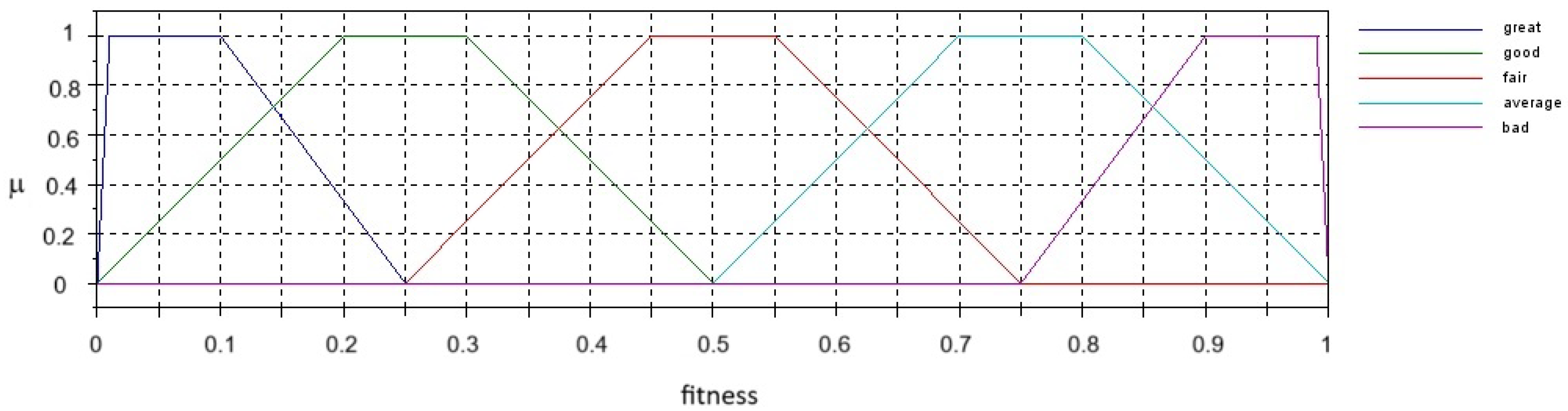
• {Great, Good, Fair, Average, Bad} and {Very Low, Low, Moderate, Medium, High, Very High, Extremely High, Exceptionally High, Extraordinary}, i.e., $N_{fitness}=5$;
• {Exceptional, Great, Good, Average, Mediocre, Poor, Terrible} and {Very Low, Low, Moderately Low, Below Average, Average, Above Average, Moderate, High, Very High, Extremely High, Exceptionally High, Extraordinary, Exceptional}, i.e., $N_{fitness}=7$;

having increased the linguistic attributes of priority proportionally.

An example of a fitness linguistic variable, with five terms expressed as trapezoidal MFs, is shown in Figure 3. In the original method, triangular MFs were adopted, but here we investigate trapezoidal MFs, in addition to pi-shaped MFs, as they allow for a higher degree of uncertainty, as explained in Section 2.1.1.

The rules are of the form

IF f1 IS term_i AND f2 IS term_j THEN priority is term_(2N-i-j-2)

• where $f1$ and $f2$ are the fitness of the parent genomes.

The goal is to move parent genomes with offspring having better fitness higher in the priority queue and parent genomes with worse offspring lower in the priority queue.

Regarding diversity, some formulas are meant to preserve it, as explained in the following.

Let ${\rho }_1^{\left(k\right)}$, ${\rho }_2^{\left(k\right)}$ be two chromosomes in the kth generation. A crossover is performed by randomly selecting two positions ${\overline{p}}_1,{\overline{p}}_2\in (0,1]$, with ${\overline{p}}_1<{\overline{p}}_2$.

The crossover operation is performed according to the following:

$$\begin{array}{ccc}\hfill {\rho }_1^{(k+1)}({\overline{p}}_1,{\overline{p}}_2)& =& \gamma {\rho }_1^{\left(k\right)}({\overline{p}}_1,{\overline{p}}_2)+(1-\gamma ){\rho }_2^{\left(k\right)}({\overline{p}}_1,{\overline{p}}_2)\hfill \end{array}$$

(3)

$$\begin{array}{ccc}\hfill {\rho }_2^{(k+1)}({\overline{p}}_1,{\overline{p}}_2)& =& (1-\gamma ){\rho }_1^{\left(k\right)}({\overline{p}}_1,{\overline{p}}_2)+\gamma {\rho }_2^{\left(k\right)}({\overline{p}}_1,{\overline{p}}_2),\hfill \end{array}$$

(4)

where ${\rho }_i^{\left(j\right)}({\overline{p}}_1,{\overline{p}}_2)$, with $i=1,2$, and $j=k,k+1$, represents a subchromosome, from position ${\overline{p}}_1$ to ${\overline{p}}_2$, and $\gamma \in [-1,1]$. As the crossover is performed on the subchromosome, the latter is (randomly) altered while some parent’s genes are retained. This helps with diversity.

2.3. GFGA

The original method splits the whole population into two groups with different genders. While in standard GAs, a crossover between any two individuals is possible, in the GFGA, this is possible only for opposite-gender individuals, as it works in nature. Moreover, selection rules are entirely different for male and female genomes. Some male genomes are randomly selected and matched with female genomes based on population diversity and male genomes’ age via fuzzy rules. Each genome has an age, which is simply the number of iterations that have passed since its initialization. Selection is applied based on the maximum age of the individual; when its age is greater than the maximum age, the genome is removed from the population.

The linguistic variable age has four terms: {Infant, Teenager, Adult, Elderly}. The term set for the population diversity is {Very Low, Low, Medium, High}. At the selection stage, males are selected randomly, and the age of female partners is estimated based on the age of male partners and population diversity using fuzzy rules. Then, a partner with the age closest to the desired one is selected, and crossover is performed.

Remark 2.

The term set for age and partner age could be the following (where $N_{age}=N_{partner-age}$):

• {Infant, Child, Teenager, Adult, Elderly};
• {Newborn, Infant, Toddler, Child, Teenager, Adult, Elderly};

including more linguistic attributes.

Similarly, the term set for diversity could be the following:

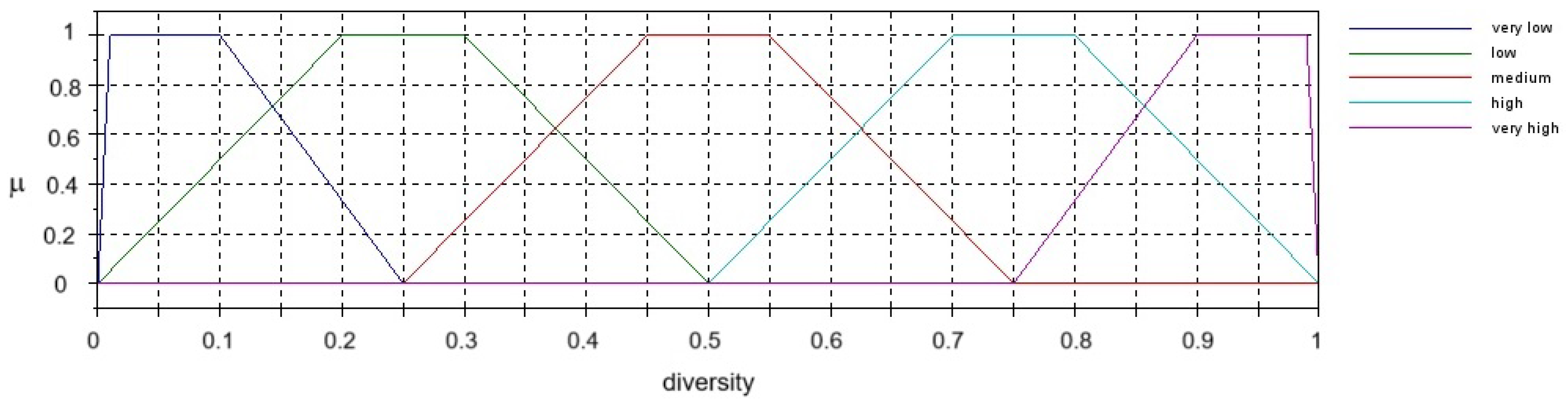
• {Very Low, Low, Medium, High, Very High};
• {Extremely Low, Very Low, Low, Medium, High, Very High, Extremely High};

Notice that for the highest age term, the second-highest age term for potential partners is prioritized if there is the highest diversity. With the lowest two diversity terms, there is the lowest age term for potential partners. Hence, the general rule can be written as follows:

    IF age IS term_i AND diversity IS term_j  THEN partner_age IS

    term_{2N-(i+j)+2}}

• except for the lowest diversity term or the highest age term and second-lowest diversity term:

    IF (age IS term_i AND diversity is term_1) OR (age IS term_N

    AND diversity IS term_2) THEN partner_age IS term_1.

Let us assume $N_{age}=N_{partner\_age}=N_{diversity}=5$, for example. Then the following rule is obtained:

    IF age IS adult AND diversity IS high  THEN partner_age IS adult

• since the index of the age and diversity terms is 4, resulting in an index for the partner age, which equals 4.

For $N_{age}=N_{partner\_age}=N_{diversity}=7$, a similar rule is obtained:

    IF age IS adult AND diversity IS very high THEN partner_age IS adult

• since the index of the age and diversity terms is 5, resulting in an index for the partner age, which equals 6.

For low and very low diversity, the following rule holds with $N_{age}=N_{partner\_age}=N_{diversity}=5$.

    IF (age IS adult AND diversity is very low) OR (age IS elderly

    AND diversity IS low) THEN partner_age IS infant.

Let m and M be the minimum and the maximum age in the population, and let n and P denote the population size and half of the population, respectively. The population diversity linguistic variable is defined as follows:

$$D_{pop}\left(P\right)=\left\{\begin{array}{cc}veryhigh\hfill & P\le L+t\hfill \\ high\hfill & m+t<P\le m+t+1\hfill \\ medium\hfill & m+t+1<P\le m+t+2\hfill \\ low\hfill & m+t+2<P\le m+t+3\hfill \\ verylow\hfill & P>m+t+3\hfill \end{array}\right.$$

(5)

where $t=\left[\lambda {\displaystyle \frac{m+M}{n}}\right]$, $\lambda =\left[{\displaystyle \frac{n}{10}}\right]$, with $[.]$ denoting the rounding operation returning the nearest integer number.

Figure 4 shows the diversity variable (5) with trapezoidal MFs.

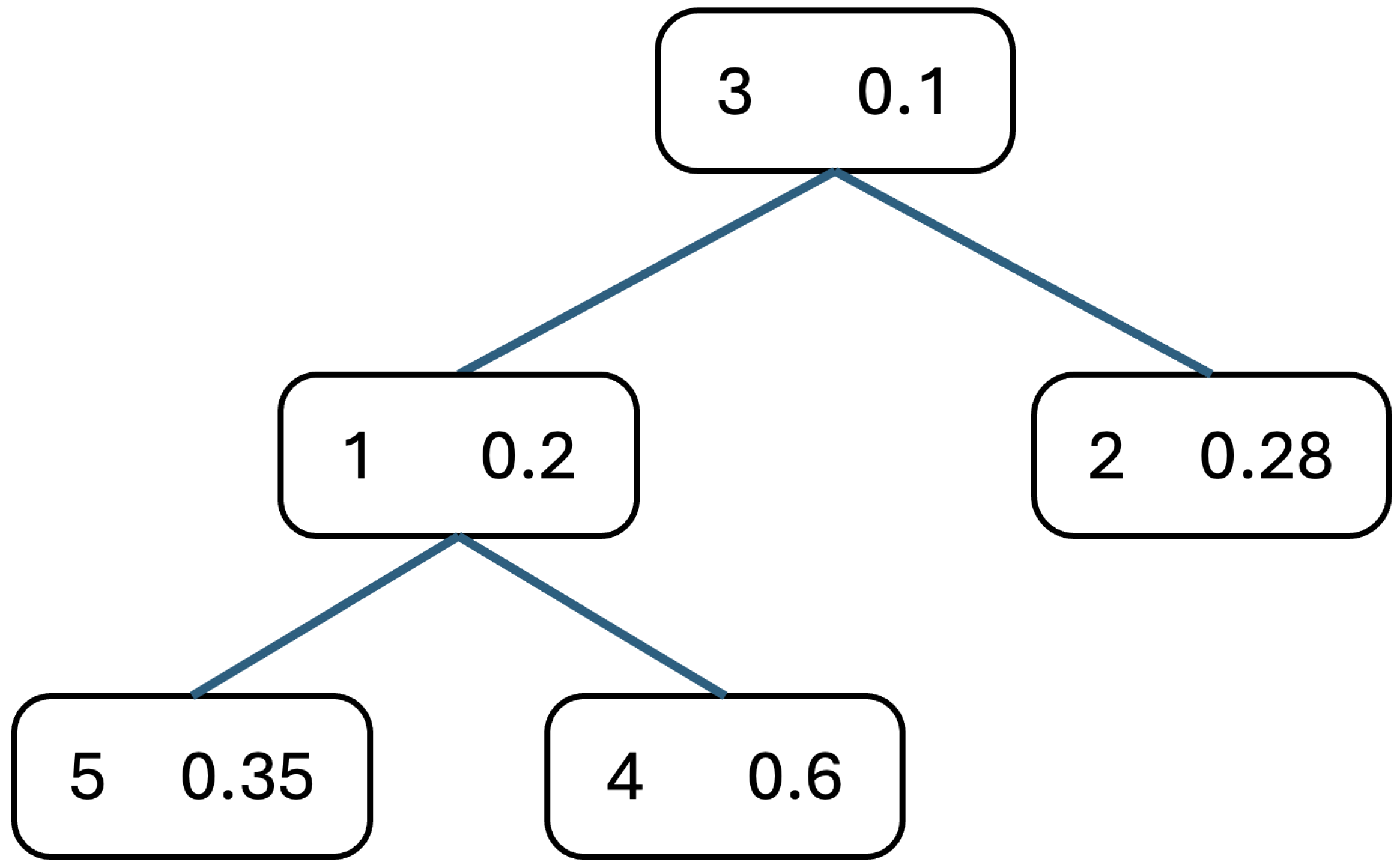
3. Nearest-Neighbor Caching

Here, we refer to caching as a technique to avoid repetitive computations thanks to some values stored in memory. Such values are retrieved when a function call with the same or similar inputs is needed. This may significantly reduce the runtime. Formally, there exists a metric space $(X,d)$ over the presented vector $\mathbf{x}$, and a threshold radius R. When a new vector $\overline{\mathbf{x}}$ (query) arrives, and if there is a stored vector $\mathbf{x}$ in the cache with $d(\mathbf{x},\overline{\mathbf{x}})\le R$, the request can be satisfied by the cache without any new computations. Let k be the size of the cache. It is expected that k increases as R tends to zero [21].

Operationally, the vector space is stored in a matrix. Distances from a query vector to the matrix rows are computed. A certain number of closest neighbors are selected, and their distances are stored. After finding k nearest neighbors, a weighted average of them is computed as an approximation of a certain function value:

$$\overline{g_i}=\sum _{i=1}^k{w}_i{g}_i,$$

(6)

where $g_i$ is a value of a function at the ith nearest point and $w_i\in [0,1]$ is a weight such that ${\sum }_{i=1}^k{w}_i=1$.

The weights of the nearest neighbors $w_i$ can be computed as normalized $L_2$ distances to the nearest neighbors $d_i$:

$$w_i={\displaystyle \frac{d_i}{{\sum }_{j=1}^N{d}_j}}.$$

(7)

For the remainder of this work, EFGA-NNC and GFGA-NNC will denote the implementation of the respective methods with NNC.

4. Experiments and Discussion

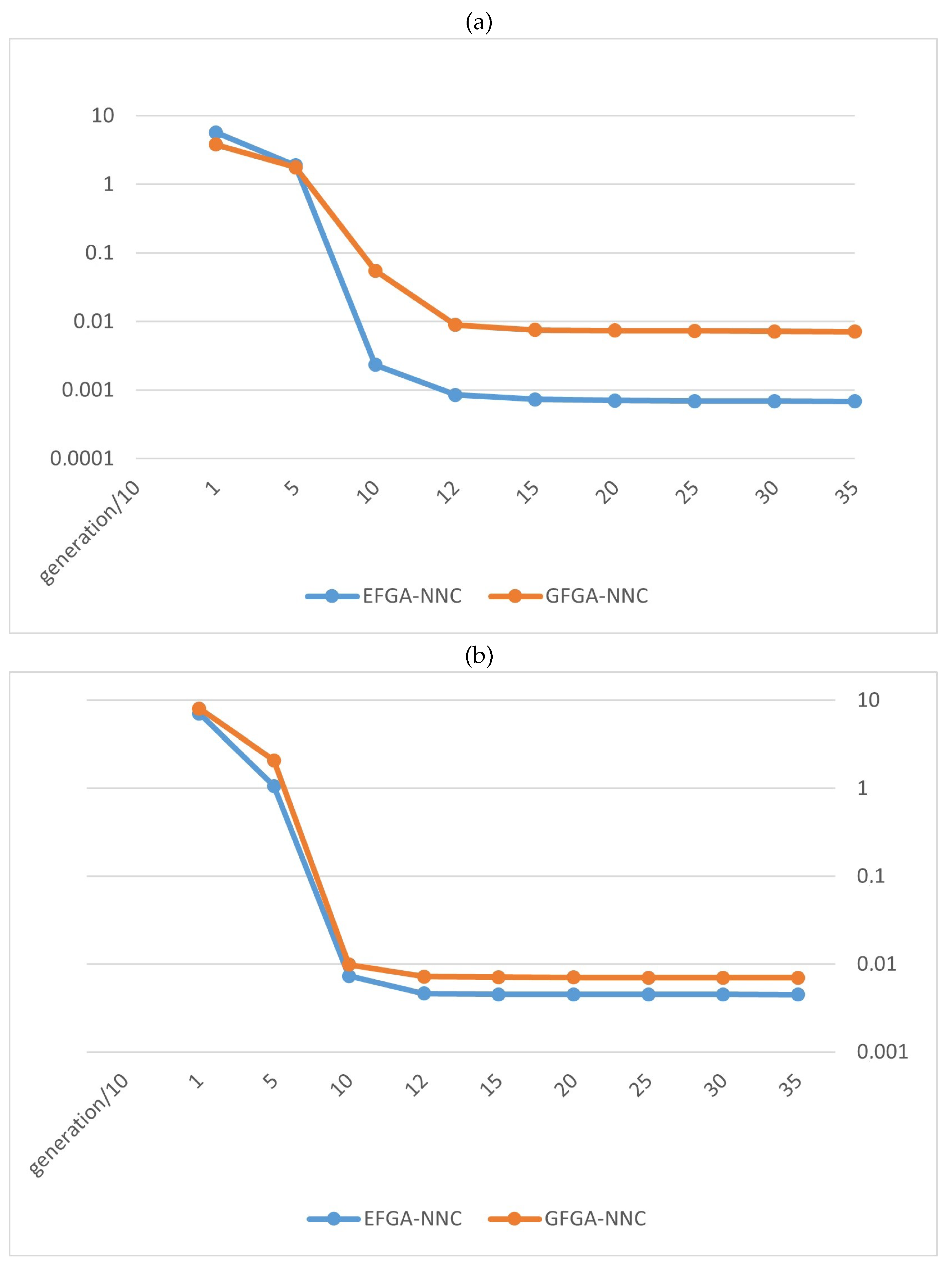
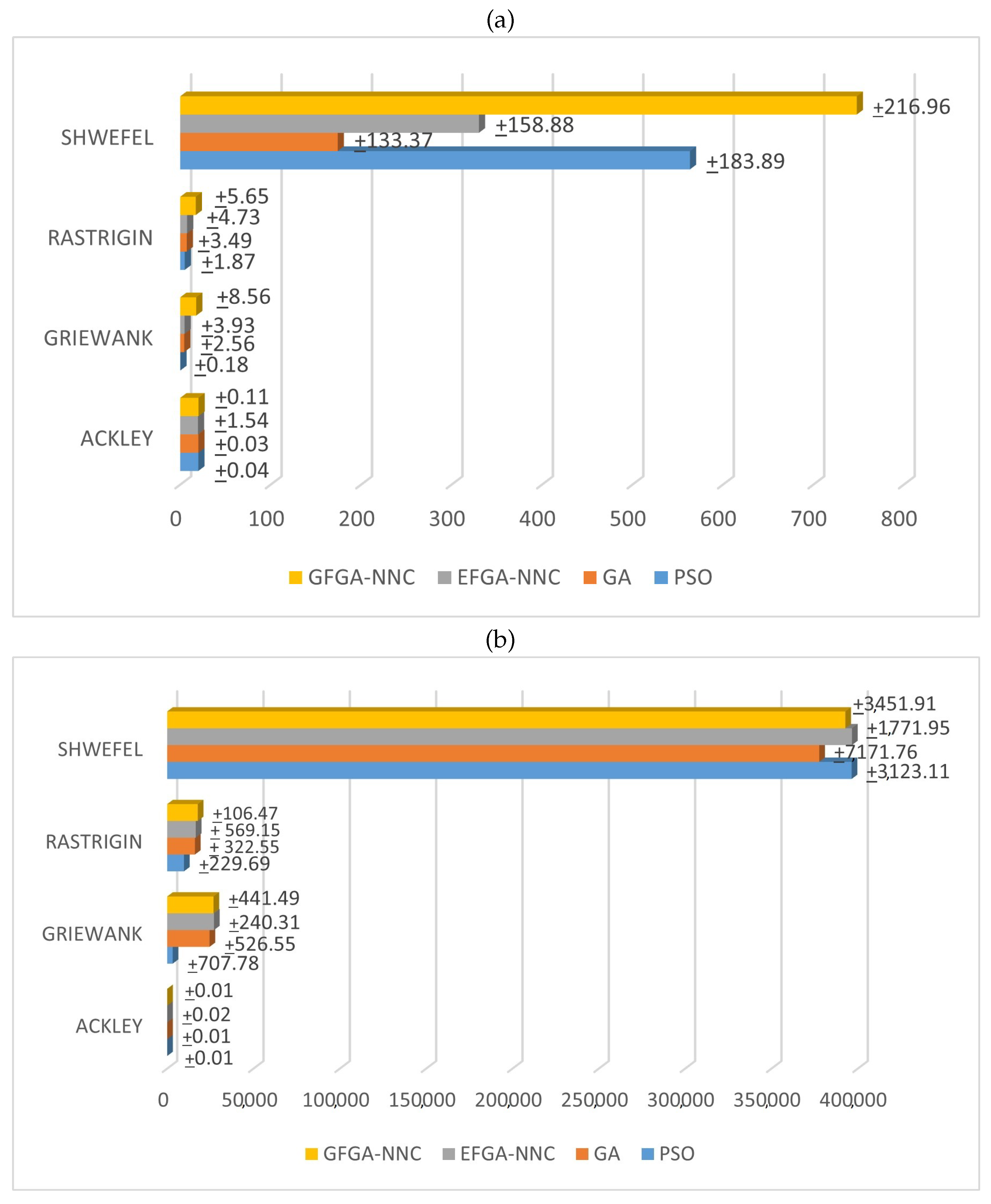
4.1. Initial Experiments on Popular Benchmarks

Experiments were run on the same initial population (ensured with the random seed) through 500 generations. The population size was 100, as in [15]. For any considered benchmark function, there were 20 runs, considering two possible dimensions, i.e., $D\in \{5,1000\}$. The minimum type t-norm and the product type t-norm were considered. Similarly, the maximum type and the sum type t-conorm were employed. Regarding the membership functions (MFs), two options were explored, i.e., pi-shaped and trapezoid. The aim here was to explore variants of the original EFGA and GFGA, where only the triangular MFs and the minimum t-norm were used.

For EFGA, it was chosen $N_{fitness}=\{3,5,7\}$. The same values for $N_{age}$ are in GFGA. A larger number of terms would not be beneficial for interpretability.

Four typical benchmarks for algorithms in optimization tasks were considered:

• The Schwefel function

  $$f_1\left(\mathbf{x}\right)=418.9829d-\sum _{i=1}^D{x}_{i}sin\left(\sqrt{\left|x_i\right|}\right),x_i\in [-500,500],$$

  (8)
• The Rastrigin function

  $$f_2\left(\mathbf{x}\right)=10D+\sum _{i=1}^D\left(x_i^2-10cos\left(2\pi x_i\right)\right),x_i\in [-5.12,5.12],$$

  (9)
• The Griewank function

  $$f_3\left(\mathbf{x}\right)=\sum _{i=1}^D{\displaystyle \frac{x_i^2}{4000}}-\prod _{i=1}^{D}cos\left({\displaystyle \frac{x_i}{\sqrt{i}}}\right)+1,x_i\in [-40,40],$$

  (10)
• The Ackley function

  $$f_4\left(\mathbf{x}\right)=-a{e}^{\left(-b\sqrt{{\displaystyle \frac{1}{D}}{\sum }_{i=1}^D{x}_i^2}\right)}-e^{\left({\displaystyle \frac{1}{D}}{\sum }_{i=1}^{D}cos\left(c{x}_i\right)\right)}+a+e,x_i\in [-32.768,32.768].$$

  (11)

The choice of the benchmark functions and the dimension has been motivated by the presence of relevant results in the literature, as will be discussed in the following.

The different MFs did not affect the results significantly: a difference of less than 5% on average was observed. Regarding t-norm or t-conorm types, we observed that the best results were obtained by using the combination of min t-norm and max t-conorm, and this combination was kept for the rest of the experiments, including those discussed in the next sections. We observed that the results between the two types of implementation (i.e., the original one and that with NNC) had no significant differences, i.e., not greater than 3%. Similarly, assuming $N_{fitness}>5$ for EFGA-NNC and $N_{age}>5$ for GFGA-NNC did not produce any significant changes in the results and even worsened them. Regarding the MFs, we observed a slightly better performance by using pi-shaped MFs. Hence, we fixed it for all the remaining experiments. Instead, the NNC strategy allowed to significantly shorten the runtime. The same experiments with the same fitness function and parameters were run several times, as described before, and mean runtime and runtime standard deviation were compared. The ratio s between the runtime with and without NNC in the case of EFGA is $s=0.077\pm 0.022$ and $s=0.014\pm 0.007$ for GFGA. Comparing the runtime of EFGA-NNC and GFGA-NNC to that of the standard GA, the latter is still more competitive, with 30–50% shorter runtimes on average, where the worst case is the high-dimensional one (i.e., D = 1000). This computational burden may be seen as the cost of explainability [16].

The results using the different techniques are depicted in Figure 5a,b. Both for $D=5$ and $D=1000$, there is no significant difference between the results by EFGA-NNC and GAs, except for the case of the Shwefel function. In that case, the GA outperforms the other approaches, especially for $D=5$. At any rate, the advantage over the standard GA is boosting explainability. Regarding the GFGA-NNC, it performs better for problems with higher dimensions, being comparable to the other approaches. The PSO outperforms the other approaches for the Rastrigin and Griewank functions. There is no significant difference among all the approaches in the case of the Ackley function, both for $D=5$ and $D=1000$. In all the cases, except for the Ackley function, with any dimension, the highest standard deviation was observed for the GFGA-NNC. For the EFGA-NNC, it was found that the standard deviation was generally comparable to that related to the GA or even less in a couple of cases (both for D = 5 and D = 1000), suggesting better stability of the EFGA-NNC with respect to the GFGA-NNC.

The $f_2$ function, with $D=5$, was also considered in [22] and the results by a fuzzy logic controlled genetic algorithm (FCGA) [7], an improved fuzzy genetic algorithm (IFGA) [13] and another kind of FGA [23] were compared. The latter outperformed the other methods, providing an average fitness value of around 100 after 14 generations, while IFGA provided the closest value to the optimum in the least average number of generations, i.e., 1205. The authors used a population of 20 individuals. With the same population size and after 14 generations, we obtained 85 and 68 by GFGA-NNC and EFGA-NNC, respectively. In Figure 6a,b, one can see the effect of the type of MF, t-norm, and t-conorm on the result by EFGA-NNC, where $m=N_{fitness}$, for the sake of simplicity. One can observe that the best result was obtained by using the min t-norm and max t-conorm (max-min on the plot). Even though there is not much difference due to the type of MF, it is possible to see that the best result was obtained with $m=5$ and pi-shaped MF. Similar behavior was observed over the other benchmarks.

The benchmark functions $f_1$, $f_2$, and $f_4$ with the same domains and $D=1000$ have been considered in [24], where the same number of runs was also adopted (i.e., 20). The authors of [24] used a standard GA as a baseline but with a population size of 50 and a number of iterations of 1000. They performed the experiments with their approach, i.e., the adaptive dimensionality reduction genetic algorithm (ADRGA), the hybrid genetic and simulated annealing algorithm (HGSA), and the adaptive genetic algorithm (AGA). We consider their published results for a fair comparison, reporting our results after 1000 generations. In Figure 7, the mean and standard deviation (sd) for the above-mentioned benchmark functions are shown. For the Ackley function, the results by EFGA-NNC and GFGA-NNC are quite close to that by ADRGA, also considering that the standard deviation for the latter is 20 times greater than that of EFGA and GFGA. A similar situation can be observed for the Shwefel function, with a standard deviation for the ADRGA, which is almost 5 and 4 times greater than that by EFGA-NNC and GFGA-NNC, respectively. For the Rastrigin function, the ADRGA outperforms. Unfortunately, in [24], there is no information about the computational cost of ADRGA or runtime.

4.2. Additional Benchmarks from the Literature

Here, we consider two functions retrieved from [19], i.e.,

$$g_1(x_1,x_2,x_3)=\sum _{i=1}^3{x}_i^2,x_i\in [-5.12,5.12],$$

(12)

with minimum $g_1(0,0,0)=0$,

$$g_2(x_1,x_2)=100{(x_2-x_1^2)}^2+{(1-x_1)}^2,x_i\in [-2.048,2.048].$$

(13)

with minimum $g_2(1,1)=0$.

By the approach in [19], the global minimum for $g_1$ is reached after 100 generations with a final population size of 120 (though the accuracy is not reported in the paper). By the same approach, the global optimum was approached with accuracy $O\left({10}^{-2}\right)$ after 40 generations with a final population size of 60 for $g_2$. With a population size of 120 generations for both cases, we obtained an accuracy of $O\left({10}^{-4}\right)$ for $g_1$ and $O\left({10}^{-3}\right)$ for $g_2$ by EFGA-NNC. The results by GFGA-NNC are worse, particularly for $g_1$ with an accuracy of $O\left({10}^{-3}\right)$. All this can be observed in Figure 8. It can be seen that the convergence process is faster for EFGA-NNC, especially for the $g_1$ function, while the difference is not that significant in the case of the $g_2$ function. It must be recalled that, here, we refer to the best average results by EFGA-NNC and GFGA-NNC, obtained by using pi-shaped MFs, $N_{fitness}=5$, $N_{age}=N_{diversity}=5$.

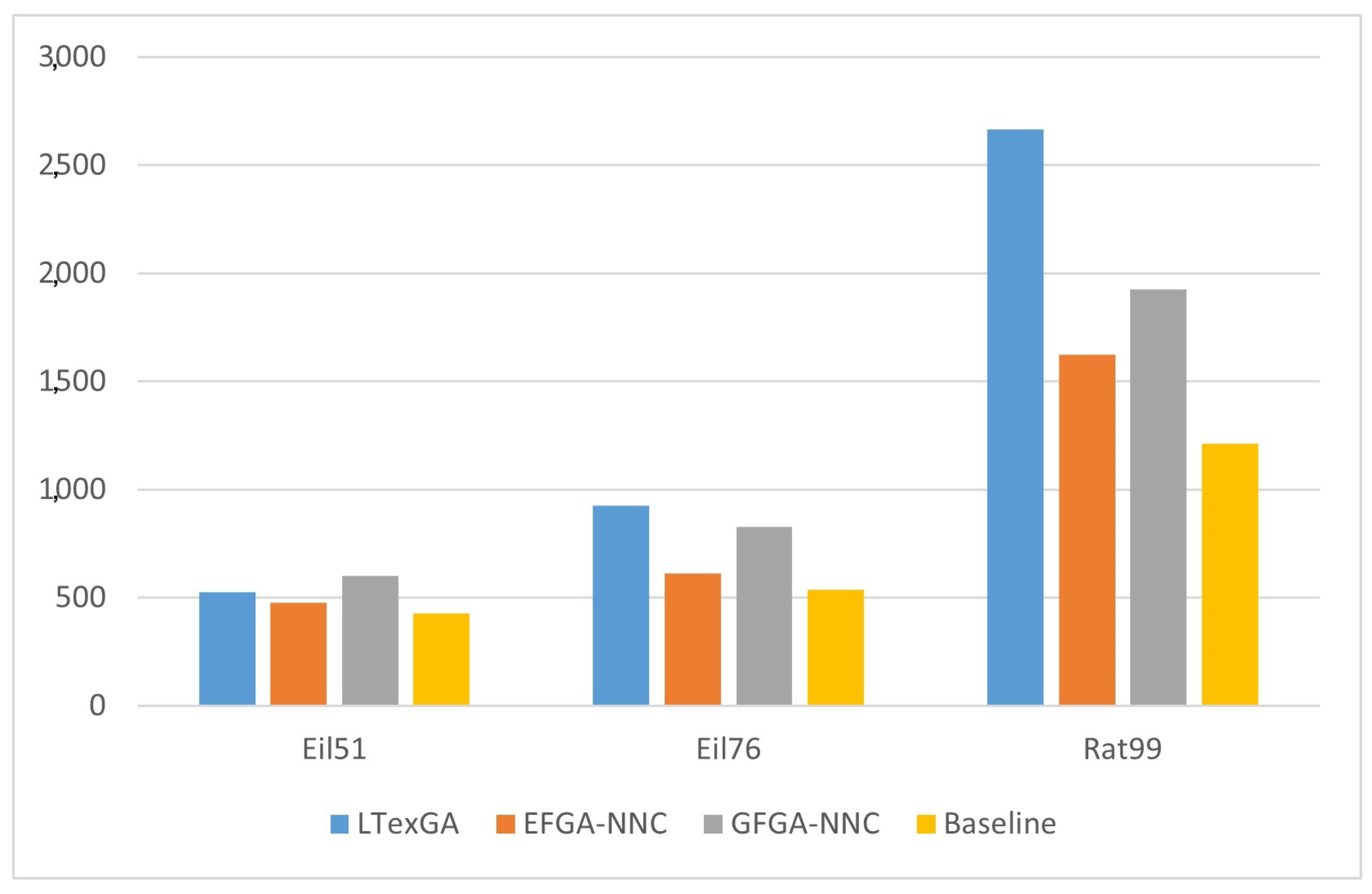
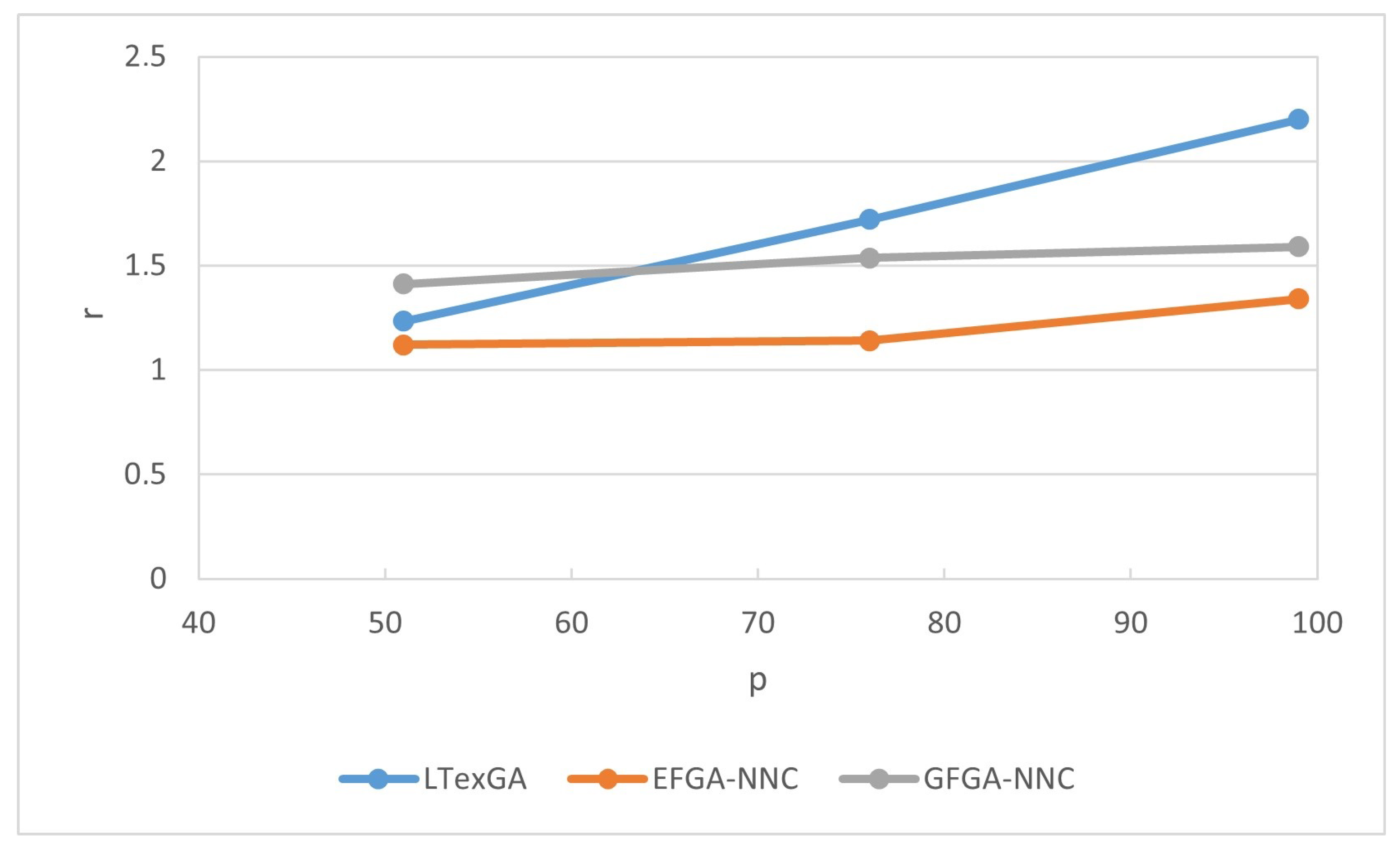
4.3. Traveling Salesman Problem

The traveling salesman problem is another typical benchmark. Given a list of cities and the distances between each pair of cities, the TSP aims to find the shortest possible path such that all cities are visited just once. For a p-city TSP, the distances $x_{ij}$ between the cities $c_i$ and $c_j$ are collected into a $p\times p$ matrix, $\mathbf{X}=\left\{x_{ij}\right\}$, known as the cost matrix. The number of its entries represents the number of variables of the problem, of course. The TSP is an NP-hard problem. Here we refer to [11] for a comparison against published results. Following [11], three problems were taken from TSPLIB95 [25]. They are all symmetric TSPs with Euclidean distance, namely Eil51, Eil76, Rat99, i.e., $p=51$, $p=76$ and $p=99$, respectively. As in [11], we fixed a population size of 100, with 200 generations, through 30 runs. The age linguistic variable in [11] has three terms, i.e., young, middle-aged, and old. In GFGA-NNC, we tried both term sets presented in Section 2.2, even though the first term set with five terms provided the best results. Similarly, for the other term sets, even for EFGA-NNC, increasing from 5 to 7, the number of terms did not produce any significant improvement. For both approaches, the pi-shaped MF was adopted. The best results, i.e., the shortest path length by each approach, are shown in Figure 9. Although neither EFGA-NNC nor GFGA-NNC could outperform the baseline, they represent an improvement with respect to LTexGA [11]. The distance from the baseline grows as the problem cardinality increases. In all cases, EFGA-NNC performed better than GFGA-NNC and LTexGA, keeping the shortest distance from the baseline. EFGA-NNC offers a result very close to the baseline, i.e., 477.34 against 426, especially for Eil51, while it is 525.46 by LTexGA and 601.34 by GFGA.

Figure 8. Average fitness value over the generations for the following: (a) The $g_1$ function; (b) The $g_2$ function.

Figure 8. Average fitness value over the generations for the following: (a) The $g_1$ function; (b) The $g_2$ function.

Let r denote the ratio between the solution obtained by the proposed approaches and the baseline. Figure 10 shows how r varies with p for all the approaches. It can be observed that increasing the problem cardinality does not significantly affect the performance of EFGA-NNC and GFGA-NNC, while LTexGA seems to be influenced by it.

Figure 9. TSP: shortest path length by each approach.

Figure 9. TSP: shortest path length by each approach.

Figure 10. r vs. p.

Figure 10. r vs. p.

4.4. A Real-World Problem: The Case of Rice Production

Rice is a staple crop in Asia, with China and India as the major producers in the world [26]. While rice is not a staple crop in most of Europe, there are countries, such as Italy, that have developed specific traditions around rice cultivation and cuisine. Italy is the main rice producer in Europe [26], with many well-known rice-based recipes. One important stage in the production of rice from paddy (rice with husk) is milling, which is the process of removing the husk and a portion of the bran using techniques like drying, winnowing, and whiting. This process is energy-demanding, requiring proper optimization. Here, we rely on a model discussed in [20], dealing with a case study from Iran, which is solved by GA. The optimization of converting paddy to white rice foresees three goals, i.e., maximize the output energy, minimize the global warming potential (GWP), and maximize the net profit. The GWP contribution represents the cost of CO2 emission. It takes into account climate change damages, and it is one of the most important outputs of the Life Cycle Assessment (LCA) analysis, especially when dealing with crop production and supply chains [27,28,29]. The multi-objective optimization (MOO) problem above can be tackled as a single-objective optimization (SOO) problem (e.g., see [30]). This means that the benefits to be maximized are converted into costs to be minimized. The SOO problem can be tackled by summing up all the single contributions, and the resulting function to be minimized can be written as follows:

$$F(x_1,\dots ,x_6)=\sum _{i=1}^3\sum _{j=1}^6{\alpha }_{ij}{x}_j=\mathbf{A}\mathbf{x},x_j\in X_j,$$

(14)

where $x_1$ is the energy equivalent of human labor, $x_2$ is the energy equivalent of machinery, $x_3$ is the energy equivalent of natural gas, $x_4$ is the energy equivalent of nylon, and $x_5$ is the energy equivalent of transportation. These independent variables can be arranged into a vector $\mathbf{x}$. The respective domains (in MJ ${\mathrm{TIP}}^{-1}$) are the following: $X_1=[44,67]$, $X_2=[92,346]$, $X_3=[675,2005]$, $X_4=[45784,81580]$, $X_5=[934,2240]$, $X_6=[44,133]$. The matrix $\mathbf{A}$ of the coefficients ${\alpha }_{ij}$ is the following:

$$\mathbf{A}=\left(\begin{array}{cccccc}\hfill -0.99& \hfill -2.70& \hfill -1.35& \hfill -2.02& \hfill 0.18& \hfill -0.19\\ \hfill -0.28& \hfill -0.01& \hfill -0.30& \hfill 3.15& \hfill 2.21& \hfill 0.21\\ \hfill -2.64& \hfill -0.44& \hfill -1.58& \hfill 2.85& \hfill 0.42& \hfill 0.65\end{array}\right)$$

(15)

All the numerical values above have been retrieved from [20]. In [20], the best solution was found after 26 generations. No information about the runtime was reported in [20]. The best solutions by EFGA-NNC and GFGA-NNC were retrieved after 43 generations. They are all depicted in Figure 11. The difference between the solutions by EFGA-NNC and the baseline [20] is around 10% on average. Same for GFGA-NNC.

5. Conclusions

In this paper, we focused on two kinds of FGAs, i.e., GFGA and EFGA, which have greatly contributed to the explainability of GAs but present a significant computational burden. To address this issue, we proposed employing a nearest-neighbor caching strategy. We performed several experiments on popular benchmarks, trying different membership functions and logical connectives. Algorithms based on the proposed strategy were compared to the original ones, and different hyperparameters were tried. The results showed significant time savings by means of the proposed NNC strategy, which is the ratio between the runtime with and without NCC ${\displaystyle \frac{9}{200}}$ on average. First, some classical benchmarks were considered, and each FGA type was compared to standard GA and PSO. Except for one case, EFGA with NNC and GA had almost the same performance, while a similar situation was observed for GFGA with NNC for problems with higher dimensions. Secondly, some cases from the literature were considered for a fair comparison against former variants of FGAs. Finally, a real-world application problem was tackled by comparing the results against the ones in the literature. All the results show, in general, the good performance of EFGA with NNC.

The advantage of such a technique is explainability. Even though the NNC allowed for a significant reduction in the runtime, as mentioned before, the standard GA still presents a shorter runtime. This is not surprising since, as discussed in the existing literature, explainability usually brings an additional computational cost. In future work, we plan to investigate how to efficiently deploy the technique for the training of neural networks in order to have an explainable learning process.

References

- Lv, S.; Chen, H. Security Protection Technology in Multi-Attribute Data Transmission Based on Fuzzy Genetic Algorithm. Wirel. Pers. Commun. 2022, 127, 897–917. [Google Scholar] [CrossRef]
- Rajasekar, V.; Predić, B.; Saracevic, M.; Elhoseny, M.; Karabasevic, D.; Stanujkic, D.; Jayapaul, P. Enhanced multimodal biometric recognition approach for smart cities based on an optimized fuzzy genetic algorithm. Sci. Rep. 2022, 12, 622. [Google Scholar] [CrossRef] [PubMed]
- Ashtari, P.; Karami, R.; Farahmand-Tabar, S. Optimum geometrical pattern and design of real-size diagrid structures using accelerated fuzzy-genetic algorithm with bilinear membership function. Appl. Soft Comput. 2021, 110, 107646. [Google Scholar] [CrossRef]
- Jahan, A.; Mollazadeh, M.; Akbarpour, A.; Khatibinia, M. Health monitoring of pressurized pipelines by finite element method using meta-heuristic algorithms along with error sensitivity assessment. Struct. Eng. Mech. 2023, 87, 211–219. [Google Scholar]
- Song, P.; Chen, C.; Zhang, L. Evaluation Model of Click Rate of Electronic Commerce Advertising Based on Fuzzy Genetic Algorithm. Mob. Netw. Appl. 2022, 27, 936–945. [Google Scholar] [CrossRef]
- Wang, S.; Hui, J.; Zhu, B.; Liu, Y. Adaptive Genetic Algorithm Based on Fuzzy Reasoning for the Multilevel Capacitated Lot-Sizing Problem with Energy Consumption in Synchronizer Production. Sustainability 2022, 14, 5072. [Google Scholar] [CrossRef]
- Song, Y.H.; Wang, G.S.; Wang, P.Y.; Johns, A.T. Environmental/economic dispatch using fuzzy logic controlled genetic algorithms. Gener. Transm. Distrib. 1997, 144, 377. [Google Scholar] [CrossRef]
- Subbu, R.; Sanderson, A.C.; Bonissone, P.P. Fuzzy logic controlled genetic algorithms versus tuned genetic algorithms: An agile manufacturing application. In Proceedings of the 1998 IEEE International Symposium on Intelligent Control (ISIC) Held Jointly with IEEE International Symposium on Computational Intelligence in Robotics and Automation (CIRA), Piscataway, NJ, USA, 17 September 1998; pp. 434–440. [Google Scholar]
- Wang, K. A new fuzzy genetic algorithm based on population diversity. In Proceedings of the 2001 IEEE International Symposium on Computational Intelligence in Robotics and Automation (Cat. No.01EX515), Banff, AB, Canada, 29 July–1 August 2001; pp. 108–112. [Google Scholar]
- Yun, Y.; Gen, M. Performance analysis of adaptive genetic algorithms with fuzzy logic and heuristics. Fuzzy Optim. Decis. Mak. 2003, 2, 161–175. [Google Scholar] [CrossRef]
- Last, M.; Eyal, S. A fuzzy-based lifetime extension of genetic algorithms. Fuzzy Sets Syst. 2005, 149, 131–147. [Google Scholar] [CrossRef]
- Liu, H.; Xu, Z.; Abraham, A. Hybrid fuzzy-genetic algorithm approach for crew grouping. In Proceedings of the 5th International Conference on Intelligent Systems Design and Applications (ISDA05), Wroclaw, Poland, 8–10 September 2005; pp. 332–337. [Google Scholar]
- Li, Q.; Tong, X.; Xie, S.; Liu, G. An improved adaptive algorithm for controlling the probabilities of crossover and mutation based on a fuzzy control strategy. In Proceedings of the 2006 Sixth International Conference on Hybrid Intelligent Systems (HIS06), Rio de Janeiro, Brazil, 13–15 December 2006; pp. 50–56. [Google Scholar]
- Jafari, S.A.; Mashohor, S.; Varnamkhasti, M.J. Committee neural networks with fuzzy genetic algorithm. J. Pet. Sci. Eng. 2011, 76, 217–223. [Google Scholar] [CrossRef]
- Venkatanareshbabu, K.; Nisheel, S.; Sakthivel, R.; Muralitharan, K. Novel elegant fuzzy genetic algorithms in classification problems. Soft Comput. 2018, 23, 5583–5603. [Google Scholar] [CrossRef]
- Singh, M.; Brownlee, A.E.I.; Cairns, D. Towards Explainable Metaheuristic: Mining Surrogate Fitness Models for Importance of Variables. In Proceedings of the GECCO22, Boston, MA, USA, 9–13 July 2022; pp. 1785–1793. [Google Scholar]
- Pandey, S.; Broder, A.; Chierichetti, F.; Josifovski, V.; Kumar, R.; Vassilvitskii, S. Nearest-Neighbor Caching for Content-Match Applications. In Proceedings of the International World Wide Web Conference (WWW 2009-ACM), Madrid, Spain, 20–24 April 2009; pp. 441–451. [Google Scholar]
- Niesen, U.; Shah, D.; Wornell, G.W. Caching in Wireless Networks. IEEE Trans. Inf. Theory 2012, 58, 6524–6540. [Google Scholar] [CrossRef]
- Bagheri, E.; Deldari, H. Dejong Function Optimization by means of a Parallel Approach to Fuzzified Genetic Algorithm. In Proceedings of the 11th IEEE Symposium on Computers and Communications (ISCC’06), Cagliari, Italy, 26–29 June 2006; pp. 675–680. [Google Scholar]
- Nabavi-Pelesaraei, A.; Rafiee, S.; Mohtasebi, S.S.; Hosseinzadeh-Bandbafha, H.; Chau, K.W. Assessment of optimized pattern in milling factories of rice production based on energy, environmental and economic objectives. Energy 2019, 169, e1259–e1273. [Google Scholar] [CrossRef]
- Chierichetti, F.; Kumar, R.; Vassilvitskii, S. Similarity Caching. In Proceedings of the 28th ACM SIGMOD-SIGACT-SIGART Symposium on Principles of Database Systems (PODS-09), San Diego, CA, USA, 9–12 June 2009; pp. 127–135. [Google Scholar]
- Li, Q.; Yin, Y.; Wang, Z.; Liu, G. Comparative Studies of Fuzzy Genetic Algorithms. In Proceedings of the Advances in Neural Networks—ISNN 2007: 4th International Symposium on Neural Networks, ISNN 2007, Nanjing, China, 3–7 June 2007. [Google Scholar]
- Li, Q.; Zheng, D.; Tang, Y.; Chen, Z. A New Kind of Fuzzy Genetic Algorithm. J. Univ. Sci. Technol. 2001, 1, 85–89. [Google Scholar]
- Kuang, T.; Hu, Z.; Xu, M. A Genetic Optimization Algorithm Based on Adaptive Dimensionality Reduction. Available online: https://onlinelibrary.wiley.com/doi/10.1155/2020/8598543 (accessed on 5 November 2024).
- Available online: http://comopt.ifi.uni-heidelberg.de/software/TSPLIB95/ (accessed on 5 November 2024).
- Faostat-Crops and Livestock Products. Available online: www.fao.org/faostat/en/#data/QCL (accessed on 5 November 2024).
- Tomasiello, S.; Uzair, M.; Liu, Y.; Loit, E. Data-driven approaches for sustainable agri-food: Coping with sustainability and interpretability. J. Ambient. Intell. Humaniz. Comput. 2023, 14, 16867–16878. [Google Scholar] [CrossRef]
- D’Arienzo, M.P.; Raritá, L. Management of Supply Chains for the Wine Production. In Proceedings of the International Conference on Numerical Analysis and Applied Mathematics 2019, ICNAAM 2019, Rhodes, Greece, 23–28 September 2019. [Google Scholar]
- Raritá, L. A Genetic Algorithm to Optimize Dynamics of Supply Chains; AIRO Springer Series; Springer: Berlin/Heidelberg, Germany, 2022; Volume 8, pp. 107–115. [Google Scholar]
- Naderi, R.; Nikabadi, M.S.; Tabriz, A.A.; Pishvaee, M.S. Supply chain sustainability improvement using exergy analysis. Comput. Ind. Eng. 2021, 154, 107142. [Google Scholar] [CrossRef]
Disclaimer/Publisher’s Note: The statements, opinions and data contained in all publications are solely those of the individual author(s) and contributor(s) and not of MDPI and/or the editor(s). MDPI and/or the editor(s) disclaim responsibility for any injury to people or property resulting from any ideas, methods, instructions or products referred to in the content. |
© 2024 by the authors. Licensee MDPI, Basel, Switzerland. This article is an open access article distributed under the terms and conditions of the Creative Commons Attribution (CC BY) license (https://creativecommons.org/licenses/by/4.0/).
Share and Cite
Syzonov, O.; Tomasiello, S.; Capuano, N. New Insights into Fuzzy Genetic Algorithms for Optimization Problems. Algorithms 2024, 17, 549. https://doi.org/10.3390/a17120549
Syzonov O, Tomasiello S, Capuano N. New Insights into Fuzzy Genetic Algorithms for Optimization Problems. Algorithms. 2024; 17(12):549. https://doi.org/10.3390/a17120549
Chicago/Turabian StyleSyzonov, Oleksandr, Stefania Tomasiello, and Nicola Capuano. 2024. "New Insights into Fuzzy Genetic Algorithms for Optimization Problems" Algorithms 17, no. 12: 549. https://doi.org/10.3390/a17120549
APA StyleSyzonov, O., Tomasiello, S., & Capuano, N. (2024). New Insights into Fuzzy Genetic Algorithms for Optimization Problems. Algorithms, 17(12), 549. https://doi.org/10.3390/a17120549