
Comparing Direct Deliveries and Automated Parcel Locker Systems with Respect to Overall CO2 Emissions for the Last Mile


1
Institute of Information Engineering, Ostfalia University of Applied Sciences, 38302 Wolfenbüttel, Germany
2
IT in Production and Logistics, Faculty of Mechanical Engineering, TU Dortmund, 44227 Dortmund, Germany
3
Center for International Migration (GIZ/CIM), 65760 Eschborn, Germany
4
Logistics Living Lab—Ecuador (L3E), Quito 170135, Ecuador
*
Author to whom correspondence should be addressed.
Algorithms 2024, 17(1), 4; https://doi.org/10.3390/a17010004
Submission received: 1 November 2023
/
Revised: 10 December 2023
/
Accepted: 15 December 2023
/
Published: 21 December 2023
(This article belongs to the Special Issue Optimization Algorithms in Logistics, Transportation, and SCM)
Abstract
:Fast growing e-commerce has a significant impact both on CEP providers and public entities. While service providers have the first priority on factors such as costs and reliable service, both are increasingly focused on environmental effects, in the interest of company image and the inhabitants’ health and comfort. Significant additional factors are traffic density, pollution, and noise. While in the past direct delivery with distribution trucks from regional depots to the customers might have been justified, this is no longer valid when taking the big and growing numbers into account. Several options are followed in the literature, especially variants that introduce an additional break in the distribution chain, like local mini-hubs, mobile distribution points, or Automated Parcel Lockers (APLs). The first two options imply a “very last mile” stage, e.g., by small electrical vehicles or cargo bikes, and APLs rely on the customers to operate the very last step. The usage of this schema will significantly depend on the density of the APLs and, thus, on the density of the population within quite small regions. The relationships between the different elements of these technologies and the potential customers are studied with respect to their impact on the above-mentioned factors. A variety of scenarios is investigated, covering different options for customer behaviors. As an additional important point, reported studies with APLs only consider the section up to the APLs and the implied CO2 emission. This, however, fully neglects the potentially very relevant pollution created by the customers when fetching their parcels from the APL. Therefore, in this paper this impact is systematically estimated via a simulation-based sensitivity analysis. It can be shown that taking this very last transport step into account in the calculation significantly changes the picture, especially within areas in outer city districts.
1. Introduction
E-commerce is experiencing significant growth in various countries and sectors. This increase in online sales presents never before seen unique logistical challenges for businesses, one of the most critical being the efficient management of the last mile—the final stage of the delivery process that ends at the customer’s home or at a designated pickup point [1]. Last-mile logistics (LML) plays a critical role in influencing service levels [2] and contributes significantly to overall logistics costs [3].
In the search for innovative solutions to address these challenges, automated parcel lockers (APLs) have emerged as a compelling option. APLs are boxes with automated locks, clustered in structures. APLs are often found in public areas such as supermarkets or train stations and serve multiple customers [4]. APLs are a promising alternative to traditional direct delivery (DD) for several reasons: their ease of access to customers [2], their ability to handle higher delivery densities [5], and their significant reduction in the likelihood of delivery failures [6]. Consequently, researchers and practitioners are both exploring the potential benefits of APLs in the e-commerce delivery. Managers also have shown great interest in understanding the economic impact of APLs compared to DD [7,8].
The current literature primarily emphasizes delivery cost benefits, but there is still a scarcity of papers addressing vehicle kilometers traveled (VKT), emissions, and customer trips for parcel pick-ups.
This work develops a simulation model that allows for a comparison between DD and APLs as an LML scheme. Various factors are analyzed that distinguish between these contexts, such as CO2 emissions and VKT, to gain a comprehensive understanding of their implications, as well as taking additional transports for customers to pick up their parcels at the APLs into account. In this context, the approach presented in this paper includes a more detailed model to estimate the emissions of customers to reach APLs.
Moreover, previous work comparing delivery through APLs and DD is based on an estimated demand of the delivery process that does not accurately reflect real-world scenarios. This paper introduces a more realistic configuration. It investigates the case of the city of Dortmund, which is located in the federal state North Rhine-Westphalia, Germany. With a population of about 600,000 people, it is the seventh largest city in Germany and the 34th largest city in the European Union. By addressing the described weaknesses and taking a more comprehensive and realistic approach, the research aims to provide valuable insights into the reductions of CO2 emission by using DD and APLs for different delivery contexts and offering more-accurate and applicable conclusions. Addressing all the identified issues will lead to a comprehensive and clear understanding of the advantages that APLs offer over traditional DD. This goal is addressed through the following research questions (RQs):
- RQ1. What is the average CO2 emission through APLs compared to traditional DD?
- RQ2. How does this comparison change under different demand scenarios and different assumptions regarding customer behavior for picking up parcels?
To address these questions, the study uses a simulation approach that includes two distinct stages. In the first stage, a comprehensive model has been developed to estimate CO2 emissions for both APLs and DD. In the second stage, a simulation model was applied to provide more-accurate numerical insights to effectively answer the RQs. This simulation-based methodology ensures a thorough analysis of the environmental impact of APL and DD and provides valuable information for informed decision-making.
The structure of this paper is as follows: First, the results of the literature review are presented. The simulation model and its application are illustrated in the following two sections. Finally, we summarize the conclusions of our work.
2. Related Work
In their comprehensive review of innovative LML solutions, the authors in [7] highlight the importance of investigating the potential savings associated with APLs compared to traditional DD. This research is critical for making informed management decisions and encouraging the adoption of APLs in logistics operations. In addition, a study by [9] highlights the lack of scientific literature on APLs when it comes to the LML. This suggests that further research and analysis is needed in this area to fully understand and exploit the benefits of APLs as an alternative to DD.
The main research on APLs can be divided into two groups. The first, which is more extensive, is devoted to the problem of operating distribution networks. This involves finding optimal routes to efficiently serve customers within a given area, i.e., solving the associated vehicle routing problems (VRPs). The second group focuses on determining the optimal number and geographical locations of APLs, i.e., solving associated strategic facility location problems (FLPs) for implementing APLs as a viable alternative to DD. This line of research aims to investigate how APLs can effectively improve the last-mile delivery process by providing potential solutions to the challenges faced by traditional delivery systems.
2.1. Vehicle Routing Problems
Given a set of transport orders and a fleet of vehicles with given capacities, the VRP aims to minimize the total traveled distance; the number of tours; or—more generally—the travel costs for fulfilling all transport orders meeting all given constraints, which due to capacity constraints typically relate to the volume or weight of the given transport items. For private entities, minimizing traveled distances is critical because it directly affects load factors and costs. On the other hand, for the public actors reducing the traveled distance is paramount as it directly affects pollution and city traffic.
The VRP was first introduced by [10] in the late 1950s. They formulated the mathematical programming approach and algorithm to solve the problem of delivering gasoline to gas stations. Over the years, the VRP has proven to be a valuable tool for optimizing transport operations. Minimizing the total traveled distance or optimizing the number of vehicles required can significantly improve transport costs.
Descriptions of VRP methods can be found in lecture books on logistics. A comprehensive explanation of several algorithms and their function, including the enrichment towards the team orientation problem (TOP), can be found, e.g., in [11].
In this context, ref. [12] provided a comprehensive and extended overview of the VRPs for LML and its diverse applications, with a particular focus on incorporating the perspectives of local authorities and companies. Additionally, several operational tools were introduced by [13,14,15,16]. These studies offer valuable insights into practical solutions and strategies to address the challenges posed by LML, thus enhancing the efficiency and sustainability of transport operations in urban areas.
In the realm of alternative delivery locations, several notable studies have contributed to the field. In [17], the authors presented an early work that addresses the vehicle routing problem with roaming delivery locations. In their model, customers receive deliveries in different non-overlapping time windows at different delivery points, e.g., by getting packages delivered to their parked car throughout the day. The authors highlight the advantages of roaming delivery over traditional home delivery and emphasize its cost-effectiveness.
Ref. [18] looked at a different facet of alternative delivery, considering direct-to-customer delivery or delivery through pickup points. They framed this as a multi-depot two-echelon vehicle routing problem. While their study examined various delivery options, it did not consider capacity constraints at pickup points. In this regard, ref. [19] studied a distribution system with capacitated locker stations and ignored home deliveries and customer time windows. However, they considered different sizes for the APLs. Nevertheless, the restriction to only one parcel per slot simplified the packing decisions. The work of [20] addressed the inclusion of capacity constraints at alternative delivery locations. However, they did not include time windows for customers at their home locations in the problem.
In addition, ref. [21] addressed the vehicle routing problem with private and shared delivery locations, which is closely related to our problem. Their private locations represented home delivery points, while the shared locations were APLs stations. However, they did not consider the different parcel and slot sizes. Their approach uses a matheuristic based on finding large neighborhoods, with a repair step using a mixed integer programming model and integrated iterated local search to avoid getting stuck in local optima. A study by [22] explored the concept of mobile APLs with dynamically changing locations. They focused on optimally locating these mobile APLs so that customers stay within a certain range of their assigned station during the planning horizon. The goal was to minimize the locker fleet.
Ref. [23] proposed a VRP with soft time windows for last-mile delivery and studied the impact of the introduction of lockers. The problem aims at minimizing the variable transport costs, the soft time windows penalty, the CO2 emission costs, and the fixed costs of labor and vehicles. Once the lockers are introduced, the time window constraints are not considered anymore, but the locker renting costs and the new small vans’ acquisition costs are included in the objective function.
2.2. Facility Location Problems
Facility location is an important and fundamental strategic decision that strongly influences tactical and operational aspects in any organization. Such location decisions are common at various levels of human organizations, from individuals and households to corporations, government agencies, and international organizations. The study of location decisions has a long tradition in the literature. The FLP emerged in the 1960s in the field of operations research [24] and was initially called the plant location problem.
The FLPs represent classical optimization problems that involve finding optimal locations for facilities. These problems involve determining the most appropriate locations for one or many facilities to efficiently serve a set of demand points. The definition of the “best” location varies depending on the nature of the specific problem, taking into account constraints and optimality criteria [25]. FLPs have applications in a wide variety of settings where strategic placement is required, including hospitals, fire stations, bus stops, train stations, truck terminals, gas stations, blood bank centers, retail stores, libraries, parks, post offices, airports, and landfills.
There are sufficient detailed descriptions of FLP algorithms in the literature. A concise but detailed explanation, with an additional investigation of uncertainty and a focus on FLP for supply chains, is provided by [26].
The versatility of FLPs makes them a mandatory tool for optimizing the location of critical facilities and services in a variety of real-world scenarios. Various applications of FLPs can be found in the context of LML [27,28,29,30,31,32,33,34]. Farahani et al. [35] have provided a comprehensive overview of the applications of FLPs and explored future developments in this field. In [5], the authors presented a remarkable application of FLP in APLs for static situations. However, the dynamic aspects of the problem were largely ignored, such as variability in customer willingness to use the service and operational setup costs.
Ref. [36] explored healthcare logistics and devised a solution that combines a facility location problem with routing to efficiently supply medications to patients, while minimizing delivery costs. Their study focused on serving patients within the service area of APLs, leaving the remaining demand to be fulfilled through home delivery. Another study by [37] explored using existing infrastructure like supermarkets and gas stations as potential APL locations. While they determined optimal locations based on customer density, they overlooked important factors such as costs and environmental aspects. In [38], the study focused on maximizing profit by determining suitable APL locations. They used a threshold Luce model to represent discrete customer choice, where APL users choose the closest facility or select from a set of APLs. However, they overlooked shipping costs in their analysis, which is a crucial aspect of efficient network design.
A dynamic approach was taken by [22]. They optimized the locations of mobile parcel lockers that can adapt to recipients’ whereabouts during different time periods. Despite their valuable contributions, these studies failed to consider a holistic LML network encompassing both home and APL deliveries, which is essential for accurately representing the perspective of a logistics service provider. Moreover, an important aspect overlooked in previous research was the external impact, specifically CO2 emissions generated during the delivery process and APL usage. In recent times, e-commerce retailers have been reshaping their strategies to minimize CO2 emissions, making it crucial to incorporate environmental considerations when designing APL networks. For example, the e-commerce retailer Zalando has already achieved carbon-neutral in-house operations and carbon-neutral shipping and return processes [39].
The authors of [40] investigate APLs in two areas (rural and suburban) in an experimental set-up. In their simulation, they measure the overall CO2 emissions from deliveries and pickups and find a positive effect in most instances, with up to 40% CO2 savings using APLs. The authors of [41] evaluate the impact of APLs on reducing several pollutants. They study the effect in New York City and use bike-sharing stations as potential APL locations. Furthermore, they offer a comprehensive overview of research on emissions involving APLs. Even though all of these studies consider emissions, e.g., [42,43,44,45,46,47], only some include customer pickups explicitly [48,49,50,51].
The results presented by [47] indicate the substantial benefits from implementing APLs for both the operator and the municipality. The overall VKT were cut by 90.9%, rendering nearly 80% of the vehicle fleet unnecessary. The model architecture comprises three key components: (i) customer location, specifying whether the customer’s house is in an urban or extra-urban area; (ii) average distance needed to reach the APLs for customers; and (iii) average distance between two APLs (density of APLs). The authors incorporated emission factors within DD and APLs based on interviews with major logistics operators in Italy. The model does not include detailed locations of customers and APLs or algorithms to solve VRP instances.
Ref. [48] suggests that the environmental benefits of an APL remain valid for the community, including couriers and customers, as long as the distance a customer must travel by car to reach the APL is within 0.94 km in urban areas and 6 km in rural areas. On the selected simulation day, five vehicles executed 70 delivery stops for DD in a given area from 11:00 a.m. to 4:30 p.m. For a comparison with an APL network for the same area, the estimation focused on the number of cars involved in collecting parcels from the APLs. The simulation considered only the car option among various modes of transport to and from the APLs, i.e., pedestrian movements, cycling, and public transport were not an integral part of the model.
Refs. [49,50]’s findings accurately represent the daily operations of a carrier serving West Sussex, extrapolating over a year with 62,400 deliveries. The authors look at a different process, where customers only pick up parcels at so called collection-and-delivery points (CDPs), in case that they were not at home when visited by a vehicle of the carrier on a DD tour. The most significant savings in emissions, with a 44% reduction, occurred when local post offices were utilized as CDPs. This outcome was based on the assumption that 50% of the deliveries failed initially, and 30% of those unsuccessful deliveries resulted in consumers collecting their packages from the carrier’s depot (87% by car). Emissions from both the carrier and household were quantified for different CDP configurations and compared to DD visiting customers a second or even a third or fourth time. The results showed that CDP delivery systems led to a reduction in emissions ranging from 48% to 58% compared to the traditional approach of only DD.
The findings outlined in [51] conducted an evaluation of the freight component in failed deliveries. It was observed that the additional CO2 emitted during the second delivery attempt resulted in an increase in emissions per drop, ranging from 9% to 75%. The predominant emissions (85% to 95%) from a failed DD result not from the subsequent van re-delivery but from the individual customer traveling to collect a missed delivery from the carrier’s local depot. Various CDPs (supermarkets, post offices, and railway stations) were identified as effective at reducing the environmental impact of this personal travel. Notably, post offices yielded the most significant savings in this context, accounting for only 13% of the CO2 produced in comparison to a collection by car directly from a local depot. Again, the presented research focuses solely on potential CO2 savings for failed deliveries.
In their study, the authors of [52] employed a multinomial logistic model to assess the inclination of customers to utilize APLs, taking into consideration factors such as APL availability at home and travel distance. Their analysis of various regional clusters revealed that strategically locating APLs could yield cost savings of up to 11.0%. While APLs demonstrated a positive impact on overall CO2 emission reduction in urban areas (up to 2.5%), they concurrently led to additional emissions (4.6%) in less populated regions due to extended travel distances during the pickup process.
Building upon this, ref. [53] presented a location and routing problem formulation for last-mile delivery services employing APLs. They introduced a mathematical model based on mixed integer programming to optimize the environmental impact by minimizing distances traveled by both the delivery company and consumers. The model incorporated consumer behavior through two parameters: the maximum acceptable travel distance to reach an APL using any means of transport and the maximum eco-friendly distance a consumer is willing to travel by foot or bicycle, thus producing no CO2 emissions.
Furthermore, ref. [54] conducted an analysis of the CO2 impact associated with APLs in last mile parcel delivery. Employing continuous approximation techniques, the paper assessed the potential enhancement in delivery route efficiency. Multinomial logistic regression was utilized to estimate travel distance and mode choice for customers collecting their parcels. The study underscored the importance of weighing the efficiency gains for the delivery vehicle against the environmental impact of customers traveling to the APL, particularly when using private cars.
In summary, the research in the field has laid a solid foundation for the current study. The extensive investigation of various aspects of alternative APL locations, including roaming delivery, pickup points, lockers with capacity, and home and shared delivery locations, has delivered valuable insights. Building upon these findings, the primary objective is to tackle the challenges related to CO2 emissions while simultaneously optimizing the routing process. The comprehensive analysis of alternative APL locations has provided a basis for further exploration and refinement. With a focus on sustainability, the aim is to derive innovative strategies to reduce CO2 during the delivery process. By implementing environmentally friendly practices and leveraging state-of-the-art routing technologies, the overall efficiency of APL systems should be enhanced. Therefore, this research is contributing significantly to the field of LML and sustainable transport.
The final research goal is to develop a practical and environmentally conscious solution that not only benefits businesses and consumers but also contributes positively to the environment. By addressing the critical issues associated with CO2 emissions in the delivery sector, the way could be paved for a greener and more sustainable future.
3. System Configurations
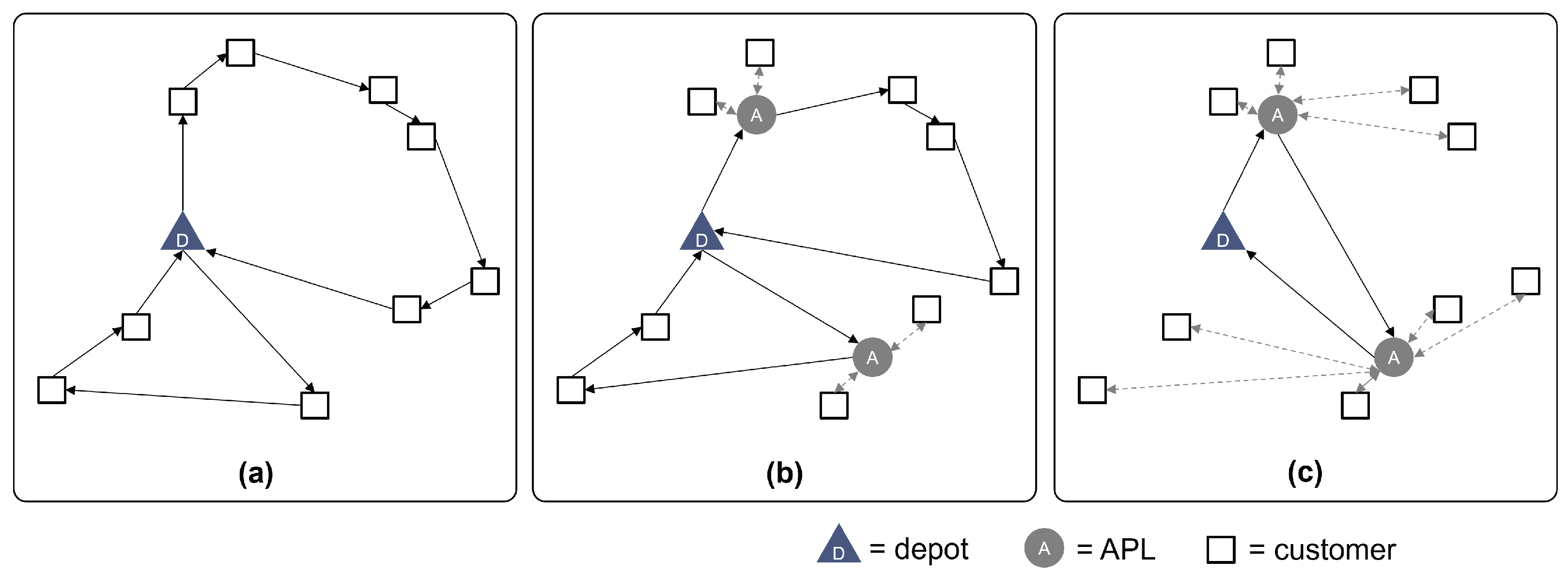
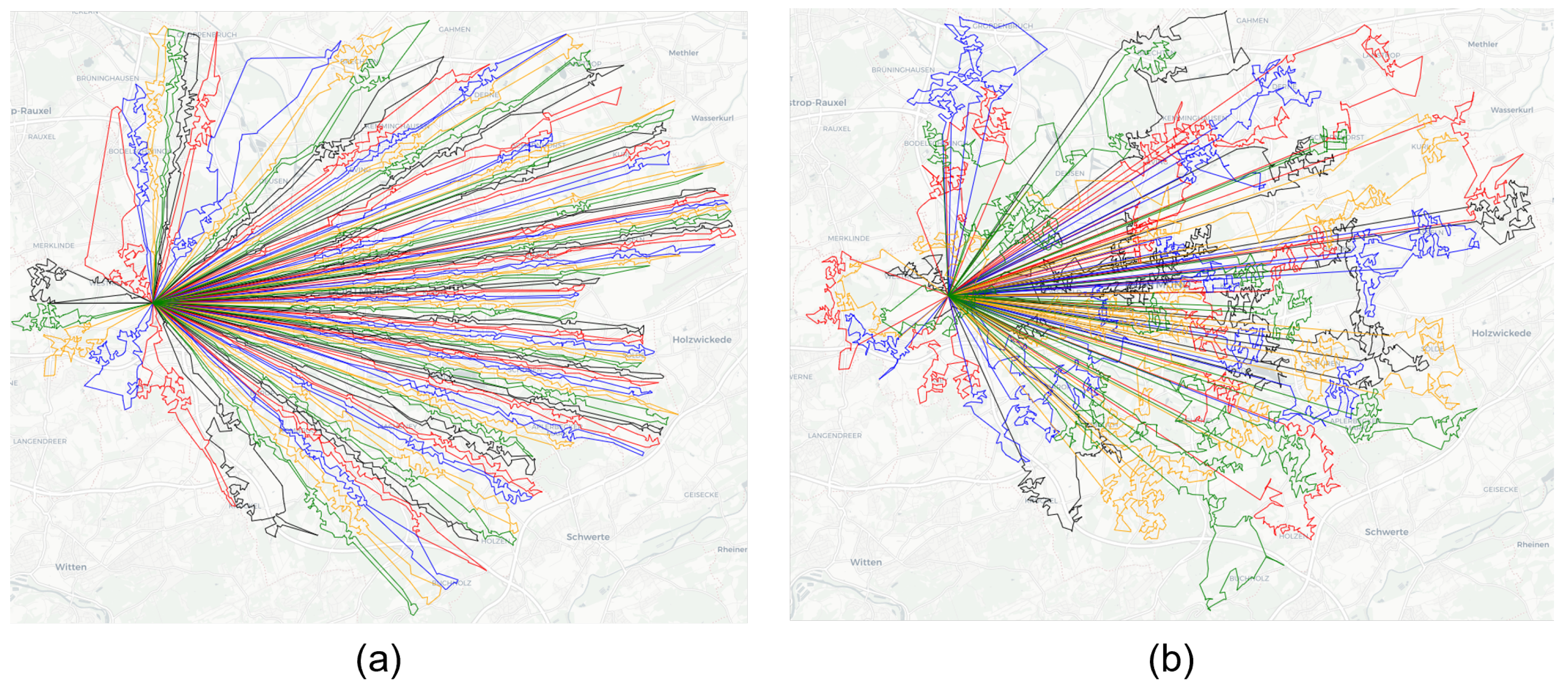
For determining valid delivery plans for the last mile, typical instances of the VRP need to be solved, especially if vehicles with limited capacity are considered. Different system configurations are investigated with only one central depot or several depots, from where all tours to the final customers start and end (Figure 1a). Furthermore, hubs can be introduced to the distribution system with central depots serving all hubs, from where the customers are served. In this case, VRP problems may also occur for serving the hubs from the depot.
A customer within such a system could also be represented as an APL, where parcels are buffered to be picked up by the final recipients. Figure 1b) reflects such an approach, where the service provider plans routes to multiple recipients, including APLs. In extreme cases, all recipients choose to utilize APLs (Figure 1c).
The key question is which approach is more efficient in terms of distance traveled and CO2 emissions. A comparison of the different approaches can provide insight into the respective advantages and disadvantages in optimizing delivery operations.
4. Modeling Approaches to Assess the Costs for the Last Mile for Direct Deliveries
This research is focused on systems with one central depot, from where customers (or APLs) are served by a fleet of vehicles. Three different approaches (at different aggregation levels) are discussed in the following sub-sections and compared to direct deliveries. The capacity of each vehicle is restricted by a given number of parcels, which serves as a rough abstraction of actually relevant weight or volume restrictions. Solving the underlying VRP consists of two different problems:
- Defining clusters of customers (to be served on a single tour),
- Defining the sequence in which the customers are served on the tours.
Using mathematical optimization, these two problems are solved simultaneously. However, as the VRP is an np-hard problem, only relatively small problem instances can be solved to optimality within a reasonable amount of time. Therefore, usually heuristic approaches are applied. Here, construction and improvement methods are further distinguished [55].
The nearest neighbor construction method starts with a single node (from the set of all nodes to be visited) as the current node i (usually the depot). The nearest node (from the set of nodes not visited yet) to the current node i is chosen to be visited next and set as the current node for the next iteration. Once all of the nodes have been visited, the tour is closed by returning to the first node (depot).
Often, two well-known heuristic approaches, the sweep and the savings algorithm, are applied to solve VRP instances and have also been implemented in this paper. Originally introduced in the seminal work [56], the sweep algorithm operates as follows: starting from the depot location as the origin, a sweeping line is extended outward in a predetermined direction. As this line sweeps around the depot, it groups nodes within its vicinity for a single tour until the capacity constraints are reached. Once the members of a tour have been determined, the respective instance of the TSP is solved.
The savings algorithm is a construction heuristic that seeks to minimize the total distance traveled by vehicles while serving a set of customers [57]. The algorithm starts with the worst-case solution that each customer is served on a single tour. It calculates possible savings for each pair of tours (customers), representing the potential reduction in distance if the two tours are combined in a single tour. These savings are sorted, and the procedure iteratively merges tours (if within the the capacity constraints), gradually forming the final solution. The savings algorithm shows simplicity as well as effectiveness in generating reasonable solutions [55]. While it might not always produce optimal solutions, its efficiency and adaptability make it a valuable tool in practice.
Moreover, such construction algorithms can be enhanced by integrating additional heuristics or local search techniques to refine the initial solution, achieving improved results in practice. A typical example for an improvement procedure is 2-Opt, where in each iteration two edges are eliminated from the existing tour. The two remaining parts of the original tour are reconnected after changing the direction of visiting the nodes of one of the two parts, following a greedy approach resulting in a shorter tour.
For the purpose of the model described in this paper, it might not be necessary to implement these methods in detail and to simulate the daily planning of tours, which eventually leads to relatively long computational times. Instead, (simple) formulas from the literature could also be applied for estimating the distance traveled for a given number of transport orders. In conclusion, there are different levels of abstraction that are used for estimating the costs for last-mile deliveries in this paper:
- estimation of the kilometers driven by a simple formula.
- estimation of the kilometers driven for (given) districts by solving instances of the TSP for each district.
- estimation of the kilometers driven by solving the overall VRP problem in one step (on the basis of the sweep or savings algorithm).
These approaches are discussed in detail in the following sub-sections. Results comparing these approaches are given in Section 6.
4.1. Estimation of the Kilometers Driven for Each Tour (Round Trip)
The input variables for estimating the distance d driven for each tour are the size of the area A (Figure 2a) and the number of customers n to be visited (Equation (1)) [58,59]:
Given the need to plan multiple round trips, the total area needs to be divided according to the expected number of tours. Given the daily number of parcels and the number of parcels per tour (the capacity of the vehicle), the area served within each tour could be estimated by dividing the total area of the city by the total number of expected tours. However, the assumption that the transport orders are evenly distributed over the city area is not realistic. Typically, the number of orders correlates with the size of the population.
In this context, all of the necessary data are given for city districts for the example of the city of Dortmund. From the associated data, the number of tours per district is calculated. A possible estimation of the total distance traveled could be to simply divide the area of the district by the number of necessary tours per district. Then, Equation (1) could be applied to compute the average tour length, adding the distance from the depot to the district and back for each tour. However, following this strategy leads to tours that are usually not fully utilized. An alternative is to assume fully utilized tours. For each district A, the remaining parcels for a last, not fully utilized tour are transferred to the next (neighbor) district B to be planned, increasing the tour of the neighbor district B by the respective ratio of left orders in relation to the total number of orders of district A.
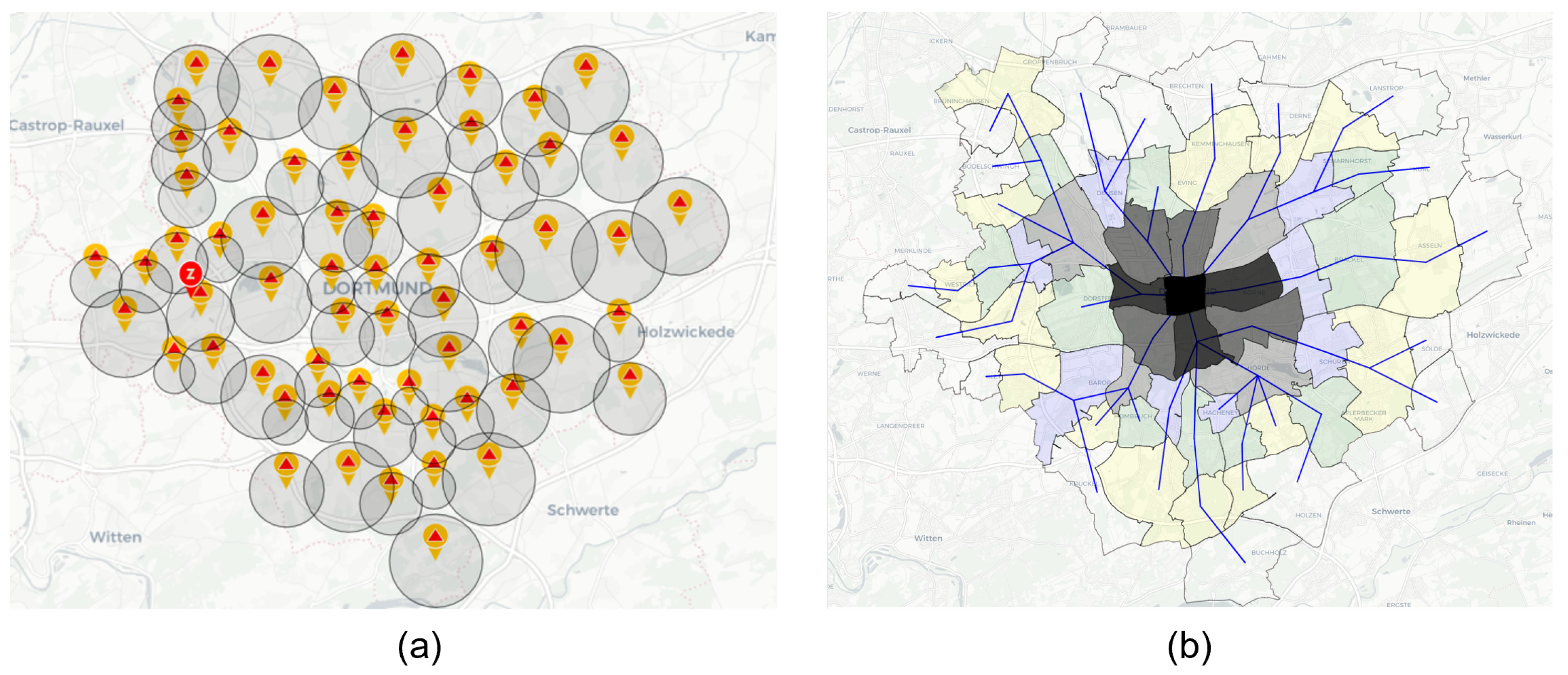
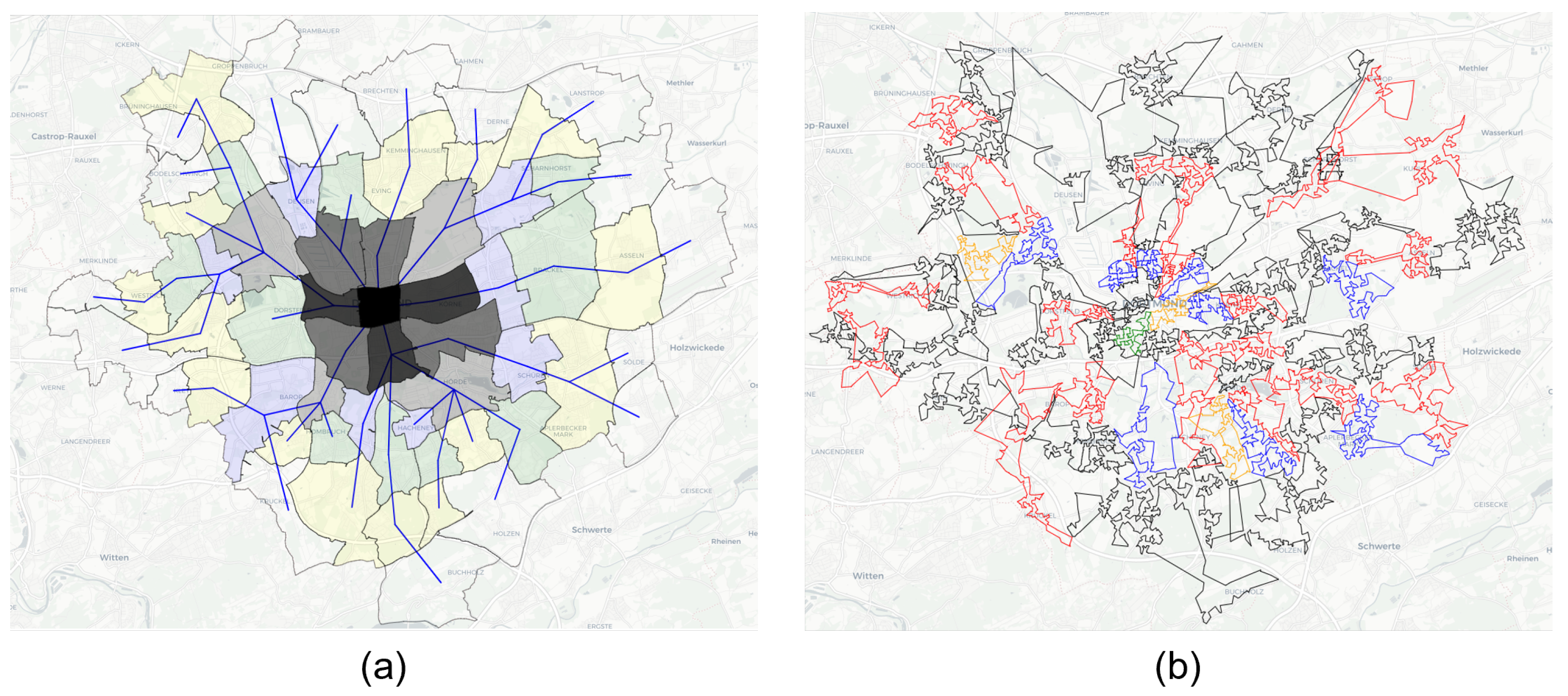
More formally, the approach can be formulated as follows: The maximum capacity of the vehicle is C, and the number of full-truck loads is , with for district j. The area to be visited by full truck tours is given by . For each tour, an area of for C parcels is assumed. If parcels remain, these are transferred to a (previously defined) neighbor district that has not been planned yet. Additionally, the remaining area () is added to the total area of the neighbor district. An example with the detailed areas and the neighborhood definition is given in Figure 2b. Here, the first districts to be planned are on the outer districts of the city. The respective neighbor is indicated by a blue line connecting the district centers. Here, a converging structure towards the city center is assumed.
4.2. Solving the Underlying Traveling Salesman Problem per Area
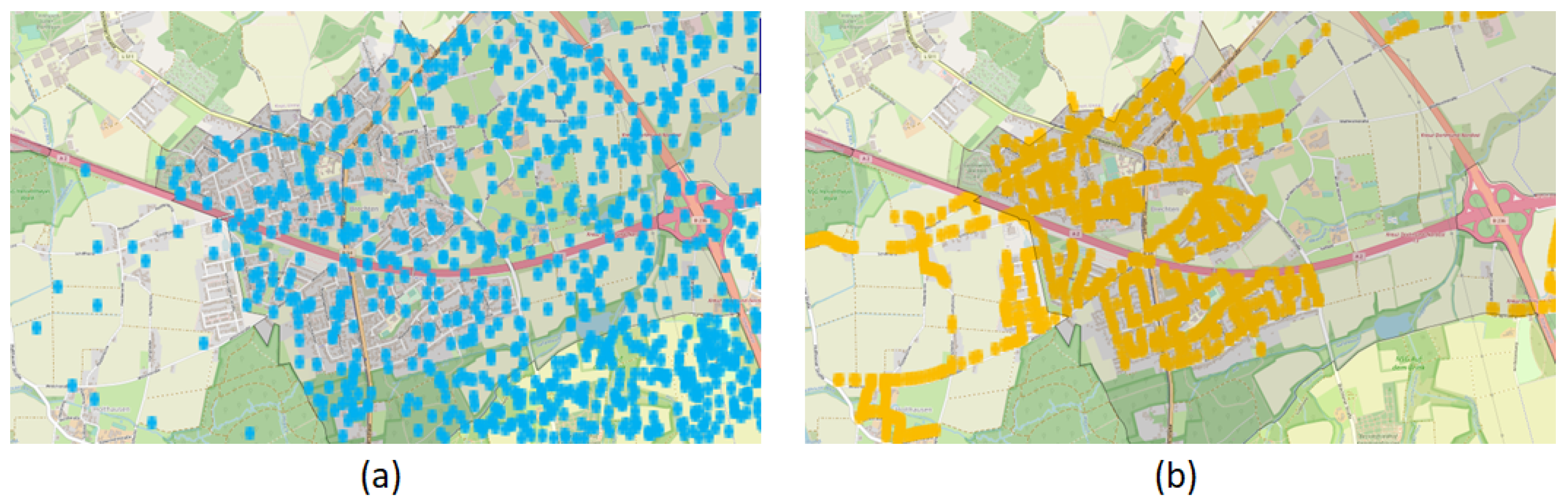
As stated above, solving VRP instances consists of two tasks. Once a cluster of customers is given, the problem is reduced to solving the TSP for each cluster (as defined for the sweep algorithm). For higher accuracy and in order to validate the approximation formula, instances of the TSP could be solved for each tour (minimizing the distance traveled). However, then geographical data for the locations of each transport order are required. Customer locations could be determined randomly within the district area (Figure 3a). As an alternative, real-world data from the open street map (OSM) could be used (Figure 3b) for only importing nodes tagged as residential to obtain realistic points in the area (http://overpass-turbo.eu/ accessed on 1 October 2023). Furthermore, nodes that are too close to other nodes regarding a particular transportation method have been eliminated. The minimum distance between nodes is set to 10 m.
A random selection in the area has the disadvantage that (again) a uniform distribution of points in the area is assumed, which is also the assumption when using Equation (1). In the experiments, the influence of the strategy to select customer locations is further analyzed.
The VKT per area result from the solutions of the respective TSP instances and the journeys from the depot to the respective district area and back (Figure 4). A similar assumption concerning the utilization of tours as for the simple estimation approach needs to be defined. If the number of customers within a district is insufficient to generate only fully-utilized tours, the remaining n nodes are added to the defined neighbor district (which of course has not been planned yet). Here, the closest n nodes are transferred before executing the actual solution method. Only for the last district to be planned, tours not fully utilized are planned. For solving the problem for each district, the following steps are performed:
- the determination of the number of tours per area (according to the capacity of the vehicles).
- the allocation of customers to tours according to the sweep approach (“collecting” customers until the maximum capacity of the vehicle is reached).
- the solving of all TSP-Instances with the construction method Farthest Insertion and the improvement method 2-Opt.
4.3. Solving the VRP for the Overall Problem
Both the sweep (Figure 5a) and the savings method (Figure 5b) have been applied. The objective function applied is to minimize the distance traveled. In order to allow for tackling large problem instances within a reasonable amount of time, the savings list has been reduced to a maximum of four nodes for each node, with the closest node in each direction (north, east, south, and west) being chosen.
5. Modeling APL Systems
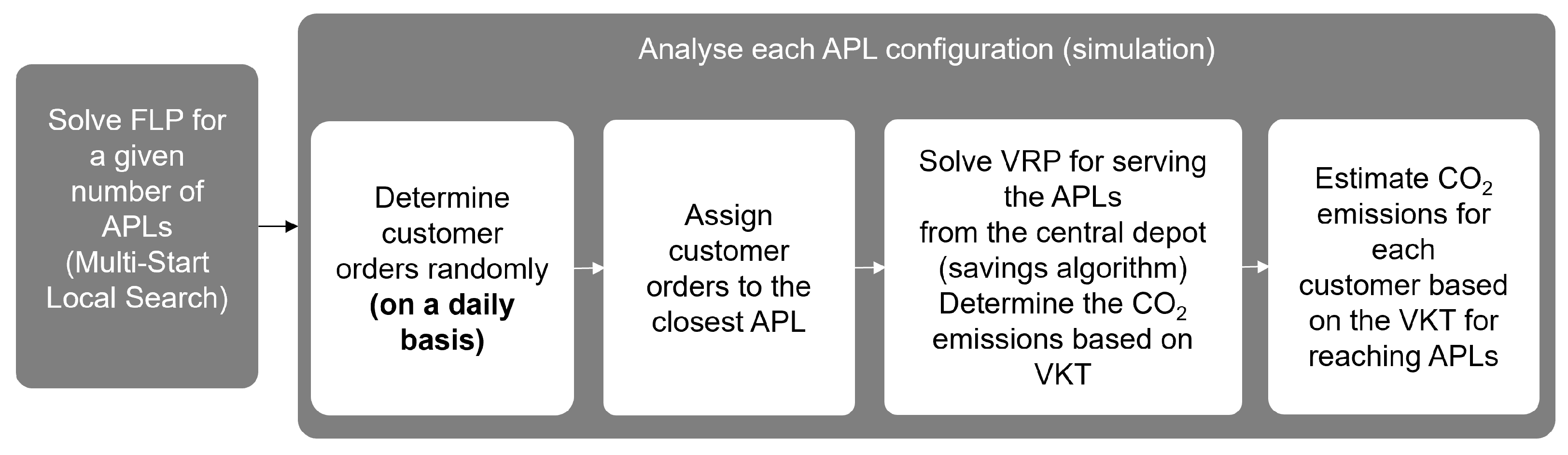
For setting up APL systems, the number and geographical locations of APLs need to be determined. In this context, the proposed solution approach consists of two steps: First, the network configuration is determined solving the underlying FLP for a given number of APLs, i.e., the number of APLs is given as a parameter. The objective function is to minimize the sum of all distances of customers to the assigned APL, and the the result is a list of APLs.
In a second step, each APL configuration is evaluated using a simulation approach. Here, each system configuration under consideration is analyzed by simulating daily orders, the supply transports from the depot to the APLs, and the pickup of parcels by the customers (see Figure 6 for the respective workflow).
5.1. Facility Location Problem
For the FLP, a Multi-Start Local Search has been implemented, i.e., the given number of nodes has been randomly selected and a local search has been performed, where the neighborhood is defined by the n closest nodes of each node. Assuming that each randomly selected customer chooses the closest APL available, each customer is assigned to one of the APL nodes. The objective function is to minimize the sum of all distances of customers to the assigned APL. For each scenario with a given number of APLs, a related structure of an APL system is obtained, which is further analyzed with respect to the operative transport processes in the next step.
5.2. Evaluation of the Transport Processes
In the simulation model, each scenario with its specific APL configuration is further analyzed by randomly generating customer orders for each district. Four different demand scenarios are defined, ranging from about 12,000 to about 26,500 parcels per day in total. In each replication, the given number of parcels is randomly assigned to the possible customer locations derived from the OSM data.
Then, the number of parcels for each APL is determined, assuming that each randomly selected customer chooses the closest APL available. In the next step, the number of full-load transports to the APLs are computed. For the remaining transport quantities, an instance of the respective VRP is formulated and solved using the savings algorithm with the objective to minimize the total distance traveled.
5.3. Consideration of Customer Behavior
For an overall comparison with respect to GHG contribution, the behavior of the customers, i.e., the emissions for picking up parcels at the APL, must also be taken into account. Here, a model is proposed to roughly estimate the additional CO2 emissions. Depending on the distance to the APL, customers walk, take a bike, use public transport, or take a private vehicle to pick up their parcel at the APL. The behavior mainly depends on the distance to the APL and additionally the availability or—more generally—the typical usage of public transport within a certain area or district. Furthermore, a trip is either a single trip from the customer to the APL and back or the customer integrates the stop at the APL into an individual tour, also visiting other locations like shops, restaurants, or the customer’s place of work.
For the options of walking, taking a bike, or using public transport, the assumption is that no relevant additional CO2 emissions have to be considered. In the case of public transport, of course emissions generally arise. In our model, however, we do not assume that new bus or train lines are opened or serve at a higher frequency in order to manage pickups at the APLs. Therefore, no additional CO2 emissions have to be considered for public transport, and the focus lies on the usage of private vehicles. Here, an assumption is required about the percentage of single trips and individual tours. Furthermore, the additional distance taken by the customer when visiting the APL on a tour with further stops has to be estimated. Here, the assumption is that the customer’s tour is extended by the fdt percent of the direct distance to the packing station on average.
The selection of the pickup option for the customers is implemented using a table indicating the probabilities for each pickup option depending on the distance to the APL (Table 1). Given the distance of the customer location to the assigned APL, the respective row is chosen according to column until km. Given the percentage % foot or bike, it is then randomly decided if the customer uses this option for picking up the parcel. If the option is not chosen, it is randomly determined whether the customer uses public transport. According to [60], from all customers that are not traveling by foot or bike, about 28% use public transport. In the cases of tours with the customers’ own vehicles, it is finally randomly determined if they visit the APL with a single trip only for this pickup or during an individual tour combined with other tasks (column % individual tour). If an individual tour is selected, the additional VKT are calculated using parameter fdt as stated above. Otherwise, the VKT are twice the distance of the considered customer to the APL.
As public transport is used to different degrees in the different districts within cities, a correction factor for the percentage of customers using public transport in district i is introduced. Here, the results of a study for the city of Dortmund are used that evaluate the number of transportation methods people used per day (by foot, by bike, using individual vehicles, and using public transport) [60].
The average percentage of public transport was calculated compared to individual vehicles, and parameter is set as the respective factor for the individual deviation compared to the global average value of about 28%. Thus, the respective percentage in Table 1 can be changed, without the necessity to change the individual values for all districts for each scenario to be observed.
A second correction factor is introduced for modeling the influence of the distance to the next public transport stop (bus or train) of a customer. Here, the respective data from OSM are used to determine the distance to the nearest public transport stop for each customer k. The correction factor for each customer k is calculated on the basis of . The values are obtained by mapping to the interval between 0.8 (representing of all customers k) and 1.2 (representing ) of all customers k) with
A correction factor is needed for customers further away from a public transport station as these are less likely to choose public transport in favor of their own car. On the other hand, a correction factor for customers relatively close to a public transport stop leads to a higher probability to choose public transport.
6. Computational Results and Discussion
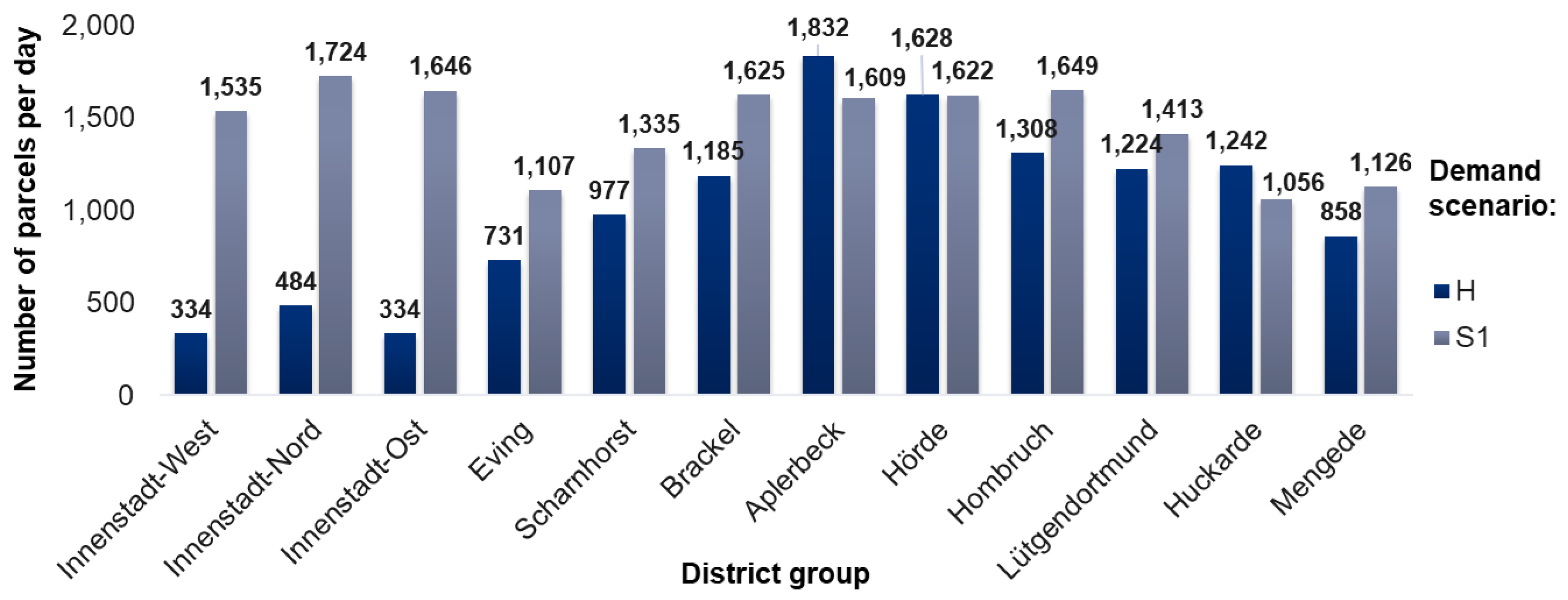
Based on data for the city of Dortmund as a real-world case, a set of experiments has been conducted. Four different scenarios with respect to the daily customer demand for each of the city districts are distinguished. The first demand scenario, denoted as H, is given as real-world data for the number of parcels delivered by the provider Hermes within one week [61]. The other three scenarios, denoted as S1, S2, and S3, correlate to the population of the respective districts, with a growth rate of about 25% for S2 and 50% S3 compared to S1, based on demands presented by [62]. The distribution for the Hermes data is pretty much in line with the other three demand scenarios, with the exception of the inner city, where Hermes obviously does not deliver as many parcels as in the outer districts (Figure 7). An additional assumption is that all customer orders are available at the beginning of the day and transport routes are not re-optimized during the day.
6.1. Direct Deliveries
In a first experiment, the indicator VKT for the distribution of all parcels is computed for direct deliveries. Three different levels of aggregation have been presented in Section 4. First, results are presented from comparing the estimation approach based on the sizes of the area and solving TSP instances for customers within a given area.
6.1.1. Area-Based Approaches
As stated above, mainly full-truck loads are assumed, i.e., tours are sequentially planned for all city districts. The results are given in Table 2. Column VKT DC to the Center of the Districts and Back gives the distances for driving from the DC to the respective centers of the districts and back to the DC. These distances need to be added to the distances traveled on the tours within each district.
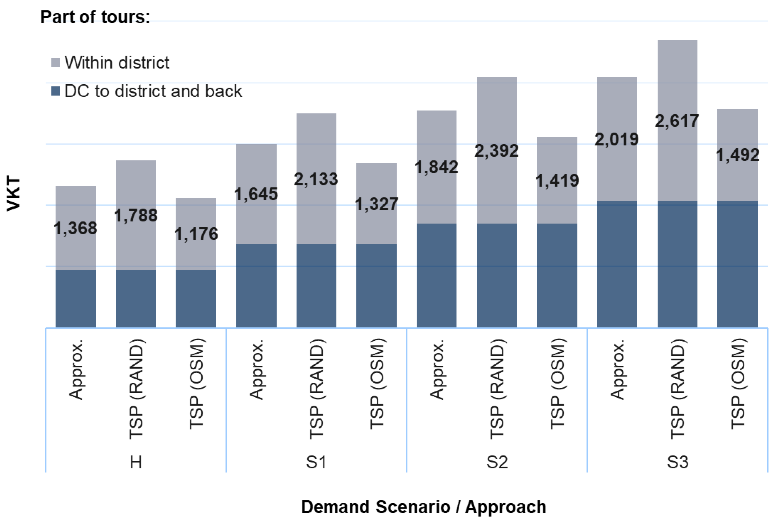
The kilometers traveled within each district are first estimated on the basis of Equation (1) for each district, denoted as Approx. in Figure 8. In order to validate these results, they are compared to actually solving the TSP for respective customer locations and orders. Here, two different settings for the underlying data sets are distinguished, a random selection of customer locations, denoted as TSP (RAND) and using nodes from open street map, denoted as TSP (OSM).
The results show a high impact of the choice of data sets for the example of Dortmund (see Figure 8). In all scenarios, the sum of VKT is about 23% less for the TSP approach with fixed regions when using the OSM data compared to randomly generated data sets. This is due to the relatively high degree of areas in Dortmund where no residents live.
The choice of data for customer locations also has a significant effect when looking at the results for the approximation approach, where Equation (1) either leads to too optimistic (RAND) or pessimistic (OSM) results. When actually solving TSP instances in the respective districts, a deviation of 11% is obtained when assuming OSM data, and −16% for randomly generated customer locations compared to the simple approximation approach. As a result, further studies should rely on more realistic data (as given by OSM), and one should always carry out tests before possibly integrating approximation approaches. Here, the original correction factor of 0.765 in Equation (1) could be changed in order to obtain more realistic results.
6.1.2. Solving VRP Instances for All Customers under Consideration
The savings algorithm performs better than the TSP approach (presented in the previous section) with predefined areas and also better than the sweep algorithm for almost all demand scenarios, mainly due to larger areas without residents, which have to be traveled through on more tours using the sweep algorithms than for the savings algorithm (Table 3).
For all scenarios, the VKT are also about 23% less for the savings algorithm when using the OSM data compared to randomly generated data sets. For the sweep algorithm, only a reduction in VKT of 10 to 15% can be observed.
6.2. APL Systems
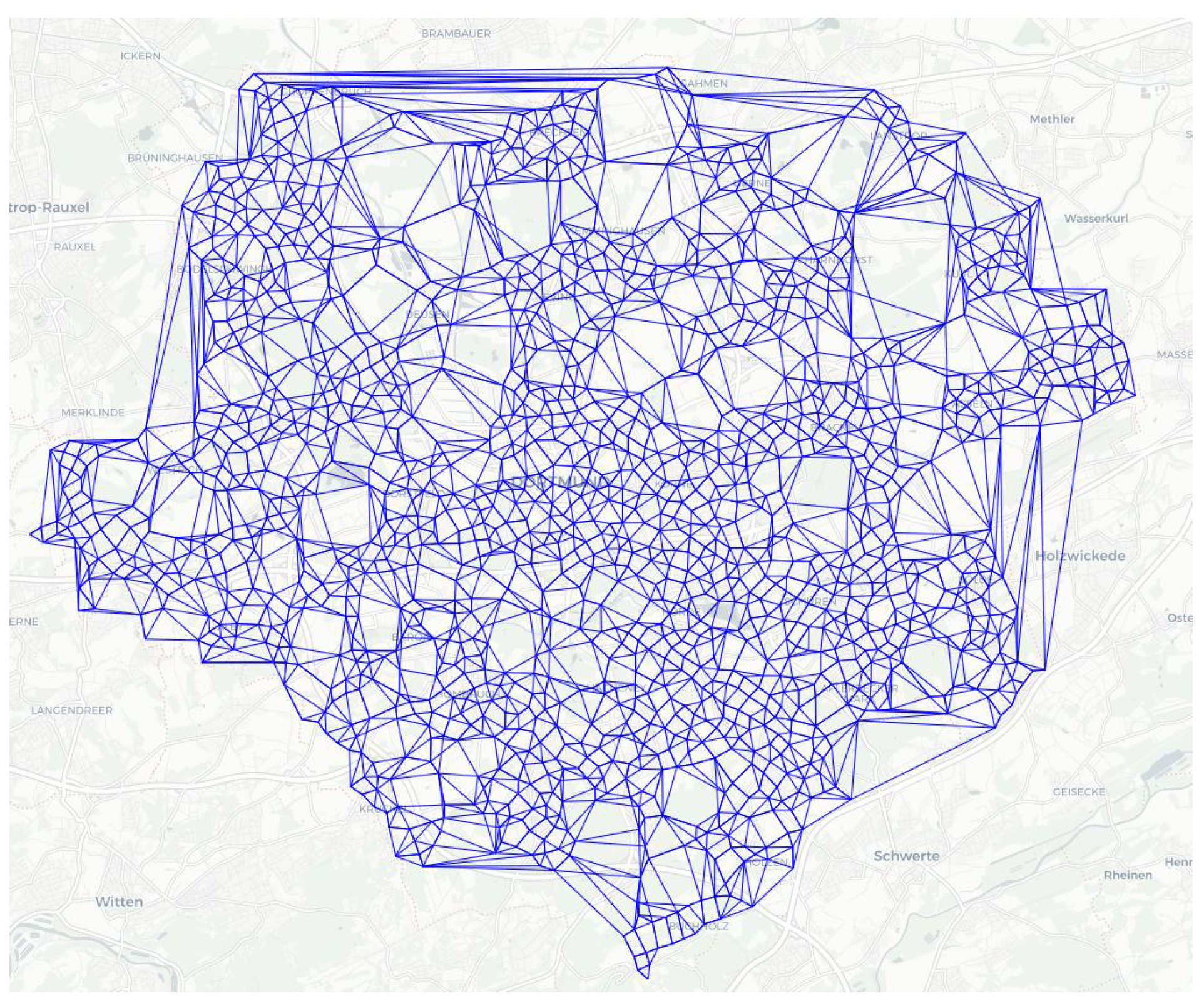
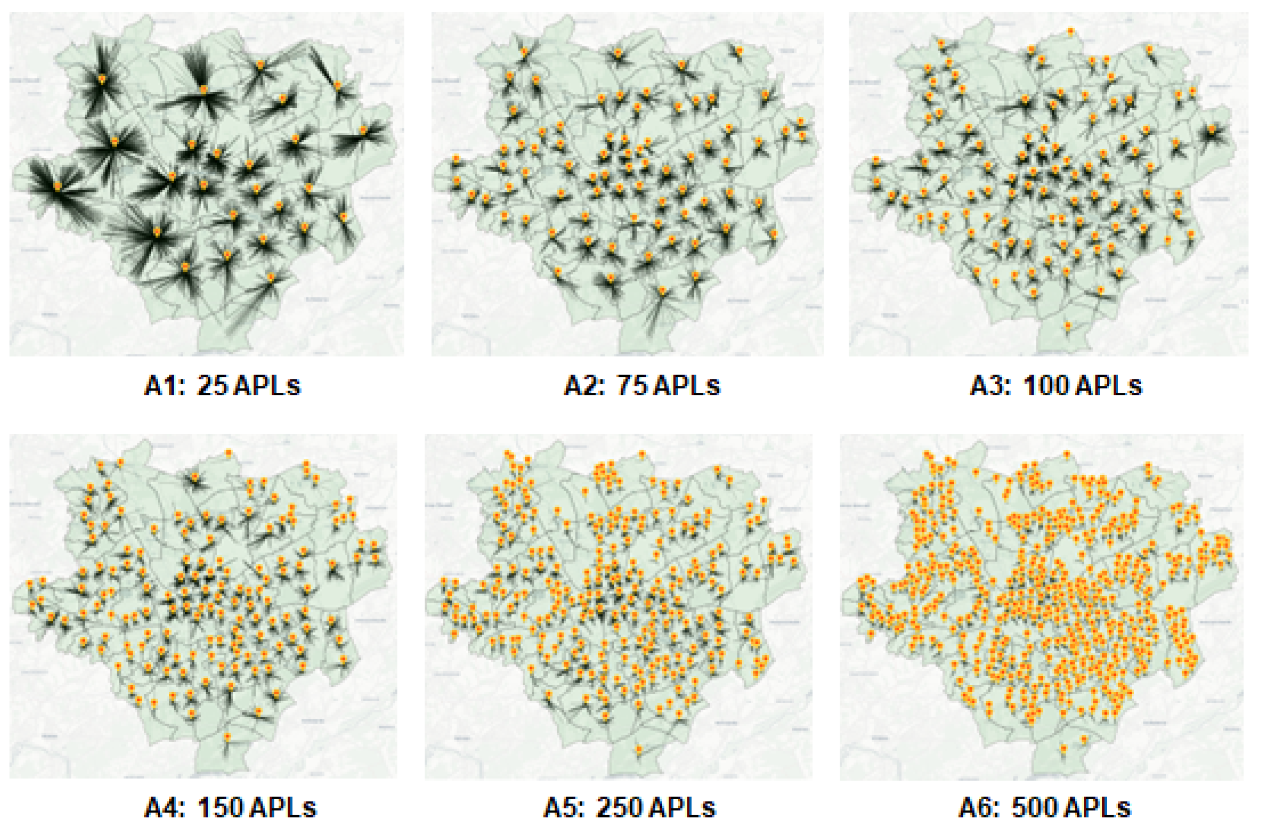
To enable the experiments to analyze APL systems, six different scenarios for the number of APLs have been defined ranging from 25 APLs (scenario ) to 500 APLs (scenario ). For the possible locations of APLs, about 1500 nodes have been selected from the given OSM data tagged as residential, ensuring that each APL has a minimum distance to all other possible APL locations of 200 m (Figure 9 for the resulting neighborhood structure of the FLP).
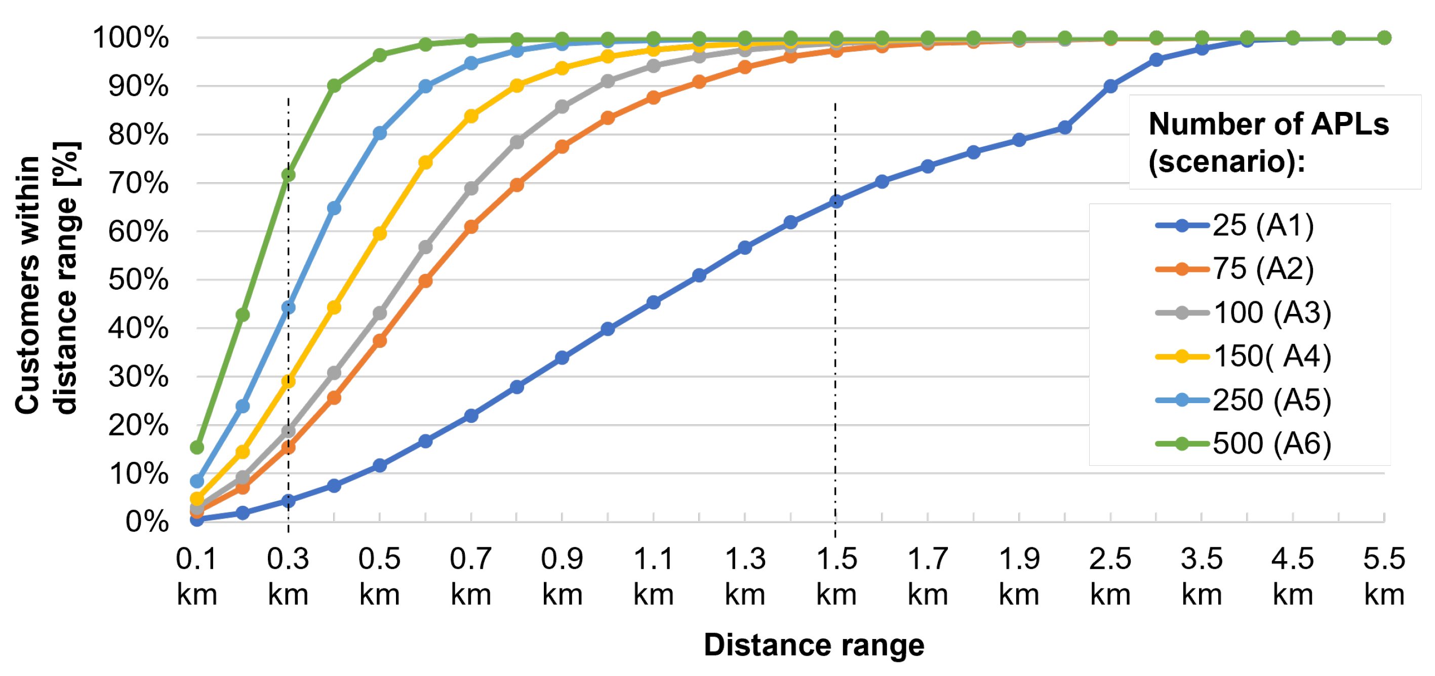
The resulting structures after solving the underlying FLP with about 10,500 randomly selected customer locations from the OSM data set are illustrated in Figure 10 for all six APL scenarios. In Figure 11, an evaluation of the distances to the APLs is presented. Only 4% of all customers are assigned to an APL within a distance of 300 m for scenario (under the assumption that customers always walk or take a bike to the respective APL). Even in scenario A6 with 500 APLs, only 72% of all customers are assigned to an APL within a distance radius of 300 m. About 66% of the customers are within a radius of 1.5 km to their nearest APL. For all other scenarios, A2 to A6, almost all customers are within that radius, ranging from 97% (A2) to 100% (A5 and A6).
Each APL configuration is further evaluated on the basis of the four given demand scenarios H, S1, S2, and S3. Solving the VRP for all transports from the distribution center (DC) to all APLs leads to the results given in the Appendix A (Table A1). Depending on the capacity of the vehicles C, the numbers of tours are within a range of 46 (H–A1) to 110 tours (S3–A6) for and 20 to 55 tours for , respectively.
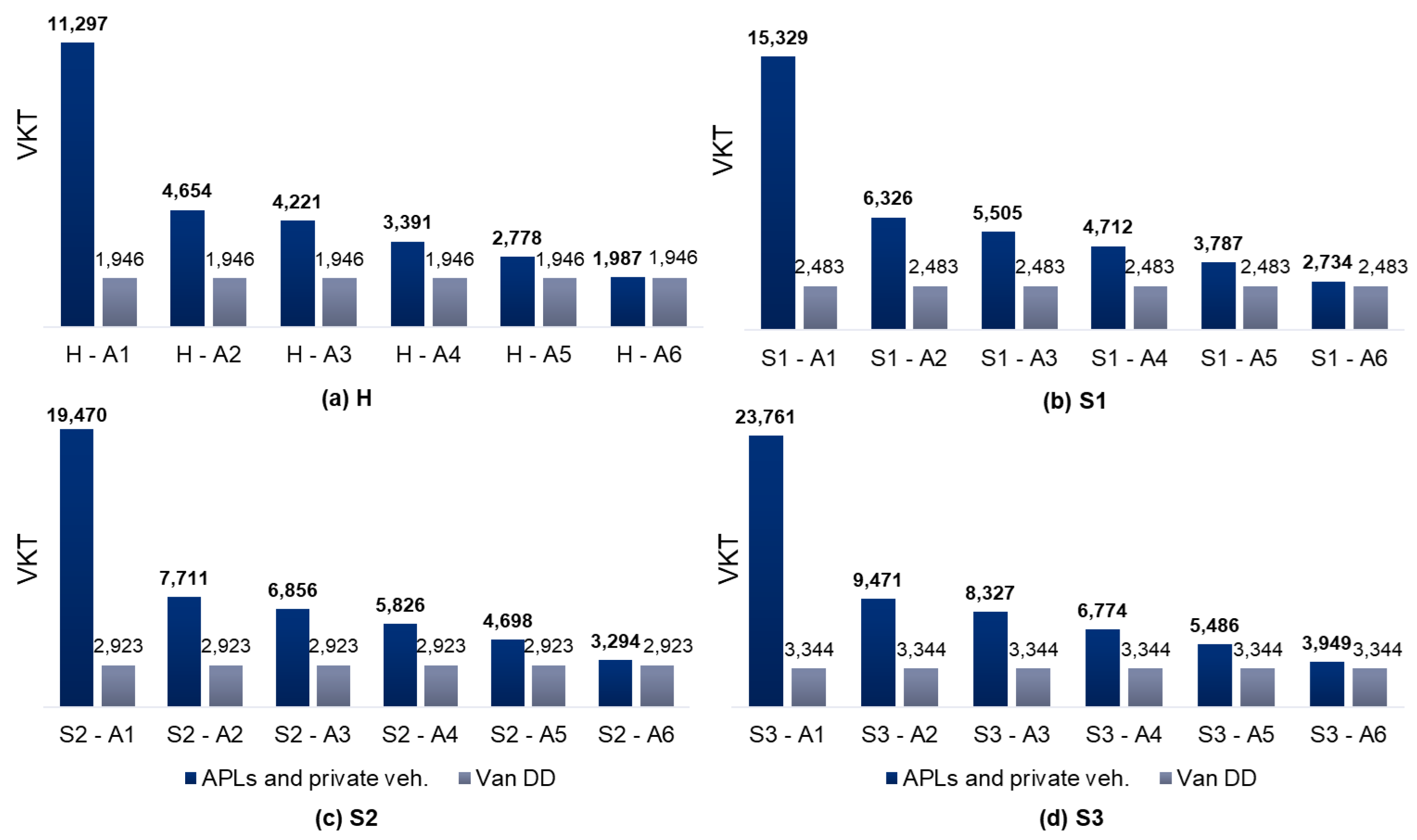
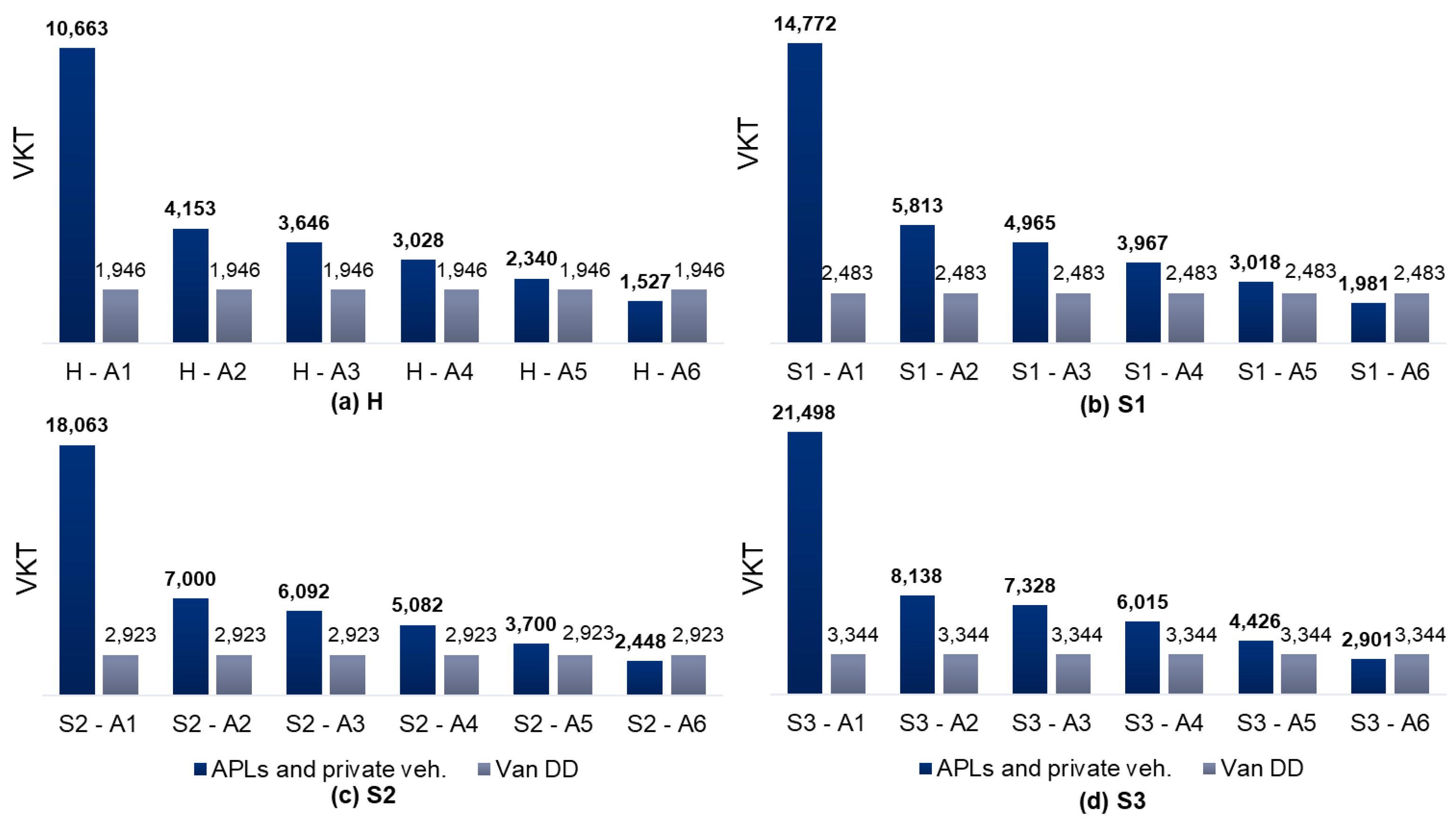
The sum of VKT from the DC to the APLs as full truck loads (FTL) and VKT of tours serving more than one APL is typically much smaller than for DD. However, the VKT of customers also needs to be considered when comparing the results for the different scenarios. Following the approach presented with the parameter settings given in Table 1, the DD (the minimum VKT of the respective results of the savings and the sweep algorithm) leads to less VKT for all scenarios for a capacity of the vehicles (Figure 12). Only for scenarios H–A6 are nearly comparable results achieved with a deviation of about 2%. If the capacity of the vehicles is set to , better results than for direct deliveries are obtained for the APL scenario A6 for all four demand scenarios (Figure 13), ranging from savings in VKT from 21% (H) to 15% (S3), compared to DD given in the Appendix A (Table A2).
For demand scenario H, full trucks can only be planned for APL scenarios A1–A3. For scenario A1, the ratio of the distance traveled as full-truck tours is 68%, while for A3 this ratio is only 19%. For the largest demand scenario S3, 87% of the distance for serving APLs is completed as full-truck tours for scenario A1 with 25 APLs, while for scenario A5 this ratio is 7%.
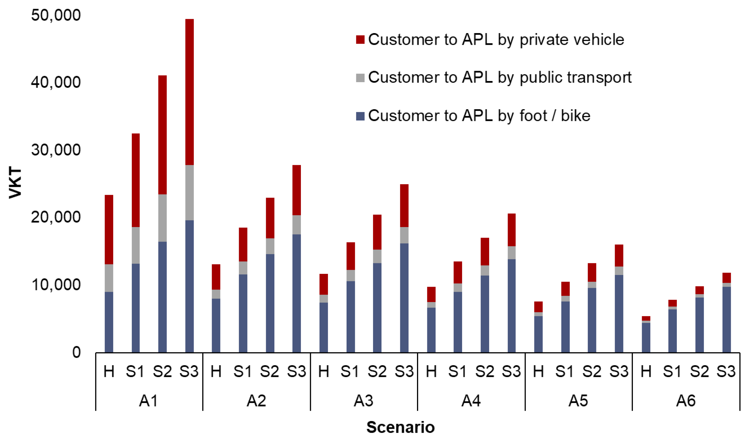
In Figure 14, the distances traveled by customers are given, which distinguish the three different options of traveling to the APL. The more APLs are introduced, the lower the total distances for customers are. Additionally, the ratio of distances traveled by private vehicles is significantly reduced when introducing more APLs. For APL scenario A1 with 25 APLs, the ratio is 43.4% on average; for A4 with 150 APLs, the ratio is 23.6%; and for A6 with 500 APLs, the ratio is 12.6%. The variance with respect to the different demand scenarios is very small for all APL scenarios.
The VKT for each APL configuration has been evaluated for the four demand scenarios H, S1, S2, and S3. Table A2 in Appendix A provides detailed results. Figure 12 presents a comparison of VKT metrics for APL systems, including VKT for private vehicles and DD, with a value of C = 250. Our analysis clearly shows that in all scenarios the A1 configuration, featuring 25 APLs within the urban setting, exhibits the highest VKT. This can be attributed to the inadequacy of APLs for parcel pickup through more efficient means such as cycling or walking, which forces customers to cover longer distances using private vehicles. When assessing the A1 APL configuration, it becomes apparent that DD demonstrates remarkable efficiency gains, with improvements of 480%, 517%, 566%, and 611% for the Hermes, S1, S2, and S3 scenarios, respectively. Furthermore, across all additional configurations (A2, A3, A4, A5, and A6), DD consistently exhibits lower VKT in comparison to using APLs in conjunction with private vehicles for parcel pickup. In Figure 13, we examine a comparison of VKT metrics for APL systems, maintaining a value of C = 500. The trends persist consistently throughout the analysis. Notably, it becomes evident that the maximum advantage peaking at 22% over DD can be observed up to the A6 configuration, which comprises 500 APLs.
6.3. CO2 Results Comparison
In order to ensure the realism of our results, we have carefully calculated the fuel consumption, taking into account the technical specifications of one of the most widely used commercial vehicles for last-mile transport, namely, the Mercedes-Benz Sprinter Cargo 311 CDI kompakt van. This van has the same engine as its counterpart for passenger transport. Based on the available technical data, the Mercedes-Benz Sprinter Cargo van has fuel consumption and CO2 emissions of 9.6 l/100 km and 247 gCO2/km, respectively. For more details on the official fuel consumption and specific CO2 emissions, refer to [63]. For calculating the fuel consumption of private cars, we have been guided by the average consumption of regular gasoline and diesel in Germany (with a split of about two thirds regular and one third diesel), which results in about 7.5 l/100 km on average [64,65]. As far as emissions are concerned, the value is based on a baseline of 178 gCO2/km [66].
Building upon the previous section, we conduct an evaluation of each APL configuration. This comprehensive assessment is rooted in the technical data related to both fuel consumption and emissions, and it extends across the four specified demand scenarios H, S1, S2, and S3.
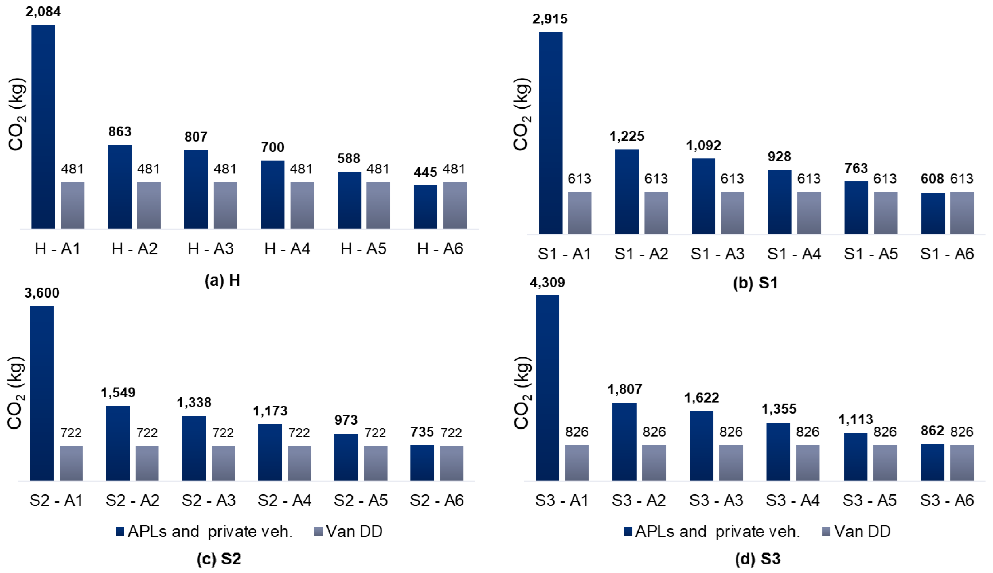
The evaluation of CO2 emissions for the APL configurations has been conducted for the four demand scenarios, with detailed results provided in Appendix A (Table A3). Figure 15 offers a comparison of CO2 metrics for APL systems for private vehicles and DD, with a constant parameter value of C = 250. Our analysis indicates a consistent trend regarding CO2 emissions. In all scenarios, the A1 configuration, featuring 25 APLs, exhibits the highest emissions. When assessing the A1 APLs configuration, it becomes evident that DD demonstrates significant efficiency gains, with improvements of 334%, 375%, 399%, and 422% for the Hermes, S1, S2, and S3 scenarios, respectively. Across configurations A2, A3, A4, and A5, DD consistently results in lower CO2 emissions compared to using APLs in conjunction with private vehicles for parcel pickup. However, it is noteworthy that only in the A6 configuration is APL usage more efficient, with a maximum advantage of 4%.
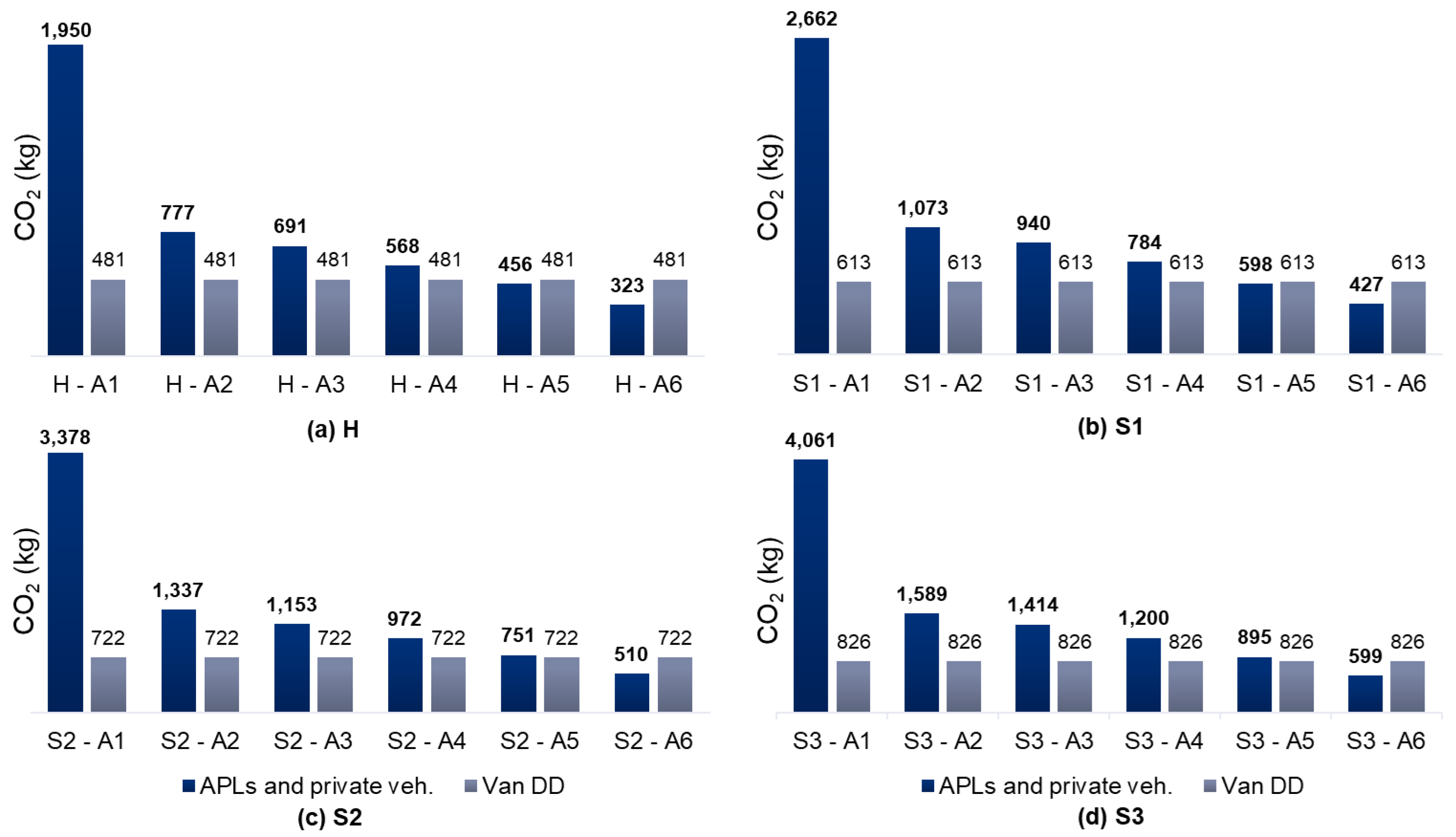
Figure 16 presents a comparison of CO2 metrics for APL systems, maintaining a value of C = 500 given in Appendix A (Table A4). The observed trends remain consistent for APL scenarios A2, A3, and A4. Notably, it becomes evident that in scenarios A5 and A6, the advantage of using APLs over DD ranges between 13% and 22%.
In comparing APLs and DD in terms of CO2 emissions, the results, considering customer behavior, offer a comprehensive assessment. APL systems have operational cost advantages, but to keep emissions comparable to DD, the city of Dortmund needs a minimum of 250 APLs, as per the A5 and A6 scenario results.
In the last experiment, a sensitivity analysis has been conducted. For three different parameters (ratio foot or bike, ratio public transport, and ratio individual tour) from Table 1, an iterative increase in the parameter value (with an increment of one percentage point) is analyzed until a better result (in terms of CO2 emissions) than for direct deliveries is achieved.
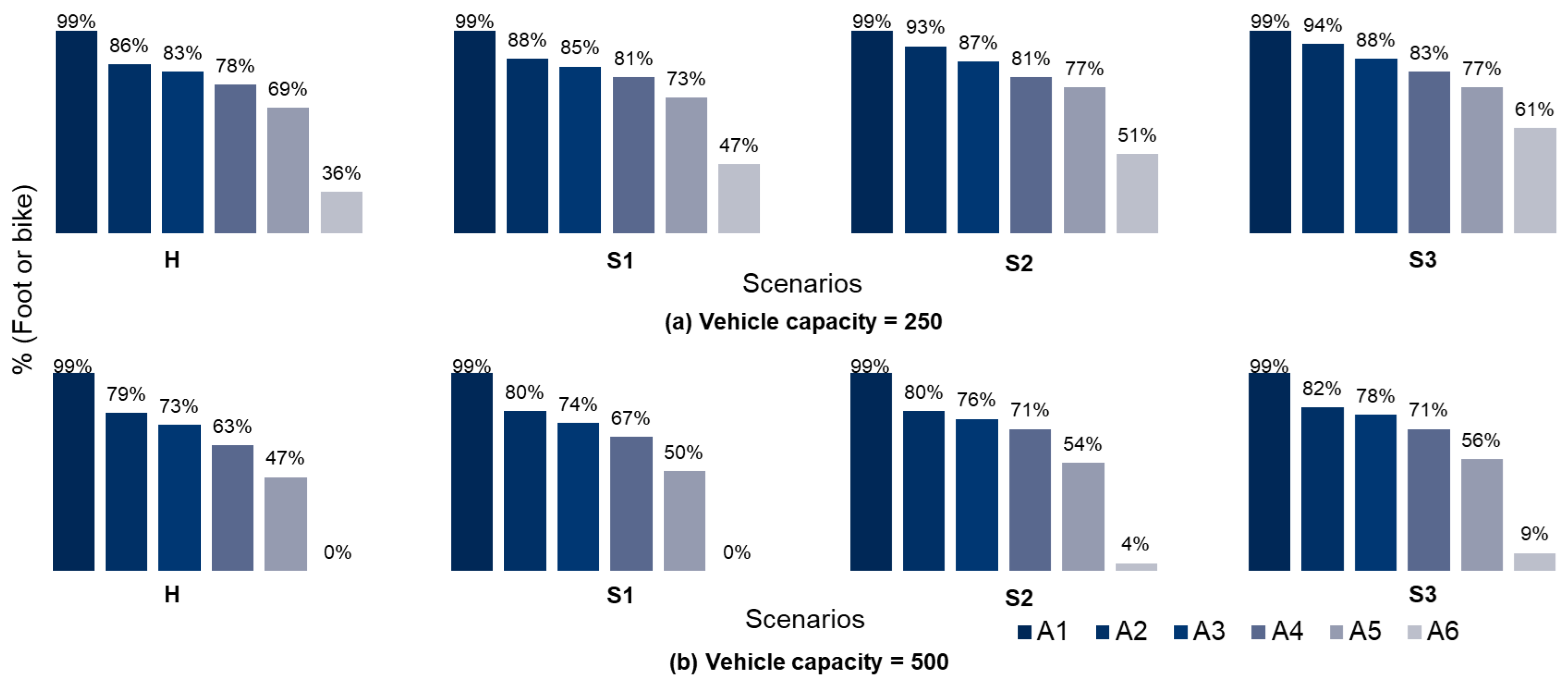
In Figure 17, the results for increasing the percentage of customers (with a distance between 0.3 and 1.5 km to the nearest APL) picking up their parcels by foot or bike are given. For scenario A1, no superior results can be obtained, even if the respective parameter is set to 99% (as indicated in the figure). For all other APL configurations, a parameter setting can be determined where the APL system leads to fewer CO2 emissions than DD. The more APLs that are introduced and the higher the capacity of the vehicle serving the APLs, the lower the respective break-even point for the considered parameter ratio by foot or bike is. Furthermore, it can been observed that along with higher demand, the percentage of customers picking up their parcel by foot or bike needs to be further increased (for all APL configurations) to achieve better results than for direct deliveries.
With respect to the original assumption of 50% by foot or bike, for a vehicle capacity of 250 parcels (serving the APLs) only the APL configuration A6 is below or within a closer range, with 36% for demand scenario H and up to 61% for scenario A6 (Figure 17a). Increasing the vehicle capacity to 500 parcels leads to a different picture. Here, configuration A6 would lead to better results than DD, even if only a very small percentage (at most, 9% of the customers for scenario (S3) would walk or take a bike to pick up their parcel, with a distance between 0.3 and 1.5 km (Figure 17b)). In this case, APL configuration A5 also leads to comparable results with a percentage of customers, with a distance between 0.3 and 1.5 km to the nearest APL that pick up their parcels by foot or bike ranging between 47% (H) and 56% (S3) as a break-even point. When introducing less than 250 APL locations (A1–A4), better results can only be obtained if the percentage is much higher than the assumed 50%.
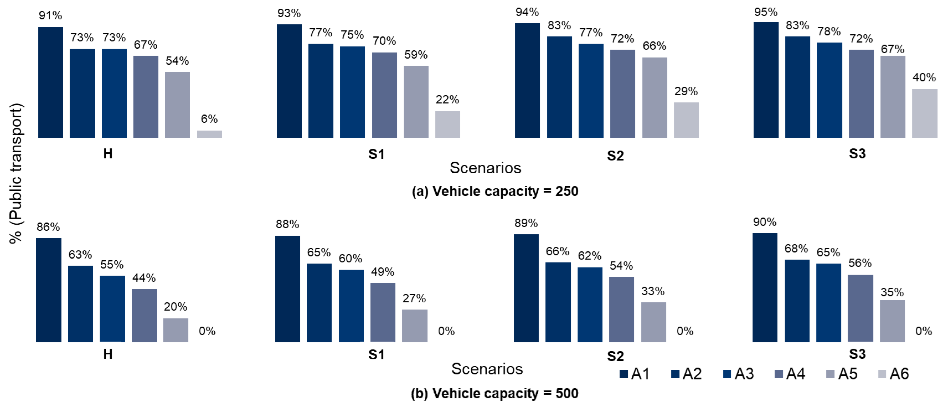
Similar trends can be observed when increasing the ratio of customers choosing public transport instead of a private vehicle (Figure 18). Here, the impact is higher than for the first parameter observed, as for all APL system configurations a parameter setting can be found that leads to superior results for all APL scenarios, with the exception of A1. For ALP configuration A1 and demand scenario S3, however, 95% of customers (not already walking or taking a bike to reach the APL location) would have to choose public transport instead of a private car, which is not a realistic assumption. As currently only about 28% of the citizens of Dortmund choose public transport instead of private vehicles, again only scenario A6 is within a realistic range for a vehicle capacity of 250 parcels (Figure 18a), with a parameter range between only 6% (H) and 40% (S3). For a vehicle capacity of 500 parcels, APL configuration A5 also leads to comparable results, with the break-even point ranging from 20% (H) to 35% (S3).
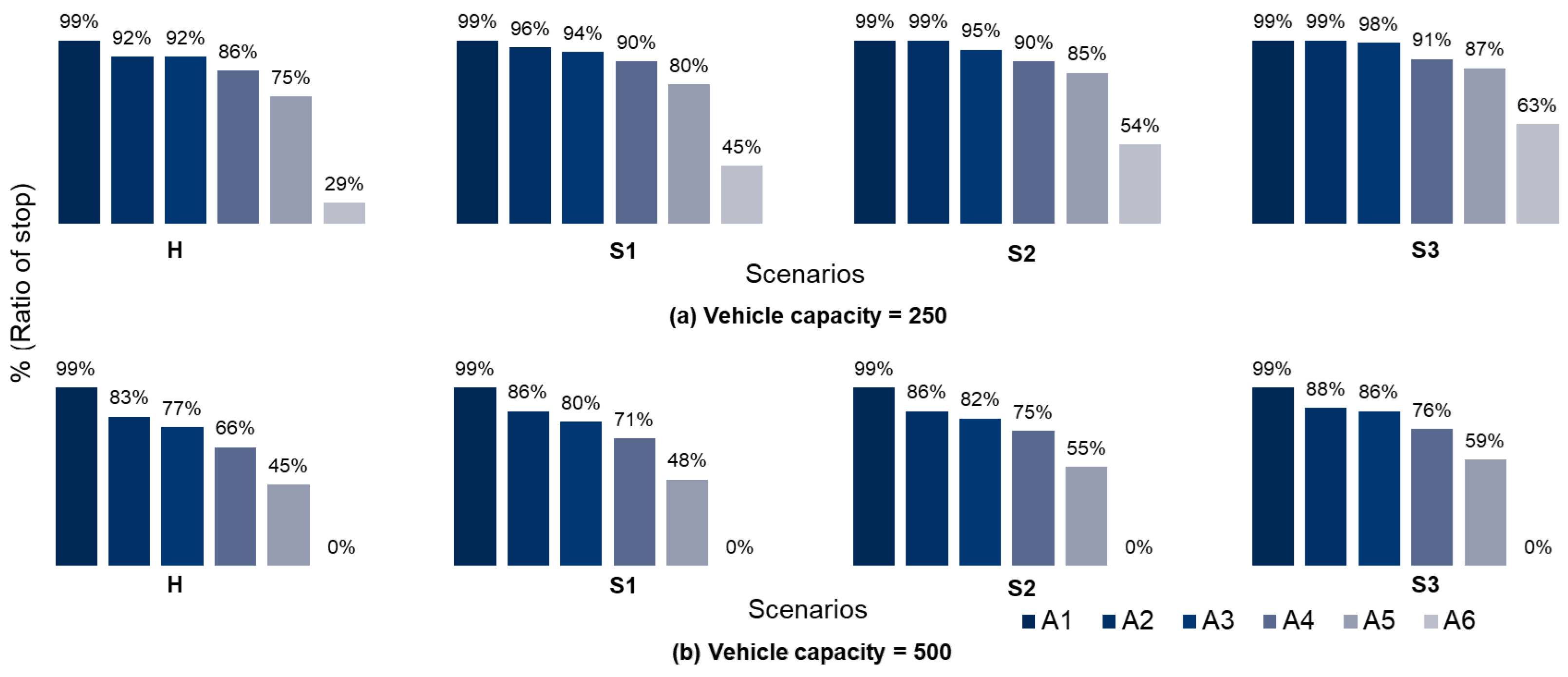
In Figure 19, the results for the sensitivity analysis for the parameter ratio of APL as a stop on an individual tour are given. Here, the respective break-even points are relatively high for most scenarios. For APL configuration A1, no comparable results can be obtained, even if 100% of all customers picking up parcels at the APL location by car do this as part of an individual tour (for both capacity configurations of the vehicles serving the APLs from the central depot).
For demand scenario S3, superior results for the APL systems can be found for APL configuration A6 for a vehicle capacity of 500 parcels. For a vehicle capacity of 250, for demand scenarios S2 and S3 the percentage has to be higher than the originally assumed 50% to obtain better results for the APL configuration A6. For APL configuration A5, comparable results can be obtained for a vehicle capacity of 500 parcels, with values ranging from 45% (H) to 59% (S3). For all other APL configurations with 150 APL locations or less, the percentage of customers picking up parcels as part of an individual tour needs to be between 68% and 98% to reach the break-even point in comparison to direct deliveries (depending on the respective scenario).
7. Conclusions
In this paper, an approach has been presented to compare direct deliveries (DD) with APL systems for last-mile deliveries in larger cities. For the evaluation of DD, three different levels of detail have been compared. The results show that further studies should not only rely on simple formulas to estimate the distances traveled for distribution. At least correction factors should be verified or estimated anew for each given problem instance. Such a verification should be performed on the basis of rather detailed models, with respect to both the underlying data for customer locations and the planning methods applied to generate tours. The results presented show that using data from the open street map (OSM) leads to significantly different, here shorter, tour lengths than using random data within the given areas. Furthermore, further studies should model the methods used for planning tours for vehicles according to the actual situation for the given problem instance. As in practical cases, often Vehicle Routing Problems are solved using heuristics; these approaches, such as the savings algorithm and further improvements methods, which have also been applied in this paper, should be implemented.
With respect to the comparison of APL systems and DD on the basis of CO2 emissions, the results show that it is necessary to also model the customer behaviour to reach APL locations for a fair and profound comparison. It is, of course, favorable for logistic providers to use APL systems in terms of operational costs as less distance has to be traveled compared to dropping off each parcel at the customer location. The savings range from 30% to 90% for different scenarios, which are in line with the findings of previous works presented in Section 2.2.
However, also taking distances traveled by customers by car to reach the APLs into account leads to a completely different picture. As a conclusion, APL systems are only competitive with direct deliveries if a sufficient number of APLs are introduced and more customers pick up their parcels with zero emission (by foot or bike). In the results presented, a system with 250 APLs leads to lower emissions than DD for most demand scenarios, if the capacity of the vehicle serving the APLs is set to 500. These findings are nearly in line with the results presented by [47], who conclude that APL systems are competitive in urban areas if the distance a customer must travel by car to reach the APL is within 0.94 km. As shown in Figure 11, for APL configurations A5 and A6, which lead to better results than direct deliveries in most demand scenarios, nearly 100% of all customers are within this radius. In comparison, for A4 (150 APLs), only about 95% of all customers are within that distance range, and direct deliveries lead to better results in all demand scenarios.
Setting the parameters correctly is one of the most challenging tasks for using the proposed model as the ratios for the different means of transport for customers in dependence of the distance to be traveled are only roughly estimated. Here, conducting a sensitivity analysis is a possible way to check the robustness of the results. Our results for the sensitivity analysis show that typically the different factors need to be increased by a high—and rather unrealistic—degree to obtain different results than in the standard parameter settings proposed. This leads to the conclusion that the results obtained can be rated as robust, even though only one parameter has been analyzed at a time. Future research could focus on a broader design of experiments, with two or more parameters analyzed at the same time.
Besides the problem of valid parameter settings of the model, there are further limitations set in the modeling approach. The possible positions of APLs have been determined randomly, and the actual road network has not been modeled in detail. Instead, the distances between two locations have been approximated on the basis of the air-distance. Along with that, dynamically occurring traffic delays, which typically lead to higher fuel consumption, have not been considered. For direct deliveries, no-shows have not been considered either, typically leading to a higher number of orders for the following day or the need for a re-optimization on the same day.
Nonetheless, the model presented is a good basis for determining a reasonable number of APLs to be set up such that CO2 emissions are comparable to direct deliveries. Of course, combined delivery processes (as indicated in Figure 1b), where tours serve both customers directly and APLs for areas where customers are relatively close to APLs, offer the possibility to gain improvements compared to only serving customers directly. But as a basis, it is highly interesting to also analyze the two distribution options DD and APL as stand-alone options.
8. Further Research
The modeling approach and the resulting simulation model should be used to also analyze other cities to further validate the model and compare the respective results. First progress has been reported by [67] for the city of Pamplona (Spain).
For future research, different issues could be tackled. The OSM data could be analyzed in greater detail in order to map the population to actual houses instead of nodes in the road network. Here, even higher accuracy could be expected. Furthermore, for direct deliveries, a more-detailed simulation model could be defined, including a re-optimization of tours with respect to orders that have not been completed due to customers not being at home.
For further research, the authors will also concentrate on combined tours including DD and APL orders in order to gain more insight into efficient combinations of both delivery types. For this purpose, the originally addressed facility location problem needs to be redefined as only a subset of all customers would be assigned to APLs. Here, instances of the Maximal Covering Location Problem could iteratively be defined (with different parameter settings), such that nearly optimal numbers and geographical locations of APLs with respect to CO2 emissions could be determined on the basis of the different demand scenarios.
For overall decisions on the configuration of APL systems, there are other factors that are important to consider, such as delivery time, cost-effectiveness, and customer satisfaction. In this context, analyzing CO2 emissions is only one part of the overall decision process, and future research could also concentrate on defining respective multi-criteria optimization models.
Author Contributions
Conceptualization, K.G., M.R. and J.C.-V.; methodology, K.G. and J.C.-V.; software, K.G.; validation, K.G., M.R. and J.C.-V.; formal analysis, M.R. and K.G.; writing—original draft preparation, J.C.-V. and K.G.; and writing—review and editing, M.R. and K.G. All authors have read and agreed to the published version of the manuscript.
Funding
This work was partially supported by the Center for International Migration (GIZ/CIM) Grants–Return Expert Programme (2021–2023) at German Federal Ministry for Economic Cooperation and Development (BMZ).
Data Availability Statement
Data are available upon reasonable request to the corresponding author.
Conflicts of Interest
The authors declare no conflicts of interest.
Appendix A. Direct Deliveries and APL Systems: Comparative Results

Table A1.
Comparison of VKT by customers per day for the different options.
| Scenario | VKT Cust. Foot/Bike | VKT Cust. Pub. Transp. | VKT Cust. Vehicle | VKT Veh. C = 250 | VKT Veh. C = 500 | VKT Veh. DD | Dev C = 250 [%] | Dev C = 500 [%] |
|---|---|---|---|---|---|---|---|---|
| H–A1 | 9000 | 4082 | 10,324 | 11,297 | 10,663 | 1946 | 480 | 448 |
| H–A2 | 8107 | 1399 | 3693 | 4654 | 4153 | 1946 | 139 | 113 |
| H–A3 | 7452 | 1206 | 3115 | 4221 | 3646 | 1946 | 117 | 87 |
| H–A4 | 6438 | 925 | 2231 | 3391 | 3028 | 1946 | 74 | 56 |
| H–A5 | 5408 | 604 | 1552 | 2778 | 2340 | 1946 | 43 | 20 |
| H–A6 | 4441 | 280 | 686 | 1987 | 1527 | 1946 | 2 | −22 |
| S1–A1 | 13,002 | 5445 | 13,904 | 15,329 | 14,772 | 2483 | 517 | 495 |
| S1–A2 | 11,279 | 1978 | 5009 | 6326 | 5813 | 2483 | 155 | 134 |
| S1–A3 | 10,623 | 1592 | 4088 | 5505 | 4965 | 2483 | 122 | 100 |
| S1–A4 | 9159 | 1261 | 3216 | 4712 | 3967 | 2483 | 90 | 60 |
| S1–A5 | 7640 | 794 | 2146 | 3787 | 3018 | 2483 | 53 | 22 |
| S1–A6 | 6430 | 374 | 1006 | 2734 | 1981 | 2483 | 10 | −20 |
| S2–A1 | 16,226 | 6947 | 17,701 | 19,470 | 18,063 | 2923 | 566 | 518 |
| S2–A2 | 14,366 | 2374 | 5972 | 7711 | 7000 | 2923 | 164 | 140 |
| S2–A3 | 13,280 | 2025 | 5146 | 6856 | 6092 | 2923 | 135 | 108 |
| S2–A4 | 11,393 | 1566 | 4105 | 5826 | 5082 | 2923 | 99 | 74 |
| S2–A5 | 9538 | 1042 | 2715 | 4698 | 3700 | 2923 | 61 | 27 |
| S2–A6 | 8037 | 474 | 1213 | 3294 | 2448 | 2923 | 13 | −16 |
| S3–A1 | 19,902 | 8145 | 21,622 | 23,761 | 21,498 | 3344 | 611 | 543 |
| S3–A2 | 17,333 | 2919 | 7405 | 9471 | 8138 | 3344 | 183 | 143 |
| S3–A3 | 15,965 | 2447 | 6366 | 8327 | 7328 | 3344 | 149 | 119 |
| S3–A4 | 13,800 | 1929 | 4851 | 6774 | 6015 | 3344 | 103 | 80 |
| S3–A5 | 11,502 | 1305 | 3236 | 5486 | 4426 | 3344 | 64 | 32 |
| S3–A6 | 9755 | 583 | 1492 | 3949 | 2901 | 3344 | 18 | −13 |
Table A2.
Comparison of VKT and number of tours from the DC to the APLs.
| Scenario | VKT to APLs VRP (C = 250) | VKT to APLs FTL (C = 250) | # Tours VRP (C = 250) | # Tours FTL (C = 250) | VKT to APLs VRP (C = 500) | VKT to APLs FTL (C = 500) | # Tours VRP (C = 500) | # Tours FTL (C = 500) |
|---|---|---|---|---|---|---|---|---|
| H–A1 | 295 | 678 | 10 | 36 | 339 | 92 | 12 | 8 |
| H–A2 | 699 | 262 | 32 | 10 | 608 | 0 | 25 | 0 |
| H–A3 | 893 | 213 | 38 | 10 | 641 | 0 | 26 | 0 |
| H–A4 | 1160 | 0 | 50 | 0 | 667 | 0 | 26 | 0 |
| H–A5 | 1226 | 0 | 50 | 0 | 714 | 0 | 25 | 0 |
| H–A6 | 1300 | 0 | 50 | 0 | 806 | 0 | 25 | 0 |
| S1–A1 | 327 | 1098 | 11 | 57 | 333 | 375 | 12 | 22 |
| S1–A2 | 754 | 563 | 34 | 28 | 774 | 0 | 35 | 0 |
| S1–A3 | 959 | 458 | 42 | 24 | 807 | 17 | 35 | 1 |
| S1–A4 | 1362 | 134 | 60 | 8 | 888 | 0 | 38 | 0 |
| S1–A5 | 1641 | 0 | 73 | 0 | 919 | 0 | 37 | 0 |
| S1–A6 | 1729 | 0 | 73 | 0 | 998 | 0 | 36 | 0 |
| S2–A1 | 302 | 1467 | 10 | 76 | 321 | 496 | 11 | 29 |
| S2–A2 | 709 | 1030 | 31 | 49 | 791 | 54 | 36 | 2 |
| S2–A3 | 963 | 747 | 43 | 38 | 880 | 74 | 39 | 3 |
| S2–A4 | 1425 | 296 | 63 | 16 | 1048 | 0 | 45 | 0 |
| S2–A5 | 1922 | 61 | 86 | 4 | 1104 | 0 | 47 | 0 |
| S2–A6 | 2081 | 0 | 91 | 0 | 1179 | 0 | 45 | 0 |
| S3–A1 | 290 | 1849 | 11 | 94 | 271 | 821 | 10 | 42 |
| S3–A2 | 726 | 1340 | 32 | 66 | 789 | 170 | 35 | 8 |
| S3–A3 | 1011 | 950 | 43 | 50 | 964 | 149 | 42 | 7 |
| S3–A4 | 1495 | 428 | 66 | 25 | 1197 | 15 | 53 | 1 |
| S3–A5 | 2113 | 137 | 94 | 8 | 1301 | 0 | 55 | 0 |
| S3–A6 | 2456 | 0 | 110 | 0 | 1357 | 0 | 55 | 0 |
Table A3.
CO2 emissions by APLs and private vehicle per day for the different options with C = 250.
| Scenario | Fuel Consumption (l/100 km) Veh. Sum. | CO2 Emissions (kg) Veh. Sum. | Fuel Consumption (l/100 km) DD | CO2 Emissions (kg) DD | Dev CO2 [%] |
|---|---|---|---|---|---|
| H–A1 | 868 | 2084 | 183 | 481 | 334 |
| H–A2 | 295 | 863 | 183 | 481 | 79 |
| H–A3 | 278 | 807 | 183 | 481 | 68 |
| H–A4 | 234 | 700 | 183 | 481 | 46 |
| H–A5 | 203 | 588 | 183 | 481 | 22 |
| H–A6 | 163 | 445 | 183 | 481 | −7 |
| S1–A1 | 902 | 2915 | 233 | 613 | 375 |
| S1–A2 | 402 | 1225 | 233 | 613 | 100 |
| S1–A3 | 361 | 1092 | 233 | 613 | 78 |
| S1–A4 | 320 | 928 | 233 | 613 | 51 |
| S1–A5 | 276 | 763 | 233 | 613 | 24 |
| S1–A6 | 221 | 608 | 233 | 613 | −1 |
| S2–A1 | 1143 | 3600 | 275 | 722 | 399 |
| S2–A2 | 495 | 1549 | 275 | 722 | 115 |
| S2–A3 | 447 | 1338 | 275 | 722 | 85 |
| S2–A4 | 391 | 1173 | 275 | 722 | 62 |
| S2–A5 | 340 | 973 | 275 | 722 | 35 |
| S2–A6 | 266 | 735 | 275 | 722 | 2 |
| S3–A1 | 1395 | 4309 | 314 | 826 | 422 |
| S3–A2 | 606 | 1807 | 314 | 826 | 119 |
| S3–A3 | 538 | 1622 | 314 | 826 | 96 |
| S3–A4 | 451 | 1355 | 314 | 826 | 64 |
| S3–A5 | 394 | 1113 | 314 | 826 | 35 |
| S3–A6 | 318 | 862 | 314 | 826 | 4 |
Table A4.
CO2 emissions by APLs and private vehicle per day for the different options with C = 500.
| Scenario | Fuel Consumption (l/100 km) Veh. Sum. | CO2 Emissions (kg) Veh. Sum. | Fuel Consumption (l/100 km) DD | CO2 Emissions (kg) DD | Dev CO2 [%] |
|---|---|---|---|---|---|
| H–A1 | 806 | 1950 | 183 | 481 | 306 |
| H–A2 | 323 | 777 | 183 | 481 | 62 |
| H–A3 | 286 | 691 | 183 | 481 | 44 |
| H–A4 | 240 | 568 | 183 | 481 | 18 |
| H–A5 | 189 | 456 | 183 | 481 | −5 |
| H–A6 | 130 | 323 | 183 | 481 | −33 |
| S1–A1 | 1114 | 2662 | 233 | 613 | 334 |
| S1–A2 | 451 | 1073 | 233 | 613 | 75 |
| S1–A3 | 388 | 940 | 233 | 613 | 53 |
| S1–A4 | 314 | 784 | 233 | 613 | 28 |
| S1–A5 | 244 | 598 | 233 | 613 | −2 |
| S1–A6 | 168 | 427 | 233 | 613 | −30 |
| S2–A1 | 1361 | 3378 | 275 | 722 | 368 |
| S2–A2 | 540 | 1337 | 275 | 722 | 85 |
| S2–A3 | 474 | 1153 | 275 | 722 | 60 |
| S2–A4 | 401 | 972 | 275 | 722 | 35 |
| S2–A5 | 299 | 751 | 275 | 722 | 4 |
| S2–A6 | 206 | 510 | 275 | 722 | −29 |
| S3–A1 | 1618 | 4061 | 314 | 826 | 392 |
| S3–A2 | 625 | 1589 | 314 | 826 | 92 |
| S3–A3 | 568 | 1414 | 314 | 826 | 71 |
| S3–A4 | 474 | 1200 | 314 | 826 | 45 |
| S3–A5 | 357 | 895 | 314 | 826 | 8 |
| S3–A6 | 243 | 599 | 314 | 826 | −27 |
References
- Gevaers, R.; van de Voorde, E.; Vanelslander, T. Cost Modelling and Simulation of Last-mile Characteristics in an Innovative B2C Supply Chain Environment with Implications on Urban Areas and Cities. Procedia—Soc. Behav. Sci. 2014, 125, 398–411. [Google Scholar] [CrossRef]
- Vakulenko, Y.; Hellstrom, D.; Hjort, K. What’s in the Parcel Locker? Exploring Customer Value in E-commerce Last-mile delivery. J. Bus. Res. 2018, 88, 421–427. [Google Scholar] [CrossRef]
- Verlinde, S.; Rojas, C.; Buldeo Rai, H.; Kin, B.; Macharis, C. E-Consumers and their Perception of Automated Parcel Stations. In City Logistics 3: Towards Sustainable and Liveable Cities; Taniguchi, E., Thompson, R., Eds.; ISTE Ltd.: London, UK; John Wiley and Sons Inc.: Hoboken, NJ, USA, 2018; pp. 147–160. [Google Scholar]
- McKinnon, A.C.; Tallam, D. Unattended Delivery to the Home: An Assessment of the Security Implications. Int. J. Retail. Distrib. Manag. 2003, 31, 30–41. [Google Scholar] [CrossRef]
- Deutsch, Y.; Golany, B. A Parcel Locker Network as a Solution to the Logistics Last Mile Problem. Int. J. Prod. Res. 2018, 56, 251–261. [Google Scholar] [CrossRef]
- Wang, X.; Yuen, K.F.; Wong, Y.D.; Teo, C.C. An Innovation Diffusion Perspective of E-consumers’ Initial Adoption of Self-collection Service via Automated Parcel Station. Sustainability 2018, 29, 237–260. [Google Scholar] [CrossRef]
- Mangiaracina, R.; Perego, A.; Seghezzi, A.; Tumino, A. Innovative Solutions to Increase Last-mile Delivery Efficiency in B2C E-commerce: A Literature Review. Int. J. Phys. Distrib. Logist. Manag. 2018, 49, 901–920. [Google Scholar] [CrossRef]
- Ranieri, L.; Digiesi, S.; Silvestri, B.; Roccotelli, M. A Review of Last-mile logistics Innovations in an Externalities Cost Reduction Vision. Sustainability 2018, 10, 782. [Google Scholar] [CrossRef]
- van Duin, J.H.R.; Wiegmans, B.W.; van Arem, B.; van Amstel, Y. From Home Delivery to Parcel Lockers: A Case Study in Amsterdam. Transp. Res. Procedia 2020, 16, 37–44. [Google Scholar] [CrossRef]
- Dantzig, G.B.; Ramser, J.H. The Truck Dispatching Problem. Manag. Sci. 1959, 6, 80–91. [Google Scholar] [CrossRef]
- Chao, I.-M.; Golden, B.L.; Wasil, E.A. The Team Orienteering Problem. Eur. J. Oper. Res. 1996, 88, 464–474. [Google Scholar] [CrossRef]
- Cattaruzza, D.; Absi, N.; Feillet, D.; González-Feliu, J. OR Vehicle Routing Problems for City Logistics. EURO J. Transp. Logist. 2017, 6, 1–38. [Google Scholar] [CrossRef]
- Hall, R.; Partyka, J. Vehicle Routing Software Survey: Higher Expectations Drive Transformation. ORMS-Today 2016, 43, 40–44. [Google Scholar]
- Erdoğan, G. An Open Source Spreadsheet Solver for Vehicle Routing Problems. Comput. Oper. Res. 2017, 84, 62–72. [Google Scholar] [CrossRef]
- Melo, M.T.; Nickel, S.; Saldanha-da-Gama, F. Facility Location and Supply Chain Management—A Review. J. Oper. Res. 2009, 196, 401–412. [Google Scholar] [CrossRef]
- Palacios-Argüello, L.; Gonzalez-Feliu, J.; Gondran, N.; Badeig, F. Assessing the Economic and Environmental Impacts of Urban Food Systems for Public School Canteens: Case Study of Great Lyon Region. Eur. Transp. Res. Rev. 2018, 10, 37. [Google Scholar] [CrossRef]
- Reyes, D.; Savelsbergh, M.; Toriello, A. Vehicle Routing with Roaming Delivery Locations. Transp. Res. Part C Emerg. Technol. 2017, 80, 71–91. [Google Scholar] [CrossRef]
- Zhou, L.; Baldacci, R.; Vigo, D.; Wang, X. A Multi-depot Two-echelon Vehicle Routing Problem with Delivery Options Arising in the Last Mile Distribution. Eur. J. Oper. Res. 2017, 265, 765–778. [Google Scholar] [CrossRef]
- Orenstein, I.; Raviv, T.; Sadan, E. Flexible Parcel Delivery to Automated Parcel Lockers: Models, Solution Methods and Analysis. EURO J. Transp. Logist. 2019, 8, 683–711. [Google Scholar] [CrossRef]
- Sitek, P.; Wikarek, J. Capacitated Vehicle Routing Problem with Pick-up and Alternative Delivery (CVRPPAD): Model and Implementation Using Hybrid Approach. EURO Ann. Oper. Res. 2019, 273, 257–277. [Google Scholar] [CrossRef]
- Mancini, S.; Gansterer, M. Vehicle Routing with Private and Shared Delivery Locations. Comput. Oper. Res. 2021, 133, 105361. [Google Scholar] [CrossRef]
- Schwerdfeger, S.; Boysen, N. Optimizing the Changing Locations of Mobile Parcel Lockers in Last-mile Distribution. Eur. J. Oper. Res. 2020, 285, 1077–1094. [Google Scholar] [CrossRef]
- Wen, J.; Li, Y. Vehicle Routing Optimization of Urban Distribution with Self-pick-up Lockers. In Proceedings of the 2016 International Conference on Logistics, Informatics, and Service Sciences (LISS), Sydney, NSW, Australia, 24–27 July 2016. [Google Scholar]
- Balinski, M.L. Integer Programming: Methods, Uses, Computations. Manag. Sci. 1965, 12, 253–313. [Google Scholar] [CrossRef]
- Laporte, G.; Nickel, S.; Saldanha da Gama, F. Location Science; Springer International Publishing: Cham, Switzerland, 2015. [Google Scholar]
- Heckmann, I.; Nickel, S.; Saldanha-da-Gama, F. Facility Location and Supply Chain Risk Analytics. In Uncertainty in Facility Location Problems; Eiselt, H.A., Marianov, V., Eds.; Springer: Cham, Switzerland, 2023; pp. 155–181. [Google Scholar]
- De Armas, J.; Juan, A.; Marquès, J.M.; Pedroso, J.P. Solving the Deterministic and Stochastic Uncapacitated Facility Location Problem: From a Heuristic to a Simheuristic. J. Oper. Res. Soc. 2017, 68, 1161–1176. [Google Scholar] [CrossRef]
- Absi, N.; Feillet, D.; Garaix, T.; Guyon, O. The City Logistics Facility Location Problem. In Proceedings of the ODYSSEUS 2012, Fifth International Workshop on Freight Transportation and Logistics, Mykonos Island, GR, USA, 21–25 May 2012. [Google Scholar]
- Pamučar, D.; Vasin, L.; Atanasković, P.; Miličić, M. Planning the City Logistics Terminal Location by Applying the Green-median Model and Type-2 Neurofuzzy Network. Comput. Intell. Neurosci. 2016, 2016, 6972818. [Google Scholar] [CrossRef]
- Sopha, B.M.; Asih, A.M.S.; Pradana, F.D.; Gunawan, H.E.; Karuniawati, Y. Urban Distribution Center Location: Combination of Spatial Analysis and Multi-Objective Mixed-Integer Linear Programming. Int. J. Eng. Bus. Manag. 2016, 8, 1847979016678371. [Google Scholar] [CrossRef]
- Dell’Amico, M.; Novellani, S. A Two-echelon Facility Location Problem with Stochastic Demands for Urban Construction Logistics: An Application within the SUCCESS Project. In Proceedings of the 2017 IEEE International Conference on Service Operations and Logistics, and Informatics (SOLI), Bari, Italy, 18–20 September 2017; pp. 90–95. [Google Scholar]
- Gan, M.; Li, D.; Wang, M.; Zhang, G.; Yang, S.; Liu, J. Optimal Urban Logistics Facility Location with Consideration of Truck-related Greenhouse Gas Emissions: A Case Study of Shenzhen City. Math. Probl. Eng. 2018, 2018, 8439582. [Google Scholar] [CrossRef]
- Nataraj, S.; Ferone, D.; Quintero-Araujo, C.; Juan, A.; Festa, P. Consolidation Centers in City Logistics: A Cooperative Approach Based on the Location Routing Problem. Int. J. Ind. Eng. Comput. 2018, 10, 393–404. [Google Scholar] [CrossRef]
- Herrmann, E.; Kunze, O. Facility Location Problems in City Crowd Logistics. Transp. Res. Procedia 2019, 41, 117–134. [Google Scholar] [CrossRef]
- Farahani, R.Z.; Fallah, S.; Ruiz, R.; Hosseini, S.; Asgari, N. OR Models in Urban Service Facility Location: A Critical Review of Applications and Future Developments. Eur. J. Oper. Res. 2019, 276, 1–38. [Google Scholar] [CrossRef]
- Veenstra, M.; Roodbergen, K.J.; Coelho, L.C.; Zhu, S.X. A Simultaneous Facility Location and Vehicle Routing Problem Arising in Health Care Logistics in the Netherlands. Eur. J. Oper. Res. 2018, 268, 703–715. [Google Scholar] [CrossRef]
- Kedia, A.; Kusumastuti, D.; Nicholson, A. Locating Collection and Delivery Points for Goods’ Last-mile Travel: A Case Study in New Zealand. Transp. Res. Procedia 2018, 46, 85–92. [Google Scholar] [CrossRef]
- Lin, Y.; Wang, Y.; Lee, L.H.; Chew, E.P. Profit-maximizing Parcel Locker Location Problem under Threshold Luce Model. Transp. Res. Part E Logist. Transp. Rev. 2022, 157, 102541. [Google Scholar] [CrossRef]
- Zalando. Zalando Goes Carbon Neutral. 2019. Available online: https://corporate.zalando.com/en/our-impact/zalando-goes-carbon-neutral (accessed on 31 July 2023).
- Prandtstetter, M.; Seragiotto, C.; Braith, J.; Eitler, S.; Ennser, B.; Hauger, G.; Hohenecker, N.; Schodl, R.; Steinbauer, M. On the Impact of Open Parcel Lockers on Traffic. Sustainability 2021, 13, 755. [Google Scholar] [CrossRef]
- Schnieder, M.; Hinde, C.; West, A. Sensitivity Analysis of Emission Models of Parcel Lockers vs. Home Delivery Based on HBEFA. Int. J. Environ. Res. Public Health 2021, 18, 6325. [Google Scholar] [CrossRef]
- Moroz, M.; Polkowski, Z. The Last Mile Issue and Urban Logistics: Choosing Parcel Machines in the Context of the Ecological Attitudes of the Y Generation Consumers Purchasing Online. Transp. Res. Procedia 2016, 16, 378–393. [Google Scholar] [CrossRef]
- Iwan, S.; Kijewska, K.; Lemke, J. Analysis of Parcel Lockers’ Efficiency as the Last-mile delivery Solution—The Results of the Research in Poland. Transp. Res. Procedia 2016, 12, 644–655. [Google Scholar] [CrossRef]
- Lemke, J.; Iwan, S.; Korczak, J. Usability of the Parcel Lockers from the Customer Perspective—The Research in Polish Cities. Transp. Res. Procedia 2016, 16, 272–287. [Google Scholar] [CrossRef]
- Carotenuto, P.; Gastaldi, M.; Giordani, S.; Rossi, R.; Rabachin, A.; Salvatore, A. Comparison of various Urban Distribution Systems Supporting E-commerce. Point-to-point vs Collection-point-based Deliveries. Transp. Res. Procedia 2018, 30, 188–196. [Google Scholar] [CrossRef]
- Jiang, L.; Chang, H.; Zhao, S.; Dong, J.; Lu, W. A Travelling Salesman Problem with Carbon Emission Reduction in the Last-mile delivery. IEEE 2019, 7, 61620–61627. [Google Scholar] [CrossRef]
- Giuffrida, M.; Mangiaracina, R.; Perego, A.; Tumino, A. Home delivery vs Parcel Lockers: An Economic and Environmental Assessment. In Proceedings of the 21st Summer School Francesco Turco, Naples, Italy, 13–15 September 2016; pp. 225–230. [Google Scholar]
- Kiousis, V.; Nathanail, E.; Karakikes, I. Assessing Traffic and Environmental Impacts of Smart Lockers Logistics Measure in a Medium-Sized Municipality of Athens. In Proceedings of the 4th Conference on Sustainable Urban Mobility, Skiathos Island, Greece, 24–25 May 2019; pp. 614–621. [Google Scholar]
- Song, L.; Cherrett, T.; McLeod, F.; Guan, W. Addressing the Last Mile Problem: Transport Impacts of Collection and Delivery Points. Transp. Res. Rec. 2009, 2097, 9–18. [Google Scholar] [CrossRef]
- Song, L.; Guan, W.; Cherrett, T.; Li, B. Quantifying the Greenhouse Gas Emissions of Local Collection-and-Delivery Points for Last-Mile Deliveries. Transp. Res. Rec. 2013, 2340, 66–73. [Google Scholar] [CrossRef]
- Edwards, J.; McKinnon, A.; Cherrett, T.; McLeod, F.; Song, L. Carbon Dioxide Benefits of Using Collection–Delivery Points for Failed Home Deliveries in the United Kingdom. Transp. Res. Rec. 2010, 2191, 136–143. [Google Scholar] [CrossRef]
- Peppel, M.; Spinler, S. The Impact of Optimal Parcel Locker Locations on Costs and the Environment. Int. J. Phys. Distrib. Logist. Manag. 2022, 52, 324–350. [Google Scholar] [CrossRef]
- Bonomi, V.; Mansini, R.; Zanotti, R. Last-mile delivery with Parcel Lockers: Evaluating the Environmental Impact of Eco-conscious Consumer Behavior. IFAC-Pap. 2022, 55, 72–77. [Google Scholar] [CrossRef]
- Niemeijer, R.; Buijs, P. A Greener Last Mile: Analyzing the Carbon Emission Impact of Pickup Points in Last-Mile Parcel Delivery. Renew. Sustain. Energy Rev. 2022, 186, 113630. [Google Scholar] [CrossRef]
- Laporte, G.; Stefan, R.; Thibaut, V. Heuristics for the Vehicle Routing Problem. In Vehicle Routing: Problems, Methods, and Applications, 2nd ed.; Toth, P., Vigo, D., Eds.; Society for Industrial and Applied Mathematics: Philadelphia, PA, USA, 2014; pp. 87–116. ISBN 978-1-61197-358-7. [Google Scholar]
- Gillett, B.E.; Miller, L.R. A Heuristic Algorithm for the Vehicle-dispatch Problem. Oper. Res. 1978, 22, 340–349. [Google Scholar] [CrossRef]
- Clarke, G.; Wright, J.W. Scheduling of Vehicles from a Central Depot to a Number of Delivery Points. Oper. Res. 1964, 3, 568–581. [Google Scholar] [CrossRef]
- Stein, D.M. An Asymptotic, Probabilistic Analysis of a Routing Problem. Math. Oper. Res. 1978, 3, 89–101. [Google Scholar] [CrossRef]
- Figliozzi, M.A. Planning Approximations to the Average Length of Vehicle Routing Problems with Varying Customer Demands and Routing Constraints. Transp. Res. Rec. 2008, 2089, 1–8. [Google Scholar] [CrossRef]
- Stadt Dortmund. Masterplan “Nachhaltige Mobilität für die Stadt”. 2018. Available online: https://bmdv.bund.de/SharedDocs/DE/Anlage/K/Masterplaene-Green-City/dortmund.pdf?__blob=publicationFile (accessed on 24 October 2023).
- Hermes. Heiße Phase in der “Geschenke”-Saison: Das sind die Paket-Hotspots in Deutschlands Metropolen. 2019. Available online: https://newsroom.hermesworld.com/paketradar2019-18655/ (accessed on 22 October 2023).
- Rabe, M.; Gonzalez-Feliu, J.; Chicaiza-Vaca, J.; Tordecilla, R.D. Simulation-Optimization Approach for Multi-Period Facility Location Problems with Forecasted and Random Demands in a Last-Mile Logistics Application. Algorithms 2021, 14, 41. [Google Scholar] [CrossRef]
- DAT. Leitfaden über den Kraftstoffverbrauch, die CO2-Emissionen und den Stromverbrauch neuer Personenkraftwagen. 2022. Available online: https://www.dat.de/co2/ (accessed on 30 September 2023).
- Statista. Durchschnittlicher Kraftstoffverbrauch der in Deutschland Zugelassenen Pkw in den Jahren von 2011 bis 2021. 2023. Available online: https://de.statista.com/statistik/daten/studie/484054/umfrage/durchschnittsverbrauch-pkw-in-privaten-haushalten-in-deutschland/ (accessed on 25 October 2023).
- Statista. Anzahl der Personenkraftwagen mit Dieselmotor in Deutschland von 2013 bis 2023. 2023. Available online: https://de.statista.com/statistik/daten/studie/251779/umfrage/bestand-von-pkws-mit-diesel-motor-in-deutschland/ (accessed on 25 October 2023).
- co2online. CO2 Ausstoß und Klimabilanz von Pkw. 2023. Available online: https://www.co2online.de/klima-schuetzen/mobilitaet/auto-co2-ausstoss/#c131031 (accessed on 22 October 2023).
- Serrano-Hernandez, A.; Martinez-Abad, S.; Ballano, A.; Faulin, J.; Rabe, M.; Chicaiza-Vaca, J. A hybrid modeling approach for automated parcel lockers as a last-mile delivery scheme: A case study in Pamplona (Spain). In Proceedings of the 2021 Winter Simulation Conference, Phoenix, AZ, USA, 12–15 December 2021; Kim, S., Feng, B., Smith, K., Masoud, S., Zheng, Z., Szabo, C., Loper, M., Eds.; IEEE: Piscataway, NJ, USA, 2021. [Google Scholar] [CrossRef]
Figure 1.
Based on the work in [40], the schematic representation of possible scenarios is as follows: (a) All recipients are directly served. The CEP service provider tries to find an optimal tour plan of minimal total length serving all recipients. Here, instances of the VRP problem need to be solved. (b) Some of the recipients employ the locker such that the CEP service provider does not need to visit all of the recipients. However, the locker locations need to be served by the CEP service provider. (c) Extreme case where all recipients employ APLs.

Figure 2.
(a) The area containing the potential customers. (b) The city of Dortmund districts. The blue lines indicate the transfer sequence of surplus parcels, starting from the outer border of the city. Area colors emphasize the districts and their borders from the outer ones to the very center.
Figure 2.
(a) The area containing the potential customers. (b) The city of Dortmund districts. The blue lines indicate the transfer sequence of surplus parcels, starting from the outer border of the city. Area colors emphasize the districts and their borders from the outer ones to the very center.

Figure 3.
City of Dortmund: (a) random nodes in area, (b) real-word data using OSM.

Figure 4.
Illustration for (a) defined neighborhood structure and (b) the resulting TSP tours for the city districts of Dortmund.
Figure 4.
Illustration for (a) defined neighborhood structure and (b) the resulting TSP tours for the city districts of Dortmund.

Figure 5.
Illustration of the VRP: (a) sweep method, (b) savings method.

Figure 6.
Solution approach for determining and evaluation of APL system configurations.

Figure 7.
Demand scenarios Hermes (H) and S1.

Figure 8.
Comparison of the VKT daily within the districts for the three approaches for estimating the lengths of TSP tours.
Figure 8.
Comparison of the VKT daily within the districts for the three approaches for estimating the lengths of TSP tours.

Figure 9.
Neighborhood structure for the FLP.

Figure 10.
Resulting APL locations for all APL scenarios.

Figure 11.
Distances of customers to nearest APL for six scenarios.

Figure 12.
Comparison of VKT for APL systems (including VKT of private vehicles) and DD using a van per day with C = 250.
Figure 12.
Comparison of VKT for APL systems (including VKT of private vehicles) and DD using a van per day with C = 250.

Figure 13.
Comparison of VKT for APL systems (including VKT of private vehicles) and DD using a van per day with C = 500.
Figure 13.
Comparison of VKT for APL systems (including VKT of private vehicles) and DD using a van per day with C = 500.

Figure 14.
Comparison of distances traveled by customers.

Figure 15.
CO2 emissions by APLs and private vehicle per day for the different options with C = 250.
Figure 15.
CO2 emissions by APLs and private vehicle per day for the different options with C = 250.

Figure 16.
CO2 emissions by APLs and private vehicle per day for the different options with C = 500.
Figure 16.
CO2 emissions by APLs and private vehicle per day for the different options with C = 500.

Figure 17.
Sensitivity analysis for parameter ratio by foot or bike (distance between customer and APL between 0.3 and 1.5 km).
Figure 17.
Sensitivity analysis for parameter ratio by foot or bike (distance between customer and APL between 0.3 and 1.5 km).

Figure 18.
Sensitivity analysis for parameter ratio public transport.

Figure 19.
Sensitivity analysis for parameter ratio of stop on an individual vehicle tour of the customer.
Figure 19.
Sensitivity analysis for parameter ratio of stop on an individual vehicle tour of the customer.

Table 1.
Decision table for determining the pickup option of the customers.
| Until km | % Foot or Bike | % Public Transport | % Individual Tour | fdt |
|---|---|---|---|---|
| 0.3 | 100 | - | - | - |
| 1.5 | 50 | 28 | 50 | 30 |
| else | 10 | 28 | 50 | 30 |
Table 2.
Comparison of the number of tours and kilometers traveled daily to the start of the tours within the districts and back to the DC.
Table 2.
Comparison of the number of tours and kilometers traveled daily to the start of the tours within the districts and back to the DC.
| Demand Scenario | Number of Tours | VKT DC to the Center of the Districts and Back |
|---|---|---|
| H | 49 | 946 |
| S1 | 71 | 1358 |
| S2 | 88 | 1698 |
| S3 | 106 | 2069 |
Table 3.
Comparison of kilometers traveled daily for the approximation approach, the TSP approach, and the two VRP approaches (sweep algorithm and savings algorithm).
Table 3.
Comparison of kilometers traveled daily for the approximation approach, the TSP approach, and the two VRP approaches (sweep algorithm and savings algorithm).
| Scenario | VKT Sum (Approx.) | VKT Sum (TSP)/RAND | VKT Sum (TSP)/OSM | VKT Sweep OSM | VKT Savings OSM |
|---|---|---|---|---|---|
| H | 2314 | 2735 | 2122 | 1946 | 1982 |
| S1 | 3003 | 3491 | 2685 | 2692 | 2483 |
| S2 | 3540 | 4090 | 3116 | 3236 | 2923 |
| S3 | 4088 | 4687 | 3562 | 3820 | 3344 |
Disclaimer/Publisher’s Note: The statements, opinions and data contained in all publications are solely those of the individual author(s) and contributor(s) and not of MDPI and/or the editor(s). MDPI and/or the editor(s) disclaim responsibility for any injury to people or property resulting from any ideas, methods, instructions or products referred to in the content. |
© 2023 by the authors. Licensee MDPI, Basel, Switzerland. This article is an open access article distributed under the terms and conditions of the Creative Commons Attribution (CC BY) license (https://creativecommons.org/licenses/by/4.0/).
Share and Cite
MDPI and ACS Style
Gutenschwager, K.; Rabe, M.; Chicaiza-Vaca, J. Comparing Direct Deliveries and Automated Parcel Locker Systems with Respect to Overall CO2 Emissions for the Last Mile. Algorithms 2024, 17, 4. https://doi.org/10.3390/a17010004
AMA Style
Gutenschwager K, Rabe M, Chicaiza-Vaca J. Comparing Direct Deliveries and Automated Parcel Locker Systems with Respect to Overall CO2 Emissions for the Last Mile. Algorithms. 2024; 17(1):4. https://doi.org/10.3390/a17010004
Chicago/Turabian StyleGutenschwager, Kai, Markus Rabe, and Jorge Chicaiza-Vaca. 2024. "Comparing Direct Deliveries and Automated Parcel Locker Systems with Respect to Overall CO2 Emissions for the Last Mile" Algorithms 17, no. 1: 4. https://doi.org/10.3390/a17010004
Note that from the first issue of 2016, this journal uses article numbers instead of page numbers. See further details here.