Abstract
In the context of TinyML, many research efforts have been devoted to designing forward topologies to support On-Device Learning. Reaching this target would bring numerous advantages, including reductions in latency and computational complexity, stronger privacy, data safety and robustness to adversarial attacks, higher resilience against concept drift, etc. However, On-Device Learning on resource constrained devices poses severe limitations to computational power and memory. Therefore, deploying Neural Networks on tiny devices appears to be prohibitive, since their backpropagation-based training is too memory demanding for their embedded assets. Using Extreme Learning Machines based on Convolutional Neural Networks might be feasible and very convenient, especially for Feature Extraction tasks. However, it requires searching for a randomly initialized topology that achieves results as good as those achieved by the backpropagated model. This work proposes a novel approach for automatically composing an Extreme Convolutional Feature Extractor, based on Neural Architecture Search and Bayesian Optimization. It was applied to the CIFAR-10 and MNIST datasets for evaluation. Two search spaces have been defined, as well as a search strategy that has been tested with two surrogate models, Gaussian Process and Random Forest. A performance estimation strategy was defined, keeping the feature set computed by the MLCommons-Tiny benchmark ResNet as a reference model. In as few as 1200 search iterations, the proposed strategy was able to achieve a topology whose extracted features scored a mean square error equal to 0.64 compared to the reference set. Further improvements are required, with a target of at least one order of magnitude decrease in mean square error for improved classification accuracy. The code is made available via GitHub to allow for the reproducibility of the results reported in this paper.
1. Introduction
In recent times, Machine Learning (ML) algorithms have improved remarkably in both accuracy and, consequently, model complexity [1]. For this reason, deploying highly accurate state-of-the-art ML models on tiny edge computing devices, such as microcontrollers (MCU) and sensors has become increasingly prohibitive. Thus, industry-leading companies and worldwide-renowned research centers joined forces and created the TinyML Foundation (www.tinyml.org (accessed on 23 October 2023)) in 2019. The foundation’s purpose is to foster a vibrant community of hardware and software solutions developers to facilitate the deployment of ML technologies on resource-restricted devices. Currently, the most widely adopted strategy to deploy TinyML models on the edge is to compress, prune and quantize complex models which have previously been trained on powerful computing machines equipped with Graphical Processing Units (GPUs) or Tensor Processing Units (TPUs) by means of deep quantization [2] and other reduction techniques (e.g., structured pruning [3]). Such compression significantly reduces the models’ requirements in terms of both memory footprint and power consumption, with a marginal impact on their inference accuracy, precision, and other performance metrics (e.g., , mean square error, etc). The hardware computational units used for training the models are usually integrated into the Cloud infrastructure.
Training models on the latter, although well proven and commercially available, poses several risks and limitations: in particular, data security and privacy are some of the major sources of concern. In addition, the need for multiple re-trainings due to Concept Drift [4] impacts the models’ latency and availability through time. A recent research topic, which attracted many ML engineers, is On-Tiny-Device Learning (ODL), in which models are deployed on tiny edge devices. Both training and inference phases are run on said devices, potentially multiple times during their lifetime. Since ODL requires significantly low model and data complexity from the start, it is challenging for ODL models to achieve state-of-the-art accuracy compared to backpropagation [5].
In the context of ODL classification, specifically when dealing with data such as images and audio tracks, a low-complexity model should compute a set of orthogonal features to achieve satisfactory performance indicators. Convolutional Neural Networks (CNN) are inherently capable of extracting such features thanks to the convolution operations they embody [6]. Thus they work well as Feature Extractors (FEs); however, they are typically too complex to be trained with backpropagation on device due to the large memory needed to store activations [7,8]. An interesting solution to the problem of deploying CNN FEs for ODL workflows, quite unexplored by the community to the best of the authors’ knowledge, is provided by Extreme Learning Machines (ELMs). Starting from CNNs as the topology, ELMs randomly initialize the weights of the CNN whose internal parameters are not trained by means of backpropagation [9]. Their use has proved to be significantly beneficial in terms of complexity reduction [10].
Accounting for the previously introduced context, this work proposes a novel automated methodology for devising sufficiently accurate ELM CNN FEs provided with a dataset and a reference network, searching through a pre-defined search space by means of Bayesian Optimization (BO). A search space is defined as all the possible NN topologies that can be generated given a set of requirements that define the common characteristics of the space. Having such FEs as part of an ML set-up would allow the whole classification algorithm to be compatible with ODL requirements, at the expense of a one-time search performed to exploit the Cloud or an off-line, powerful computing machine with “virtually” unlimited assets. Two potential network topology spaces and two BO surrogate models, namely Gaussian Processes (GPs) and Random Forests (RFs), have been investigated in this paper.
The contents of the paper are structured as follows: Section 2 precisely defines the problem at hand and the requirements that the solution must satisfy; Section 3 describes some recent existing approaches aimed at solving similar problems; Section 4 provides a detailed explanation of the experimental set-up; Section 5 reports the achieved results; and finally, Section 6 draws insightful conclusions and describes how this work could potentially be continued in the near future.
2. Problem Statement and Requirements
The following statement defines the problem that the proposed work attempts to solve: “How to employ BO to automatically search and design a CNN FE featuring randomly set parameters to extract robust features comparable to the ones generated by a backpropagation trained reference FE?”.
This research aims, on a larger scale, to contribute to devising a fully capable ODL model (intended to be composed by an FE and a classifier), with an equal or better accuracy with respect to backpropagation training, which is free from requiring backpropagation and from the memory necessary for training all the parameters in the CNN FE. To the best of the authors’ knowledge this objective is new in the context of the TinyML research community.
Table 1 summarizes the experimental setting considered in this study. Note that the reasoning behind setting the target to one, as illustrated in R3, stems from the concept of the Peak Signal-to-Noise Ratio (). The is used as a quality measure to compare co-decompressed or reconstructed images against their original versions. Its formula is reported in Equation (1):

Table 1.
List of requirements to be fulfilled by the solution proposed in this work.
In Equation (1), is the maximum fluctuation in the input image data type. In the case of an 8 bit unsigned integer data type, is 255. For RGB colored images, is computed separately for each color channel, and the average over the three channels is then considered within the formula. Assuming , is equal to 48 dB, which corresponds to a qualitatively indistinguishable image with respect to its original reference, as has been well known by image processing researchers since the 1980s [11]. Therefore, the acceptability threshold has been set to one. Note that the metric commonly involves a squared error, strongly highlighting the instances wherein said error reaches its highest values, while using measures such as Mean Absolute Error (MAE) within equation (1) would have a smoothing effect. Other studies, e.g., Bosse et al. [12], do, in fact, apply MAE as a means of quality assessment when the opposite effect, i.e., a reduction in the impact of outlier values, is required. Some even come to suggest that using MAE as quality metric encourages blurry images [13]. Furthermore, the metric was chosen to set a suitable threshold, and using as an error metric for the experiments had already been established.
3. Related Works
3.1. Bayesian Optimization
Also known as Sequential Model Based (Bayesian) Optimization, BO is a sample efficient, accurate global optimization strategy for black box, multi-extremal functions, such as the NN training and validation process [14,15,16,17]. It is the de-facto standard in AutoML [18] and, more recently, AutoTinyML [19]. It is also well adopted at the industrial level (e.g., Matlab (https://it.mathworks.com/help/stats/bayesian-optimization-algorithm.html (accessed on 30 November 2023))).
The BO approach to parametric optimization originates from the work of Jonas Močkus, who described the technique in a series of publications throughout the 1970s and 1980s [20,21].
Garnett [14] describes BO as a philosophical approach to optimization problems, from which a family of different algorithms have stemmed over the years. An optimization problem is defined as the systematic search within a quantitative domain for a point which globally maximizes an objective function , as shown in Equation (2):
In such contexts, BO approaches rely on probability and Bayesian inference [22] to reason about uncertain quantities within the optimization problem, including the objective function itself.
Thus, the objective function is seen as a stochastic process. What is known and assumed about the objective function is encoded within a probabilistic prior which applies restrictions on the process itself. This prior will be iteratively shaped into a surrogate model, i.e., an approximation of the unknown objective function, and it is often (but not always) a Gaussian Process (GP). In the proposed work, both GP and Random Forest (RF) have been tested as surrogate functions. A GP is a stochastic process which extends the concept of multivariate Gaussian distribution to infinite dimensions. RF is an ensemble model defined as a set of decision trees [23], and has been proven to be more computationally efficient than GP [24], especially in contexts where some decision variables are discrete or conditional, and when the number of total decision variables is high (greater than 20). Examples of decision variables for NNs are: the learning rate (continuous); the number of hidden layers, and the number of neurons per each hidden layer (discrete); if any of the hidden layers are instantiated (conditional), etc. In such an example, the search space would be tree structured.
At each iteration, an evaluation of the objective function is computed by sampling the prior distribution at a given point , which is chosen following the strategy that is defined by the acquisition function. The acquisition function defines the ‘utility’ of evaluating each point of the dominion, and each iteration’s will correspond to the acquisition function’s global maximum, i.e., the most useful point to evaluate next [16]. In the proposed work, the acquisition function of choice was the Lower Confidence Bound measure (LCB), which is defined as the weighted sum of the surrogate function’s mean and its standard deviation . The weight defines the measure of exploration/exploitation and is multiplied by . In the proposed work, is equal to 1.96 if the surrogate model is a GP, while it is equal to 1.5 if the surrogate is an RF.
Wang et al. [25] list recent significant advances in the field of BO.
3.2. Bayesian Optimization in Neural Architecture Search
Neural Architecture Search (NAS) is a form of AutoML wherein ML is exploited in order to construct an optimal NN topology for a given dataset [26]. Said optimal NN is then trained on the same data and its inference is evaluated as usual. Over recent years, numerous approaches have been attempted in this research field, exploiting different search space definitions, search strategies and additional mechanisms to improve efficiency. BO has been used in combination with NAS in several previous works: three recent examples are BOMP-NAS [27], BANANAS [28] and ProxyBO [29]. The first two exploit BO as search strategy within the context of NAS, while the latter exploits BO to accelerate a NAS procedure involving zero-cost proxies, achieving speed-ups of up to 5.41× over state-of-the-art procedures. BOMP-NAS also exploited mixed-precision quantization within the search strategy to obtain more compact output models; such search strategy output networks have a comparable accuracy with respect to previous literature with speed-ups that reach up to 6×. BANANAS proposed a novel path-based encoding strategy to shape the search space, thus obtaining improved search efficiency and more accurate output NNs with respect to numerous state-of-the-art models over several benchmark procedures.
Furthermore, Yiyang et al. [30] proposed a BO-based NAS in the specific context of physical layout hotspot detection in two dedicated benchmark datasets; while Yang et al. [31] defined a multi-objective NAS backed by a Pareto BO for the retrieval of an NN which is optimal in terms of both accuracy and resource consumption, conducting experiments on image datasets such as MNIST and CIFAR-10.
The concept of NAS shares commonalities with the approach proposed in this work since both consist of a guided search for an NN topology within a pre-defined search space. The main difference between them is how the outputs of the search are evaluated. This work focuses on the quality of the extracted features, comparing them to those created by a backpropagation-trained reference network; the final aim is to devise an ELM FE topology which is able to support the learning of an ODL model, without the computation and memory costs of backpropagation, and achieve state-of-the-art accuracy. NAS, instead, focuses on the final performance of the designed NNs. Nevertheless, the structural components that define the two approaches are the exact same; namely, the definition of a search space, an efficient search strategy and a performance estimation strategy that feeds back into future search attempts [32].
3.3. Limits of Backpropagation
The backpropagation algorithm, while foundational for training NNs, must confront significant limitations, particularly in the context of deploying complex models on resource-constrained edge devices, i.e., in the TinyML environment. A notable drawback is the substantial memory load incurred by storing activations for recomputing weight values during the backward pass [7]. The need to retain intermediate activations for gradient descent optimization results in a prohibitive space complexity for tiny edge devices with limited memory resources [33]. The memory-intensive nature of backpropagation impedes the deployment of intricate NNs on such devices, hindering their widespread applicability in real-world scenarios. Novel approaches, including model quantization [2,34,35], knowledge distillation [36,37] and hardware accelerators [38,39], are being explored to mitigate these challenges and enable the efficient execution of neural networks in edge computing environments. As it has been shown that the backpropagation procedure not only poses prohibitive requirements on memory and computation but is also profoundly different from the neurobiological approach to learning information [40], the proposed work targets the production of NNs that avoid backpropagation completely.
3.4. Extreme Learning Machines
Huang et al. first described the ELM in 2005 [41], clarifying and expanding upon the concept in the following years [9,42]. The field of the application of ELMs subsequently expanded to regression and multi-class classification [43]. Comprehensive descriptions of the concept and its applications can be found in [44,45].
Simply stated, an ELM is an NN topology wherein the internal parameters or weights are randomly generated and never trained. The final layer or layers, usually responsible for the decisions within the supervised learning tasks (classification, regression, etc.) are commonly optimized with methods that do not require backpropagation, e.g., Least Squares optimization. Therefore, ELMs require significantly less computational resources to train with respect to common, backpropagation-trained NNs. Since no training is required by ELMs, they save their memory to store the activations that can support the mathematics inherently defined by backpropagation. Furthermore, no dataset is required which is another major source of savings in both storage and data acquisition workflow, making the development of ELM-based workloads able to reach an unprecedented level of productivity during the development of an application.
4. Materials and Methods
4.1. Datasets
CIFAR-10 [46] is a dataset derived from the 80 Million Tiny Images (https://groups.csail.mit.edu/vision/TinyImages/ (accessed on 23 October 2023)) dataset. It contains 60,000 images collected from the internet and equally divided in 10 classes, depicting animals and transportation vehicles. The training set consists of 50,000 images, while the remaining 10,000 are part of the test set. Each image is 32 pixels wide and 32 pixels tall. The data are freely available online in various encodings targeted towards specific programming languages, such as Python and C. This dataset was chosen for the application of the proposed experimental setup as it is one of the most widely used image processing datasets for ML, and also because it is part of the MLCommons Tiny standard benchmark [47].
The MNIST dataset [48], a seminal resource in the domain of ML, comprises a compendium of 28 × 28 pixel grayscale images portraying handwritten digits ranging from 0 to 9. Originally curated by the National Institute of Standards and Technology (NIST), it underwent subsequent refinement and gained prominence through the efforts of LeCun and collaborators. The dataset consists of 60,000 training images and 10,000 testing images.
Noteworthy for its accessibility, MNIST has emerged as a quintessential benchmark for assessing the efficacy of ML algorithms, especially in the domain of image classification. The widespread acceptance of the MNIST dataset as a standardized metric has established a supportive milieu for methodological advancements and comparative analyses within the ML community. This prevalent utilization has laid the groundwork for the evolution of new techniques and systematic comparisons, thereby contributing to the ongoing refinement of methodologies in the field.
4.2. Methodology
The definition of the guided search strategy has been constructed with the same fundamental parts that define an NAS search: the definition of a dominion or search space, the definition of a search strategy (in this case, BO) and the definition of a performance estimation strategy.
4.2.1. Definition of the Search Space
Two different search spaces have been defined, stemming from the construction of atomic blocks that will be repeated one or more times, with slight variations, within the neural topologies pertaining to the search space. While the first atomic block, which defines the type 1 neural topology search space, is inspired by ResNet [49], the second one is original. A ResNet configuration represents the MLCommons Tiny benchmark network with respect to the chosen dataset [47]. It was used as reference for the construction of type 1 atomic blocks since it represents the standard upon which the TinyML community has agreed. The following sub-sections will describe the structure of the two atomic blocks, specifying which variables will be exposed to the search strategy to form the output ELM topologies.
It is important to mention that all the generated topologies will have the same input shape, as they will be fed with the same data, and the same output shape, as they will extract features that will subsequently be compared—by means of computation—with a standard feature set, which will be detailed in Section 4.2.3. As computation fails if two vectors have different shapes, restricting the output shape was required.
The atomic block that defines the topologies of type 1 consists of the fundamental deep residual network block: a 2D convolution layer followed by a batch normalization layer and an activation layer. Between the last two, a residual addition with the output of the previous block’s activation is allowed. The structure of the atomic block is illustrated in Figure 1. Note that average pooling is applied only after the final block in each type 1 topology.
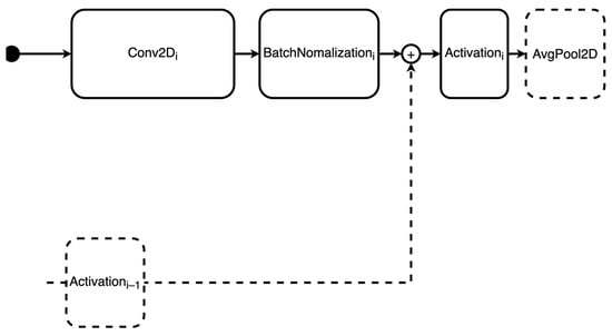
Figure 1.
Atomic block for type 1 neural topology.
The parameters used as search variables for type 1 neural topologies are listed in Table 2. Note that, as the convolution kernel is a square matrix, its size is a single integer number that accounts for both width and height.

Table 2.
Search variables for type 1 topologies.
The atomic block that defines type 2 topologies consists of a 2D convolution layer followed by an activation layer. Furthermore, the output of the activation goes through two parallel transformations: on one hand, it is fed into a batch normalization layer, on the other, it goes through a transposed 2D convolution, and the output is subtracted from the whole block’s input; after that, batch normalization is applied again, and the two parallel outputs are added together to form a single value. An additional max pooling layer may be applied to the block if it is the last one in the chain. The leading idea behind this structure was to generate a local error measure that would be added to the output of the single block and thus be considered by the subsequent block. The structure of type 2 atomic blocks is illustrated in Figure 2. Note that max pooling is applied after the final block in each type 2 topology.
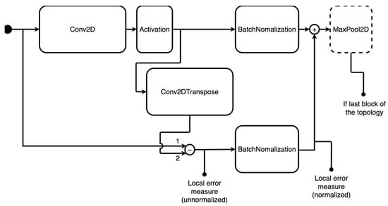
Figure 2.
Atomic block for type 2 neural topology. The numbers in the chart indicate the order for the subsequent subtraction operation.
The parameters that may vary between different type 2 topologies are almost the same as in Table 2. The sole exceptions are:
- Sum of residuals before activation layer: in this case, the topology does not include the possibility of summing the previous activation layer’s residual.
- Padding within the convolutional layers: for type 2 topologies, the ‘same’ padding is always applied.
4.2.2. Definition of the Search Strategy
The adopted search strategy follows the BO approach. For type 1 topologies, GP and RF surrogate models have been tested. In both cases, LCB was adopted as the acquisition function, with equal to 1.96 if the GP was the surrogate model and 1.5 if RF was used. It should also be noted that the RF surrogate was modeled over a uniform probability distribution instead of a normal one, as using the former showed better values in early experimentation stages.
4.2.3. Definition of the Performance Estimation Strategy
The reference feature set consisted of the vectors that had been extracted by an off-the-shelf pre-trained ResNet topology, from which the SoftMax layer used to perform classification was eliminated to make it a FE. This NN represents the standard benchmark for image classification, issued by MLCommons as part of the four Tiny benchmark case studies [47]. The reference FE configuration was kept identical to the standard ResNet, except for the aforementioned removal of the final SoftMax classification layer.
The performance of all topologies obtained by the searches was evaluated by computing the between the extracted feature sets and the reference feature sets. The reference FE was known to output high accuracy if attached to a SoftMax classifier, so the underlying assumption of this performance estimation strategy was that identical accuracy was expected if the topology obtained by the guided search produced identical features with respect to the reference.
Since the between two vectors with different dimensionalities cannot be computed, topologies that produced feature vectors with different dimensionalities were deemed invalid and were discarded. Furthermore, the BO search strategy verges towards the maximization of a function; as the target was to achieve the minimum possible, the metric was always multiplied by −1.
A flowchart describing the entirety of the experimental setup is presented in Figure 3.
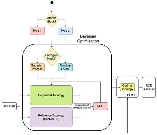
Figure 3.
Flowchart describing the experimental setup.
5. Results
Each configuration of the guided search was executed within the same testing environment, i.e., on the same computing machine and using identical virtual code environments. Experiments on the CIFAR-10 dataset were carried out for 48 h each, while those on the MNIST dataset were carried out for 4 h each. As Section 5.2 shows, a type 1 search space combined with an RF surrogate model proved to be the best performing configuration among the ones that were tried.
5.1. GP Surrogate Model with Type 1 Search Space
5.1.1. CIFAR-10 Dataset
The configuration that combined a GP surrogate model with type 1 topologies performed poorly. Over the span of roughly 9000 iterations, the search showed no signs of convergence towards a global optimum. This is very much visible in Figure 4, as the rolling average, which was computed every 10 iterations, stayed roughly constant over the whole search. Note that, as the invalid networks described in Section 4.2.3 were discarded, the line plot of the at each iteration is not continuous.
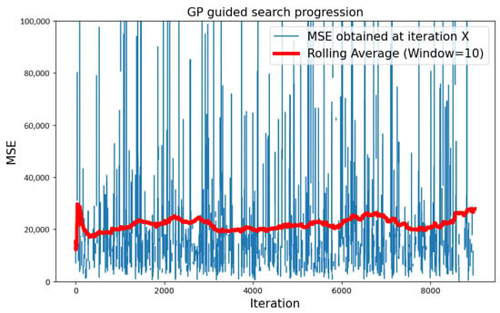
Figure 4.
Progression of the search over the CIFAR-10 dataset, with type 1 neural topology and GP surrogate model.
Figure 5 shows the variation in the optimum found by the algorithm over progressive iterations. After 48 h of execution, the best found was 216.128.
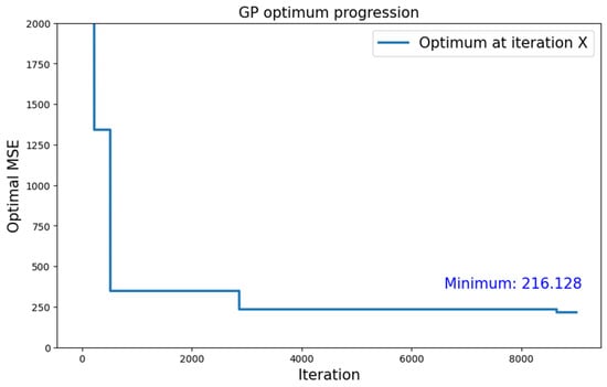
Figure 5.
Growth of the optimum over number of iterations for the search with type 1 neural topology and GP surrogate model applied to the CIFAR-10 dataset.
5.1.2. MNIST Dataset
Regarding the MNIST dataset, a similar behavior with respect to CIFAR-10 was observed. It is important to notice, though, that the best we found was lower by two orders of magnitude, equal to 2.537.
Figure 6 shows the progression of the search over a 4 h period. Since the time allotted for the execution of the experiment was significantly shorter, the sparsity of the line plot was more evident once the invalid values were discarded. Thus, circular indicators have been added to highlight the values we found.
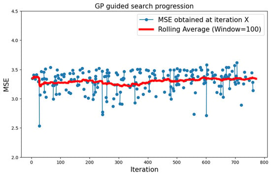
Figure 6.
Progression of the search over the MNIST dataset with type 1 neural topology and GP surrogate model.
Figure 7 shows the variation in the optimal found by the algorithm. Important progress can be seen in the initial iterations of the search. However, the minimum is reached very early, and progress stops in the subsequent iterations.
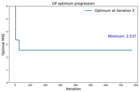
Figure 7.
Growth of the optimum over number of iterations for the search with type 1 neural topology and GP surrogate model applied to the MNIST dataset.
5.2. RF Surrogate Model with Type 1 Search Space
5.2.1. CIFAR-10 Dataset
The combination of type 1 topologies and an RF surrogate model proved to be the best performing configuration, as the best that it achieved was much lower than the ones obtained with the other two configurations. As Figure 8 shows, after 100 iterations of initial exploratory behavior, the rolling average showed almost constant growth and convergence towards values in the order of 10−1. In particular, the best we found was 0.640, as shown in Figure 9. Using RF as the surrogate model resulted in longer iterations, so the total number of attempted topologies was roughly six times lower with respect to the first configuration.
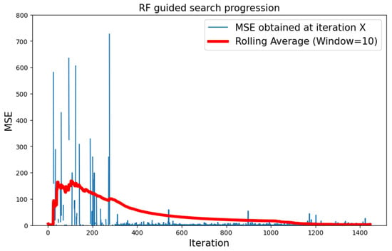
Figure 8.
Progression of the search with type 1 neural topology and RF surrogate model.
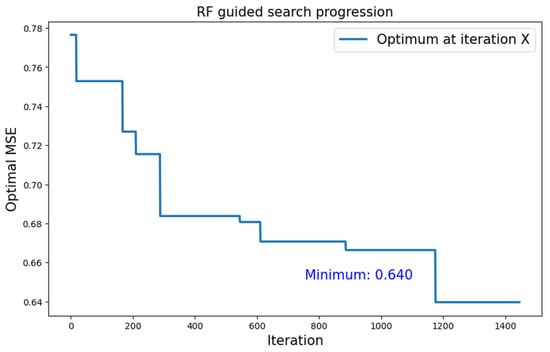
Figure 9.
Growth of the optimum found over the number of iterations for the search with type 1 neural topology and RF surrogate model.
The structure of the best performing topology for CIFAR-10 is illustrated in Figure 10. Its parameters are also listed in Table 3.

Figure 10.
Schema representing the best performing topology found in all searches for the CIFAR-10 dataset. Every group of three squares represents a block; the first square describes its kernel size, the second its number of filters and the third represents the presence/absence of regularization within the block. See Figure 1 for the composition of a singular block.

Table 3.
Variable settings for best found topology (CIFAR-10 dataset).
The best performing FE achieved by this search configuration still proved not to be enough for an accurate classification, as it scored 37.4% accuracy on the CIFAR-10 dataset once attached to a TinyRCE classifier [50]. TinyRCE had scored 78.5% accuracy when attached to the reference FE.
5.2.2. MNIST Dataset
While type 1 atomic blocks combined with an RF surrogate function worked best for what concerns CIFAR-10, they performed the worst when it comes to MNIST. In fact, the search progression shows little progress over time, as highlighted in Figure 11. Once again, circular indicators have been added to the line plot, for values to be more clearly visible.
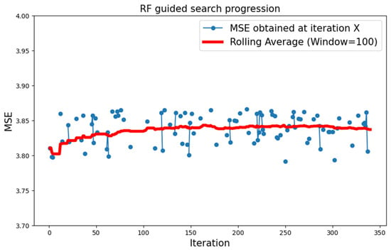
Figure 11.
Progression of the search over the MNIST dataset with type 1 neural topology and RF surrogate model.
Even though the progression of the search over time shows little progress, the optimal value was found rather late within this instance of the search, as shown by Figure 12. The optimal value that was found is equal to 3.778.
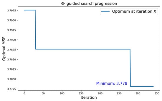
Figure 12.
Growth of the optimum over number of iterations for the search with type 1 neural topology and RF surrogate model applied to the MNIST dataset.
5.3. RF Surrogate Model with Type 2 Search Space
5.3.1. CIFAR-10 Dataset
Type 2 topologies combined with an RF surrogate model produced the worst results in terms of optimal . Although the behavior of the search showed similar trends with respect to the previous case, as shown by Figure 13, the average values were far worse than before, in the order of 105. The best performing network found by this search produced an of 8196.919, as shown in Figure 14.
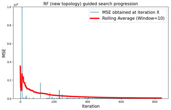
Figure 13.
Progression of the search with type 2 neural topology and RF surrogate model.
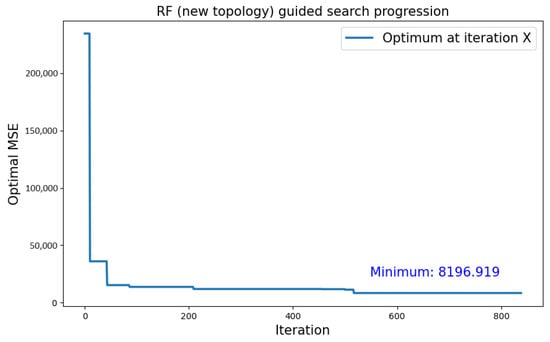
Figure 14.
Growth of the optimum over number of iterations for the search with type 2 neural topology and RF surrogate model.
5.3.2. MNIST Dataset
Type 2 neural blocks showed the most promise concerning when dealing with the MNIST dataset. As the search proceeded at a slower pace, less than 100 search iterations were completed within the allotted 4 h of execution. Nevertheless, the optimal value that was found within said time frame was the absolute lowest for MNIST: 1.468.
Figure 15 shows the progression of the search over time. Even though the rolling average line plot increases, being visibly affected by some outlier values, a slight but perceptible descent is hinted by the singular values themselves, once again highlighted with circular indicators for better visibility.
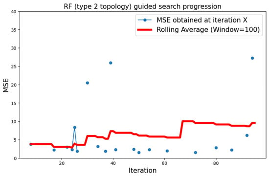
Figure 15.
Progression of the search over the MNIST dataset with type 2 neural topology and RF surrogate model.
Figure 16 shows the variation in the optimum found during the search.
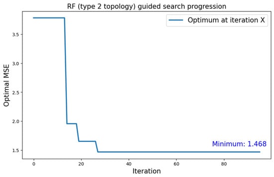
Figure 16.
Growth of the optimum over number of iterations for the search with type 2 neural topology and RF surrogate model applied to the MNIST dataset.
The structure of the best performing topology for the MNIST dataset is illustrated in Figure 17. Its parameters are also listed in Table 4. It is interesting to notice how a shallower, less complex FE proves to be more effective when dealing with the MNIST dataset compared to CIFAR-10 with respect to the search outcome. This difference between the two mirrors their composition, with CIFAR-10 being a more challenging dataset for NNs.
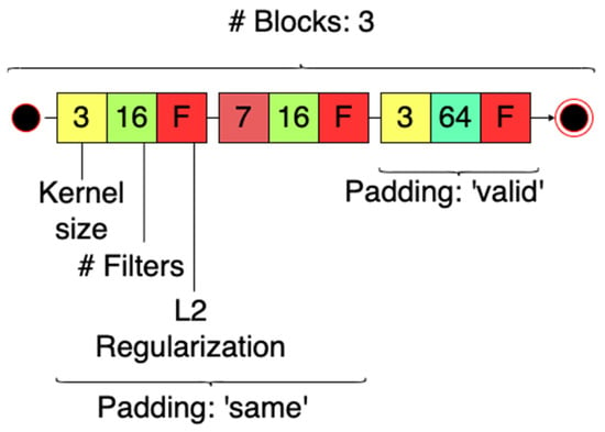
Figure 17.
Schema representing the best performing topology found in all searches for the MNIST dataset. Every group of three squares represents a block; the first square describes its kernel size, the second its number of filters and the third represents the presence/absence of regularization within the block. See Figure 2 for the composition of a singular block.

Table 4.
Variable settings for best found topology (MNIST dataset).
5.4. Summary of the Results
Table 5 summarizes the results obtained for all the experiments. The best results are highlighted in bold. It is evident that experiments on the MNIST dataset proved to be consistent in terms of magnitude, while the ones performed on CIFAR-10 have much more variable results. Nevertheless, the best absolute value was reached using type 1 neural blocks combined with an RF surrogate on the CIFAR-10 dataset, obtaining an optimal value below the targeted threshold of one.

Table 5.
Summary of obtained results. Best results for each dataset are highlighted in bold. Lower is better.
6. Discussion and Conclusions
This work proposed an approach to building an ELM CNN FE based on BO and NAS. Two search spaces were defined and tested, as well as two datasets and two different surrogate models. The output of each search iteration was an FE topology which was fed with image data, and an extracted set of feature vectors as the output. The datasets used were CIFAR-10 and MNIST. The output was then compared to a reference feature set, obtained by a trained FE based on the MLCommons Tiny benchmark ResNet model. The best result in terms of similarity to the reference feature set achieved an of 0.64 for the CIFAR-10 dataset, and 1.468 for the MNIST dataset. This outcome was still not enough to achieve a high classification accuracy using the FE as part of an ODL model; a TinyRCE classifier fed by the obtained features scored a 37.4% test set accuracy, 41.1% less than what the same classifier scored when fed with the reference features. Despite the unsatisfactory results collected so far, the experimental approach itself proposes an innovative integration of the NAS and BO techniques for the purpose of automatically designing a well-performing ELM FE, as well as a simple yet effective evaluation procedure that allows us to assess the quality of an FE without the necessity of training a learning agent connected to it. An automatically designed ELM FE becomes a fundamental building block for an NN to be deployed in ODL applications. Such an application would save all the memory required to store the activations and dataset needed to support backpropagation-based learning, which can eventually be reduced even further by weight selection techniques. This would lower the costs of inference workloads enough to satisfy what is required by ODL in tiny edge devices. Thus, the present study lays a solid groundwork for future improvements to the proposed approach. In conclusion, this work serves as an initializer and catalyst for future endeavors, inviting researchers to explore and build upon the theoretical framework presented herein. Future experimentation will focus on improving the search outcomes; in particular, the target to be achieved shall be lowered by at least one order of magnitude (10−2). The correlation between the achieved and the quality of the extracted features has not been studied enough; future investigations are required in this regard. Additionally, different metrics of feature quality could be experimented with. To improve the results of the search, new atomic block structures (e.g., based on attention layers, recurrent neural layers and many more) should be devised and tested, as well as different surrogate models and acquisition functions. Furthermore, the experimental approach should be tested on a greater variety of datasets, to better assess its generalizability. The datasets will include image recognition ones—e.g., CIFAR-100, MSCOCO14—and audio recognition ones such as Speech Commands.
Author Contributions
Conceptualization, A.P. and D.P.; methodology, A.P., D.P. and A.C.; software, A.P. and D.P.; validation, A.P., D.P. and A.C.; investigation, A.P. and D.P.; data curation, A.P.; writing—original draft preparation, A.P., D.P. and A.C.; writing—review and editing, A.P., D.P. and A.C.; visualization, A.P. and D.P.; supervision, D.P. and A.C.; project administration, D.P. All authors have read and agreed to the published version of the manuscript.
Funding
This research received no external funding.
Data Availability Statement
This research used publicly available data from [46]. The code used to perform the experiments is openly available for reproduction at the following link: www.github.com/andreapisa9/bayesian-elm-search/ (accessed on 30 December 2023).
Conflicts of Interest
The authors declare no conflicts of interest.
References
- Bianco, S.; Cadène, R.; Celona, L.; Napoletano, P. Benchmark Analysis of Representative Deep Neural Network Architectures. IEEE Access 2018, 6, 64270–64277. [Google Scholar] [CrossRef]
- Nagel, M.; Fournarakis, M.; Amjad, R.A.; Bondarenko, Y.; van Baalen, M.; Blankevoort, T. A White Paper on Neural Network Quantization. arXiv 2021, arXiv:2106.08295. [Google Scholar] [CrossRef]
- Li, H.; Kadav, A.; Durdanovic, I.; Samet, H.; Graf, H.P. Pruning Filters for Efficient ConvNets. arXiv 2016, arXiv:1608.08710. [Google Scholar] [CrossRef]
- Samie, F.; Bauer, L.; Henkel, J. From Cloud Down to Things: An Overview of Machine Learning in Internet of Things. IEEE Internet Things J. 2019, 6, 4921–4934. [Google Scholar] [CrossRef]
- Dhar, S.; Guo, J.; Liu, J.; Tripathi, S.; Kurup, U.; Shah, M. A Survey of On-Device Machine Learning: An Algorithms and Learning Theory Perspective. ACM Trans. Internet Things 2021, 2, 15. [Google Scholar] [CrossRef]
- O’Shea, K.; Nash, R. An Introduction to Convolutional Neural Networks. arXiv 2015, arXiv:1511.08458. [Google Scholar] [CrossRef]
- Cai, H.; Gan, C.; Zhu, L.; Han, S. TinyTL: Reduce Memory, Not Parameters for Efficient on-Device Learning. In Advances in Neural Information Processing Systems; Larochelle, H., Ranzato, M., Hadsell, R., Balcan, M.F., Lin, H., Eds.; Curran Associates, Inc.: Red Hook, NY, USA, 2020; Volume 33, pp. 11285–11297. [Google Scholar]
- Lin, J.; Zhu, L.; Chen, W.-M.; Wang, W.-C.; Gan, C.; Han, S. On-Device Training under 256kb Memory. arXiv 2022, arXiv:2206.15472. [Google Scholar]
- Huang, G.-B.; Zhu, Q.-Y.; Siew, C.K. Extreme Learning Machine: Theory and Applications. Neurocomputing 2006, 70, 489–501. [Google Scholar] [CrossRef]
- Wang, J.; Lu, S.; Wang, S.; Zhang, Y. A Review on Extreme Learning Machine. Multimed. Tools Appl. 2021, 81, 41611–41660. [Google Scholar] [CrossRef]
- Bull, D.R.; Zhang, F. Digital Picture Formats and Representations. In Intelligent Image and Video Compression; Elsevier: Amsterdam, The Netherlands, 2021; pp. 107–142. ISBN 978-0-12-820353-8. [Google Scholar]
- Bosse, S.; Maniry, D.; Wiegand, T.; Samek, W. A Deep Neural Network for Image Quality Assessment. In Proceedings of the 2016 IEEE International Conference on Image Processing (ICIP), Phoenix, AZ, USA, 25–28 September 2016; pp. 3773–3777. [Google Scholar]
- Ding, K.; Liu, Y.; Zou, X.; Wang, S.; Ma, K. Locally Adaptive Structure and Texture Similarity for Image Quality Assessment. In Proceedings of the 29th ACM International Conference on Multimedia, Virtual, 17 October 2021; pp. 2483–2491. [Google Scholar]
- Garnett, R. Bayesian Optimization; Cambridge University Press: Cambridge, UK; New York, NY, USA, 2023; ISBN 978-1-108-42578-0. [Google Scholar]
- Candelieri, A. A Gentle Introduction to Bayesian Optimization. In Proceedings of the 2021 Winter Simulation Conference (WSC), Phoenix, AZ, USA, 12 December 2021; pp. 1–16. [Google Scholar]
- Archetti, F.; Candelieri, A. Bayesian Optimization and Data Science; SpringerBriefs in Optimization; Springer International Publishing: Cham, Switzerland, 2019; ISBN 978-3-030-24493-4. [Google Scholar]
- Frazier, P.I. Bayesian Optimization. In Recent Advances in Optimization and Modeling of Contemporary Problems; Gel, E., Ntaimo, L., Shier, D., Greenberg, H.J., Eds.; INFORMS: Catonsville, MD, USA, 2018; pp. 255–278. ISBN 978-0-9906153-2-3. [Google Scholar]
- Guyon, I.; Sun-Hosoya, L.; Boullé, M.; Escalante, H.J.; Escalera, S.; Liu, Z.; Jajetic, D.; Ray, B.; Saeed, M.; Sebag, M.; et al. Analysis of the AutoML Challenge Series 2015–2018. In Automated Machine Learning; Springer: Berlin/Heidelberg, Germany, 2019. [Google Scholar]
- Perego, R.; Candelieri, A.; Archetti, F.; Pau, D. AutoTinyML for Microcontrollers: Dealing with Black-Box Deployability. Expert Syst. Appl. 2022, 207, 117876. [Google Scholar] [CrossRef]
- Močkus, J. On Bayesian Methods for Seeking the Extremum. In Optimization Techniques IFIP Technical Conference Novosibirsk, July 1–7, 1974; Marchuk, G.I., Ed.; Lecture Notes in Computer Science; Springer: Berlin/Heidelberg, Germany, 1975; Volume 27, pp. 400–404. ISBN 978-3-540-07165-5. [Google Scholar]
- Mockus, J. Bayesian Approach to Global Optimization: Theory and Applications; Mathematics and its applications, Soviet series; Kluwer Academic: Dordrecht, The Netherlands; Boston, MA, USA, 1989; ISBN 978-0-7923-0115-8. [Google Scholar]
- Berger, J.O. Statistical Decision Theory. In Time Series and Statistics; Eatwell, J., Milgate, M., Newman, P., Eds.; Palgrave Macmillan: London, UK, 1990; pp. 277–284. ISBN 978-0-333-49551-3. [Google Scholar]
- Breiman, L. Random Forests. Mach. Learn. 2001, 45, 5–32. [Google Scholar] [CrossRef]
- Hutter, F.; Hoos, H.H.; Leyton-Brown, K. Sequential Model-Based Optimization for General Algorithm Configuration. In Learning and Intelligent Optimization; Coello, C.A.C., Ed.; Lecture Notes in Computer Science; Springer: Berlin/Heidelberg, Germany, 2011; Volume 6683, pp. 507–523. ISBN 978-3-642-25565-6. [Google Scholar]
- Wang, X.; Jin, Y.; Schmitt, S.; Olhofer, M. Recent Advances in Bayesian Optimization. ACM Comput. Surv. 2023, 55, 287. [Google Scholar] [CrossRef]
- Wistuba, M.; Wistuba, M.; Rawat, A.; Pedapati, T. A Survey on Neural Architecture Search. arXiv 2019, arXiv:1905.01392. [Google Scholar]
- Van Son, D.; De Putter, F.; Vogel, S.; Corporaal, H. BOMP-NAS: Bayesian Optimization Mixed Precision NAS. In Proceedings of the 2023 Design, Automation & Test in Europe Conference & Exhibition (DATE), Antwerp, Belgium, 17–19 April 2023; pp. 1–2. [Google Scholar]
- White, C.; Neiswanger, W.; Savani, Y. BANANAS: Bayesian Optimization with Neural Architectures for Neural Architecture Search. Proc. AAAI Conf. Artif. Intell. 2021, 35, 10293–10301. [Google Scholar] [CrossRef]
- Shen, Y.; Li, Y.; Zheng, J.; Zhang, W.; Yao, P.; Li, J.; Yang, S.; Liu, J.; Cui, B. ProxyBO: Accelerating Neural Architecture Search via Bayesian Optimization with Zero-Cost Proxies. Proc. AAAI Conf. Artif. Intell. 2023, 37, 9792–9801. [Google Scholar] [CrossRef]
- Jiang, Y.; Yang, F.; Yu, B.; Zhou, D.; Zeng, X. Efficient Layout Hotspot Detection via Neural Architecture Search. ACM Trans. Des. Autom. Electron. Syst. 2022, 27, 62. [Google Scholar] [CrossRef]
- Yang, Z.; Zhang, S.; Li, R.; Li, C.; Wang, M.; Wang, D.; Zhang, M. Efficient Resource-Aware Convolutional Neural Architecture Search for Edge Computing with Pareto-Bayesian Optimization. Sensors 2021, 21, 444. [Google Scholar] [CrossRef]
- Elsken, T.; Metzen, J.H.; Hutter, F. Neural Architecture Search: A Survey. J. Mach. Learn. Res. 2019, 20, 1997–2017. [Google Scholar]
- Capogrosso, L.; Cunico, F.; Cheng, D.S.; Fummi, F.; Cristani, M. A Machine Learning-Oriented Survey on Tiny Machine Learning. arXiv 2023, arXiv:2309.11932. [Google Scholar] [CrossRef]
- Gong, Y.; Liu, L.; Yang, M.; Bourdev, L. Compressing Deep Convolutional Networks Using Vector Quantization. ArXiv Comput. Vis. Pattern Recognit. 2014, arXiv:1412.6115. [Google Scholar]
- Han, S.; Mao, H.; Dally, W.J. Deep Compression: Compressing Deep Neural Networks with Pruning, Trained Quantization and Huffman Coding. ArXiv Comput. Vis. Pattern Recognit. 2015, arXiv:1510.00149. [Google Scholar]
- Hinton, G.E.; Vinyals, O.; Dean, J. Distilling the Knowledge in a Neural Network. ArXiv Mach. Learn. 2015, arXiv:1503.02531. [Google Scholar]
- Cho, J.H.; Hariharan, B. On the Efficacy of Knowledge Distillation. In Proceedings of the IEEE/CVF International Conference on Computer Vision (ICCV), Seoul, Repulic of Korea, 27 October–2 November 2019. [Google Scholar]
- Deng, B.L.; Li, G.; Han, S.; Shi, L.; Xie, Y. Model Compression and Hardware Acceleration for Neural Networks: A Comprehensive Survey. Proc. IEEE 2020, 108, 485–532. [Google Scholar] [CrossRef]
- Ghimire, D.; Kil, D.; Kim, S. A Survey on Efficient Convolutional Neural Networks and Hardware Acceleration. Electronics 2022, 11, 945. [Google Scholar] [CrossRef]
- Lillicrap, T.P.; Santoro, A.; Marris, L.; Akerman, C.J.; Hinton, G. Backpropagation and the Brain. Nat. Rev. Neurosci. 2020, 21, 335–346. [Google Scholar] [CrossRef] [PubMed]
- Huang, G.-B.; Liang, N.-Y.; Liang, N.; Wong, P.K.; Rong, H.-J.; Saratchandran, P.; Sundararajan, N. On-Line Sequential Extreme Learning Machine. In Proceedings of the IASTED International Conference on Computational Intelligence, Calgary, AB, Canada, 4–6 July 2005; pp. 232–237. [Google Scholar]
- Huang, G.-B. Reply to “Comments on ‘The Extreme Learning Machine”. IEEE Trans. Neural Netw. 2008, 19, 1495–1496. [Google Scholar] [CrossRef]
- Huang, G.-B.; Zhou, H.; Ding, X.; Zhang, R.; Zhang, R. Extreme Learning Machine for Regression and Multiclass Classification. IEEE Trans. Syst. Man Cybern. Part B Cybern. 2012, 42, 513–529. [Google Scholar] [CrossRef] [PubMed]
- Cambria, E.; Huang, G.-B.; Kasun, L.L.C.; Zhou, H.; Vong, C.-M.; Lin, J.; Yin, J.; Cai, Z.; Liu, Q.; Li, K.; et al. Extreme Learning Machine. IEEE Intell. Syst. 2013, 28, 30–59. [Google Scholar] [CrossRef]
- Huang, G.-B. What Are Extreme Learning Machines? Filling the Gap between Frank Rosenblatt’s Dream and John von Neumann’s Puzzle. Cogn. Comput. 2015, 7, 263–278. [Google Scholar] [CrossRef]
- CIFAR-10 and CIFAR-100 Datasets. Available online: http://www.cs.toronto.edu/~kriz/cifar.html (accessed on 7 March 2023).
- Banbury, C.; Reddi, V.J.; Torelli, P.; Jeffries, N.; Kiraly, C.; Holleman, J.; Montino, P.; Kanter, D.; Warden, P.; Pau, D.; et al. MLPerf Tiny Benchmark. NeurIPS Datasets Benchmarks 2021, 1. Available online: https://datasets-benchmarks-proceedings.neurips.cc/paper_files/paper/2021/file/da4fb5c6e93e74d3df8527599fa62642-Paper-round1.pdf (accessed on 4 May 2023).
- LeCun, Y. The MNIST Database of Handwritten Digits. 1998. Available online: http://yann.lecun.com/exdb/mnist/ (accessed on 23 October 2023).
- He, K.; Zhang, X.; Ren, S.; Sun, J. Deep Residual Learning for Image Recognition. arXiv 2015, arXiv:1512.03385. [Google Scholar]
- Pau, D.P.; Pisani, A.; Aymone, F.M.; Ferrari, G. TinyRCE: Multipurpose Forward Learning for Resource Restricted Devices. IEEE Sens. Lett. 2023, 7, 5503104. [Google Scholar] [CrossRef]
Disclaimer/Publisher’s Note: The statements, opinions and data contained in all publications are solely those of the individual author(s) and contributor(s) and not of MDPI and/or the editor(s). MDPI and/or the editor(s) disclaim responsibility for any injury to people or property resulting from any ideas, methods, instructions or products referred to in the content. |
© 2024 by the authors. Licensee MDPI, Basel, Switzerland. This article is an open access article distributed under the terms and conditions of the Creative Commons Attribution (CC BY) license (https://creativecommons.org/licenses/by/4.0/).