Abstract
In this paper, a novel global optimization approach in the form of an adaptive hyper-heuristic, namely HyperDE, is proposed. As the naming suggests, the method is based on the Differential Evolution (DE) heuristic, which is a well-established optimization approach inspired by the theory of evolution. Additionally, two other similar approaches are introduced for comparison and validation, HyperSSA and HyperBES, based on Sparrow Search Algorithm (SSA) and Bald Eagle Search (BES), respectively. The method consists of a genetic algorithm that is adopted as a high-level online learning mechanism, in order to adjust the hyper-parameters and facilitate the collaboration of a homogeneous set of low-level heuristics with the intent of maximizing the performance of the search for global optima. Comparison with the heuristics that the proposed methodologies are based on, along with other state-of-the-art methods, is favorable.
1. Introduction
1.1. Problem
The problem under scrutiny is to find the global minimum of a function , with . Typically, the function has many variables and multiple local minima. The shape of the function is considered unknown, and we treat it as a black box; in particular, it is impossible to apply analytical methods in order to determine the minimum; also, the gradient is not available.
1.2. State of the Art
Currently, there are a plethora of approaches, namely heuristics, that are able to search the problem space for optimal solutions. An extensive list of heuristics can be found in [1]. We enumerate a few that are considered representative by being the most cited: Particle Swarm Optimization (PSO) [2], Simulated Annealing (SA) [3], Ant Colony Optimization (ACO) [4], Artificial Bee Colony (ABC) [5], Harmony Search (HS) [6], Gravitational Search Algorithm (GSA) [7], Firefly Algorithm (FA) [8]; many others have original traits. These methods intelligently evaluate the solution space, attempting to predict where the best solution is located, considering the past discovered solutions. A partial exploration is desired because the real world problems are complex; an exhaustive exploration is not feasible due to time and computational constraints. This being said, it is not guaranteed that the heuristic has found the global optima at the end of the search.
The stochastic methods that are considered in this paper are enumerated below.
Firstly, inspired by the theory of evolution, we have the basic Differential Evolution (DE) [9] algorithm along with two variants: the adaptive success-history based named SHADE [10] together with L-SHADE [11], which has additionally a linear population size reduction strategy.
Inspired by the behavior of groups of individuals found in nature, such as animals and insects, there are various swarm optimization algorithms: Sparrow Search Algorithm (SSA) [12], Bald Eagle Search (BES) [13], Whale Optimization Algorithm (WOA) [14], Harris Hawks Optimization (HHO) [15], and Hunger Games Search (HGS) [16]. The conceptual contribution and the underlying metaphor of some of these algorithms may be questionable [17], but many of them have good practical behavior.
Inspired by concepts from mathematics, we have Chaos Game Optimization (CGO) [18], while Slime Mold Algorithm (SMA) [19] can be considered a bio-inspired search algorithm.
Most of the techniques listed above are not far from the state-of-the-art; other methods are not so recent but are well established. What is to be taken into consideration is that DE together with SHADE and LSHADE are considered the key contenders in our methodology validation, the other algorithms being less relevant.
Each enumerated method performs in a different manner, excelling at solving a particular subset of problems while not being appropriate for solving some other problems. Many of the available heuristics have hyper-parameters whose values affect the performance of the search, therefore being able to tailor the algorithm to the given problem. It often happens that the methods fail to converge to the global optima, remaining stuck in a locally optimal solution instead and struggling to find a balance between exploration and exploitation.
Regarding the development of hyper-heuristics, the field of study is relatively new, with an increase in publications on this subject over the last three–four years [20]. There are several methods available, such as approaches based on genetic programming [21], graph-based [22], VNS-based [23], ant-based [24], tabu search-based [25], greedy selection-based [26], GA-based [27], simulated annealing-based [28], and reinforcement learning-based [29]. Those are several relevant examples that initiated the domain in various directions.
More recent hyper-heuristics that merit attention could be a simulated-annealing-based hyper-heuristic [30], a reinforcement learning-based hyper-heuristic [31], a genetic programming hyper-heuristic approach [32], a Bayesian-based hyper-heuristic approach [33] and a very appealing, highly general approach for continuous problems [34].
None of the above resembles our proposed method; as revealed in [20], most of the hyper-heuristics are designed to be applied in different domains, problems such as scheduling, timetabling, constraint satisfaction, routing policies, not continuous problems as in our study. Unlike our method, the existent high-level procedures are usually not population-based and do not make use of parallelization.
1.3. Our Contribution
Our plan is to define an adaptive hyper-heuristic [35] for adjusting the hyper-parameters of a set of low-level heuristics, in an online manner, such as to maximize the performance in finding the global minimum.
A hyper-heuristic is a methodology that automates the selection, generation and adaptation of lower level heuristics in order to solve difficult search problems. Therefore, instead of exploring the problem space directly, it explores the space of possible heuristics.
Accordingly, our proposed method has two optimization layers:
- The high-level adaptive algorithm, which is variant of the genetic algorithm (GA), is responsible for the process of online learning of the hyper-parameters of the basic heuristics.
- The low-level optimization algorithm can be any optimization method characterized by a set of hyper-parameters that are tuned by the high-level algorithm. The low-level algorithm acts through agents that directly attempt to solve the optimization problem by exploring the solution space.
After an analysis that consisted of the evaluation of various heuristics, DE was selected as the main low-level agent in the context of the proposed optimization method. The combination of our variant of GA at the high-level and DE at the low-level is called HyperDE. Two other algorithms, SSA and BES, were also considered appropriate to serve as agents. The resulting methods are called HyperSSA and HyperBES, respectively. The three methods are similar in approach, sharing the same high-level procedure, but differing by which algorithms are adopted as agents.
Each of the above optimization algorithms that are used as agents presents a set of hyper-parameters that influence the performance of their search. The most important in this paper, DE, has the following hyper-parameters: , weighting factor; , crossover rate; (integer), index of the mutation strategy (See Section 2 for details). In the HyperDE algorithm, a population of DE instances is managed by our GA, which tunes the triplets (F, CR, S) in the attempt to improve the search compared to the case where a single triplet of hyper-parameters is used.
By this endeavor, it is expected to obtain a methodology that is more general in its applicability, adapting without intervention to the given problem, resulting in a superior average performance given a set of problems without additional effort from the human agent. We consider it to be one possible approach to deal with the “No Free Lunch” theorem [36] successfully.
The evaluation and analysis of the proposed hyper-heuristics in comparison with the other enumerated algorithms was conducted on 12 benchmark functions provided by CEC 2022 competition. We show that HyperDE has indeed the best average performance and Friedman rank, followed by L-SHADE, while HyperSSA and HyperBES demonstrate to be significant improvements over their counterparts.
1.4. Content
In Section 2, the Differential Evolution algorithm is briefly presented, as it represents an important part of the proposed method; also, in Section 3, we recall the principles of the BES and SSA algorithms. In Section 4, a short description of the genetic algorithm can be found, which is the second key component of our method. In Section 5, we give a thorough presentation of the proposed methodology, containing also algorithms and diagrams. Finally, in Section 6, the results of the proposed method in comparison with some other algorithms are presented. Section 7 contains the conclusion of the paper.
2. Differential Evolution Algorithm Overview
Differential Evolution algorithm (DE) [9,37] is a population-based optimization method inspired by the theory of evolution. The algorithm starts from a set of solutions that are gradually improved by using operators such as selection, mutation and crossover. There are many variants of the algorithm; we concentrate on the ones that do not have self-adaptive capabilities or an external history, considering several mutation strategies that are of interest.
The DE basic structure is given in Algorithm 1. The population of NP vectors is initialized randomly and then improved in iterations. In each iteration, each individual can be replaced with a better one. A so-called donor vector is built with
where are individuals chosen randomly; they are distinct one from each other and from and F is a given weighting factor.
Then, a trial vector is produced by crossover from and the donor vector, with
where , , is a uniformly distributed random number generated for each j and is a random integer used to ensure that in all cases. The crossover rate dictates the probability with which the elements of the vector are changed with elements of the donor vector.
| Algorithm 1 Differential evolution algorithm |
| population size F ← weighting factor CR ← crossover probability Initialize randomly all individuals , t ← 0 while do for do Randomly choose , , from current population MUTATION: form the donor vector using the Formula (1) CROSSOVER: form trial vector with (2) EVALUATE: if , replace with trial vector end for t = t + 1 end while |
To the two hyper-parameters that influence the behavior of the method (F and CR), we add a third, the integer , representing the index of the mutation strategy. Among the many mutation operators that have been conceived and that can be an alternative to (1), in this paper we consider the following, singled out as “the six most widely used mutation schemes” in [37]:
- 0: “DE/rand/1” , which is (1)
- 1: “DE/best/1”
- 2: “DE/rand/2”
- 3: “DE/best/2”
- 4: “DE/current-to-best/1”
- 5: “DE/current-to-rand/1”
where the indexes , , , , are random integers that are all distinct, in the range , and different from i; they are generated for each mutant vector. represents the best individual from the current iteration.
Given the hyper-parameter or index S, the corresponding mutation strategy as defined above will be used by the DE agent, the algorithm remaining unchanged beyond that aspect. All the enumerated hyper-parameters will be manipulated by the genetic algorithm that will be presented.
3. Other Parameterized Heuristics
We briefly recall here information on two evolutionary algorithms that will be used, similarly with DE, as basic heuristics with which our hyper-heuristic works.
The Bald Eagle Search (BES) algorithm takes inspiration from the hunting behavior of bald eagles. The algorithm comprises three stages: selection of the search space, searching within the chosen space, and swooping.
In the selection stage, the eagles identify the best area within the search space where the maximum amount of food is available.
In the search stage, they scan the vicinity of the chosen space by spiraling and moving in various directions to look for prey.
During the swooping stage, the eagles move towards their target prey by shifting from their current best position. Overall, all points in the search space move towards the best point.
There are five hyper-parameters that need adjustment: (integer), determining the corner between point search in the central point; , determining the number of search cycles; , controlling the changes in position; and , increase the movement intensity of bald eagles towards the best and center points. Note that the above intervals are those recommended in the Python implementation from the library MEALPY [38] and we have used them. In the original work [13], the recommendations are , , , .
Sparrow search algorithm (SSA) [12] is a relatively new swarm optimization method inspired by the behavior of sparrows, specifically by the group wisdom, foraging and anti-predatory behaviors. There are two types of sparrows, producers and scroungers. The producers actively search for food while the scroungers exploit the producers by obtaining food from them. The roles are not fixed; an individual can shift from one foraging strategy to the other depending on its energy reserve. Each individual constantly tries to avoid being located at the periphery of the group to be less exposed to danger. Additionally, when one or more birds detect danger, they will chirp, the whole group flying away from the predator.
The hyper-parameters of SSA are , the alarm value; , the ratio of producers; , the ratio of sparrows who perceive the danger. Note that in [12], PD and SD are integers between 1 and n. We modify them in fractions of n in order to be able to optimize them more easily in the genetic algorithm.
4. Genetic Algorithm Overview
Genetic algorithm (GA) is a well established population-based optimization method inspired by the theory of evolution [39]. The approach is based on the Darwinian theory of survival of fittest in nature, adopting various biological-inspired operators such as crossover, mutation and fitness selection, operators that manipulate a set of chromosome representations. Algorithm 2 shows the basic GA structure.
| Algorithm 2 Genetic Algorithm |
while do Compute the fitness values of Compute the fitness values of end while return |
The algorithm starts by generating a random population of solutions . The solutions are evaluated via obtaining the corresponding fitnesses. Based on the fitnesses, a subset of the current population is selected as the parent population . The crossover operator is applied on the individuals from , obtaining a new set of solutions that may also mutate and are evaluated. At the end of the generation, the population of the next generation is obtained based on and . This process is repeated for a number of G iterations, resulting in , the final set of solutions to the problem.
In the HyperDE context, the chromosome associated with a DE instance is given by the hyper-parameters F, CR and S; for HyperSSA the genes are ST, PD and SD; while for HyperBES we have as genes of the chromosome a, , R, and . We denote as the number of hyper-parameters. The implementations of the basic GA operators are as follows. Single-point crossover was used, meaning that the first c values of the hyper-parameters (in the order given above) are taken from the first parent and the remaining from the second parent, where c is a random integer between 0 and the number of hyper-parameters. Mutation is implemented as the simple choice of a uniformly random real number (or integer, for S) in the interval of definition of each hyper-parameter. The fitness function will be described in the next section.
5. HyperDe Algorithm
As stated in Section 1.1, the goal is to find the minimum value of a function , with . The proposed hyper-heuristic, HyperDE, works like many other global optimization algorithms, by generating tentative solutions. The modality in which the solution space is explored gives the specific of a method.
In the two-layer structure mentioned in Section 1.3, HyperDE adopts as a high-level algorithm a form of steady-state Genetic Algorithm (GA). The (hyper-)population in this context is composed of various instances of DE, each with different hyper-parameters. Therefore, HyperDE orchestrates the collaboration and execution in parallel of the DE agents, manipulating the hyper-parameters and generated solutions.
The proposed method is an adaptive hyper-heuristic, where the genetic algorithm plays the role of an online learning mechanism, adjusting the hyper-parameters of the agent ensemble and adapting to the state of the problem while exploring the solution space. Thus, there is a learning process based on the performance shown in the past of each particular DE agent, exploring also the space of heuristics by the means of the standard GA operators: selection, crossover and mutation. Ergo, the optimization is accomplished on two levels, simultaneously, searching primarily the space of possible DE instances, but also the actual space of solutions to the given problem, as depicted in Figure 1.
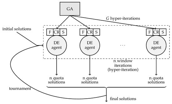
Figure 1.
Structure of the proposed adaptive hyper-heuristic approach.
The algorithm manages the hyper-population of DE agents, named , which is initialized with random values of the hyper-parameters F, CR, S. It also maintains a solution population , also initialized at random.
In order to evaluate the hyper-population , the DE agents are executed in parallel for a number of n_window iterations. Each agent is responsible for the generation of n_quota solutions; in other words, each DE agent has n_quota individuals. Therefore, the entire hyper-population explores the problem space in a parallel manner, obtaining at the end a set of solutions. The history set of solutions for agent g is denoted . The history consists of n_window sets of solutions, each corresponding to an iteration executed by agent g. represents the set of solutions obtained by agent g at the end of iteration i, and has the size = n_quota.
In order to assign a fitness to each agent of , the obtained histories of solutions are utilized in the procedure AgentsFitness (Algorithm 3). For each window iteration i, we compute the union of the agents solutions set in that particular iteration. The obtained union is sorted in ascending/descending order, depending on whether the problem to solve is one of minimization or maximization. Afterwards, a count is performed for each agent, counting how many of its solutions are found in the first third of the sorted union set, the count being then divided with for normalization. After the entire process, the average is computed over the entire window of iterations, thus obtaining the fitness value for each agent g.
| Algorithm 3 Computation of the fitness function for all agents |
| procedure AgentsFitness(, H, n_window) for each DE agent g in do end for for each iteration do for each DE agent g in do end for Sort in ascending/descending order by fitness the set for each DE agent g in do end for end for return end procedure |
The above-described operations are used in Algorithm 4, which updates the solution population and computes the fitness by calling Algorithm 3. For each agent, the current set of solutions is reduced firstly to half by random selection, after which the best n_quota solutions are retained. This set is the starting solution set for the agent in the next hyper-iteration, which consists of running the DE algorithm for n_window iterations. For the loop on the DE, agents can be executed in parallel. Finally, the procedure returns the union of the last sets of solutions of the entire ensemble of size , which is the new set of solutions , and also the set containing the fitnesses associated with the agents.
Algorithm 5 gathers the main operations. The evaluation procedure, as described above in Algorithm 4, which also explores the problem space with DE agents, is executed in each hyper-iteration. Based on the obtained HF fitnesses of the agents, the ensemble of the next hyper-iteration is computed. This is accomplished by firstly retaining the best half of the hyper-population of agents. Then, agents are randomly selected as parents in order to crossover and mutate (as described in Section 4), obtaining new agents; along with the elite of agents, they constitute the next hyper-generation. This process is sustained for G hyper-generations, or n_window DE iterations.
As explained, besides the fitnesses of the agents, the set of solutions is also updated, representing the union of all sets of solutions produced by each agent in the last iteration of the execution window; or simply, the solutions to the problem obtained at the end of hyper-iteration t.
| Algorithm 4 Evaluate and Explore algorithm |
procedure EvaluateAndExplore(, , n_quota, n_window) for each DE agent g in do solutions generated by the DE algorithm run for n_window iterations on population S end for AgentsFitness for each DE agent g in do end for return end procedure |
| Algorithm 5 HyperDE algorithm |
|
We note that the above algorithm has a high degree of generality. It is written for DE agents, which are characterized by three hyper-parameters. However, the algorithm can be adapted to any other global optimization heuristic, with any (nonzero) number of hyper-parameters.
As examples, we implemented the HyperSSA and HyperBES algorithms. The methods resemble the HyperDE hyper-heuristic in most regards, differing just by what type of agents are used. We have as agents the time instances of SSA heuristics in one case and instances of BES heuristics in the other case. Since the top-level procedure is highly decoupled from the agent’s inner workings, the algorithmic flows of the hyper-heuristics is the same as for HyperDE. We simply use the chromosomes presented in Section 3.
6. Results
The proposed adaptive hyper-heuristic methods are compared with 10 relatively new, state-of-the-art heuristics and well-established algorithms (including the basic heuristics that we employ: DE, BES, SSA), over a set of n_problems = 12 difficult problems, more exactly on the benchmarks provided by the CEC 2022 competition: (https://github.com/P-N-Suganthan/2022-SO-BO/blob/main/CEC2022%20TR.pdf, accessed on 18 September 2023). We have implemented our method in Python. The algorithms used for comparison, listed in Table 1 (to be later explained), have been taken from the MEALPY library [38] implementation in Python. Our programs can be found at https://github.com/mening12001/HyperHeuristica, accessed on 18 September 2023).

Table 1.
Errors of the evaluated methods on the CEC problems.
Our HyperDE hyper-heuristic is parameterized as follows: the number of hyper-iterations is , the evaluation window size is iterations, the hyper-population has size (the number of DE instances, or agents), where each agent has (the size of the solution population). In order for the comparison to be valid, the HyperDE hyper-heuristic along with the other methods should explore the same number of solutions. We note that HyperDE performs DE iterations and computes a population of solutions per iteration, resulting in a total of = 40,000 evaluated solutions. Therefore, the other methods will have as parameters: the number of iterations to be executed , and the size of population ; hence, the same volume of the solution space is explored at the end of execution. The other hyper-parameters specific to each method are set with default values, as recommended by the literature.
Each heuristic is evaluated by computing the relative error as described in Algorithm 6. The global minimum being known, the relative distance between the obtained result and the optimum is calculated.
For each problem, the heuristic in this case is evaluated n_tests = 60 times as described, averaging the relative error obtained in each evaluation. Finally, the average relative error obtained on each problem is aggregated again, obtaining the final relative error that reflects the overall performance of that algorithm (smaller is better).
| Algorithm 6 Evaluation, relative error |
for each problem in n_problems do for each test in n_tests do if then else end if end for end for |
As can be seen from Table 1, HyperDE has the minimal error on the selected suite of problems. We note also that HyperBES and HyperSSA perform better than their basic heuristics, BES and SSA.
Additionally, the Friedman ranking is computed, more precisely, the average rank over all the problems. The median was determined over the tests, for each problem and method. If, for a particular problem, the difference between the medians for two methods does not exceed , then the two methods have the same rank, which is the average of the corresponding ranks.
The results are given in Table 2 and show that HyperDE is the best from the entire suite of methods, at a significant distance from SHADE. Unlike in the error evaluation, SHADE is better then LSHADE. HyperBES preserves its fifth place, but HyperSSA falls down the ranking to tenth place, in particular below SSA.
Table 2.
Friedman ranking of the evaluated methods on the CEC problems.
One aspect that is consistent in both evaluations is that HyperDE proves to behave remarkably well relative to the other algorithms, it being conclusive that our hyper-heuristic is the best performer in the given context.
The execution times of the top performing algorithms are given in Table 3. They were measured on a MacBook Air computer with an M1 chip having a max CPU clock rate of 3.2 GHz and 8 GB memory. Note that the implementation of our methods is purely sequential and does not take advantage of the inherent parallelism of the agents; also, the implementation is plain and does not use any speeding-up trick. So, as expected, HyperDE is more time-consuming than the simpler methods such as SHADE and LSHADE, due to the additional computations and manipulations. HyperDE is roughly 60–80% slower. HyperSSA and HyperBES do not seem that efficient; this is because of the agents that are used, which are not as fast as DE.
Table 3.
Average times of the best methods (in minutes).
We reiterate that the number of function evaluations is the same for all methods; as long as the implementations are not fully optimized, this is the most important aspect in ensuring fairness of comparison. If the implementations would be equally well optimized for a specified computer, which is not an easy task, the results after a given time could be compared; even then, it may be argued that ideal conditions, like the inexistence of background processes, are nearly impossible to obtain. So, in these circumstances, we consider that our comparisons are reasonably fair.
The convergence of the top five methods on the entire suite of problems is illustrated in Figure 2 and Figure 3. The average over n_tests = 60 tests is shown, resulting in an average convergence curve, thus smoothing the stochastic behavior. The methods are executed for 200 iterations each, but only each fifth iteration is plotted in order to be aligned with the results of our hyper-heuristics, where the best result at the end of each hyper-iteration is shown.
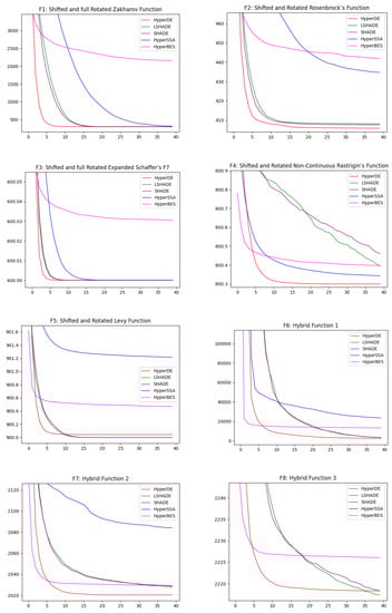
Figure 2.
Overall convergence of the best methods.
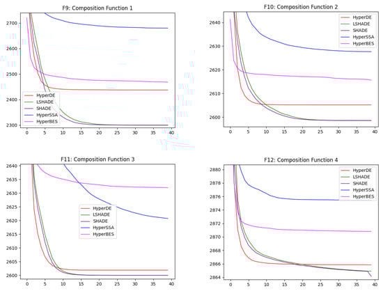
Figure 3.
Overall convergence of the best methods.
It is visible that HyperDE converges nearest to the global minimum on four functions: F2, F4, F6 and F7. For functions F1 and F3, HyperDE reaches about the same value as other methods, but it converges at the fastest rate. The convergence of HyperDE is more abrupt also on the other functions.
LSHADE and SHADE seem to take the lead on some of the other problems, not being drastically distant from our main method. HyperBES and HyperSSA are performing noticeably worse then the others. HyperBES is the most unimpressive on F1, F2, F3 and F11 while surpassing HyperSSA on F5, F6, F7, F8, F9, F10 and F12.
Box plots are shown in Figure 4, illustrating in more detail the distribution of the n_tests = 60 results of the algorithms. In most of the figures, the proposed method has a very reduced variance around the global optima, similarly to the other two DE variants. For F9, the variance is large while the median is aligned with the best result. In the F4 plot, HyperDE has the lowest median, followed by the other two proposed hyper-heuristics. However, HyperSSA and HyperBES perform worse on the other problems, with fairly large variance and a median quite far from the best solution, not being very clear which is the best of the two.
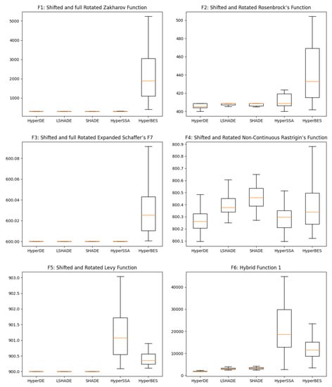
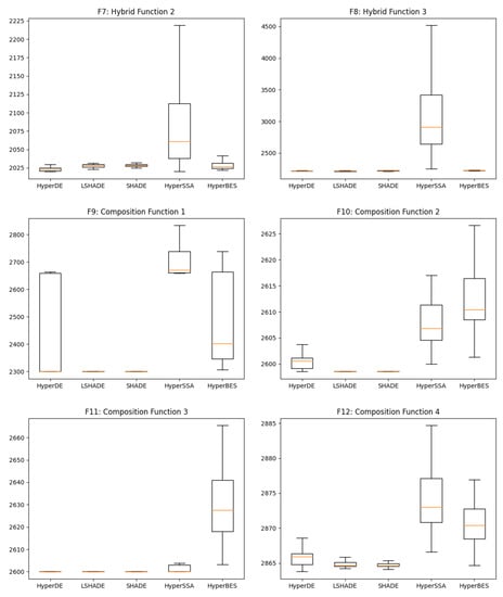
Figure 4.
Box plots of the best methods.
In Table 4, we can see a comparison of the performance of the proposed optimization method, HyperDE, with the other three methods from the DE family. The performance metrics include the best solution found (Best), the mean solution obtained (Mean), and the standard deviation (Std. Dev) of the solutions.
Table 4.
Method comparison for multiple problems.
As can be concluded, our method demonstrates an impressive performance, where it consistently outperforms the others in terms of the best solution. Regarding the mean, this is not always the case, as for F5, F8, F10, F11 and F12 the mean is slightly worse then for SHADE and LSHADE, while for F6 and F9 the inferiority is quite significant. Moreover, HyperDE achieves fairly low standard deviation values, indicating its reliability and ability to deliver stable and high-quality solutions.
Table 5 gives the results of the Wilcoxon signed-rank test. They show a statistically significant difference of HyperDE from the other methods on F1, as indicated by the extremely low p-values (approximately ). This is also the case for F2, F4, F6, and F7, exhibiting fairly low p-values in comparison with the other three methods, whereas on F10, F11, and F12, our methodology is surpassed by the other two self-adaptive algorithms. For F3, there is no significant difference between HyperDE and SHADE/LSHADE, the p-value being large, 0.16; however, DE is clearly worse than HyperDE. This situation is found for the other remaining problems (F5, F8, F9), where an actual winner cannot be proclaimed, except in comparison with the basic DE.
Table 5.
Results of Wilcoxon signed-rank test.
In summary, the results suggest that HyperDE consistently outperforms or shows comparable performance to the other optimization methods on most of the problems.
7. Conclusions
In this paper, a novel search methodology for global optimization was proposed in the form of an adaptive hyper-heuristic based on the Differential Evolution algorithm along with two other similar approaches. These approaches are highly general in their applicability, having a low number of hyper-parameters that need no adjustments. It was shown that the performance of the main algorithm, HyperDE, is superior relative to the other existent heuristics, obtaining a smaller relative error and the best Friedman rank on a benchmark from the CEC competition. The other two methods are not to be ignored, showing a significant improvement over their counterparts.
There are many possible directions of future work. We plan to improve the efficiency of our implementation, possibly by trying to take advantage of its inherent parallelism. Extension of our technique to other performant heuristic that use a small number of hyper-parameters is envisaged. Also, we plan to compare our method with other methods that tune the hyper-parameters.
Author Contributions
Conceptualization, A.-R.M.; methodology, A.-R.M. and B.D.; software, A.-R.M.; validation, A.-R.M. and B.D.; writing—original draft preparation, A.-R.M.; writing—review and editing, A.-R.M. and B.D.; visualization, A.-R.M.; supervision, B.D. All authors have read and agreed to the published version of the manuscript.
Funding
This work was supported in part by a grant of the Ministry of Research, Innovation and Digitization, CNCS-UEFISCDI, project number PN-III-P4-PCE-2021-0154, within PNCDI III.
Data Availability Statement
No new data were created or analyzed in this study.
Conflicts of Interest
The authors declare no conflict of interest.
References
- Ma, Z.; Wu, G.; Suganthan, P.N.; Song, A.; Luo, Q. Performance assessment and exhaustive listing of 500+ nature-inspired metaheuristic algorithms. Swarm Evol. Comput. 2023, 77, 101248. [Google Scholar] [CrossRef]
- Kennedy, J.; Eberhart, R. Particle swarm optimization. In Proceedings of the ICNN’95-International Conference on Neural Networks, Perth, WA, Australia, 27 November–1 December 1995; IEEE: New York, NY, USA, 1995; Volume 4, pp. 1942–1948. [Google Scholar]
- Kirkpatrick, S.; Gelatt, C.D., Jr.; Vecchi, M.P. Optimization by simulated annealing. Science 1983, 220, 671–680. [Google Scholar] [CrossRef]
- Dorigo, M.; Birattari, M.; Stutzle, T. Ant colony optimization. IEEE Comput. Intell. Mag. 2006, 1, 28–39. [Google Scholar] [CrossRef]
- Karaboga, D.; Basturk, B. A powerful and efficient algorithm for numerical function optimization: Artificial bee colony (ABC) algorithm. J. Glob. Optim. 2007, 39, 459–471. [Google Scholar] [CrossRef]
- Geem, Z.W.; Kim, J.H.; Loganathan, G.V. A new heuristic optimization algorithm: Harmony search. Simulation 2001, 76, 60–68. [Google Scholar] [CrossRef]
- Rashedi, E.; Nezamabadi-Pour, H.; Saryazdi, S. GSA: A gravitational search algorithm. Inf. Sci. 2009, 179, 2232–2248. [Google Scholar] [CrossRef]
- Yang, X.S. Firefly algorithms for multimodal optimization. In Proceedings of the International Symposium on Stochastic Algorithms, Sapporo, Japan, 26–28 October 2009; Springer: Berlin/Heidelberg, Germany, 2009; pp. 169–178. [Google Scholar]
- Storn, R.; Price, K. Differential evolution-a simple and efficient heuristic for global optimization over continuous spaces. J. Glob. Optim. 1997, 11, 341. [Google Scholar] [CrossRef]
- Tanabe, R.; Fukunaga, A. Success-history based parameter adaptation for differential evolution. In Proceedings of the 2013 IEEE Congress on Evolutionary Computation, Cancun, Mexico, 20–23 June 2013; IEEE: New York, NY, USA, 2013; pp. 71–78. [Google Scholar]
- Tanabe, R.; Fukunaga, A.S. Improving the search performance of SHADE using linear population size reduction. In Proceedings of the 2014 IEEE Congress on Evolutionary Computation (CEC), Beijing, China, 6–11 July 2014; IEEE: New York, NY, USA, 2014; pp. 1658–1665. [Google Scholar]
- Xue, J.; Shen, B. A novel swarm intelligence optimization approach: Sparrow search algorithm. Syst. Sci. Control Eng. 2020, 8, 22–34. [Google Scholar] [CrossRef]
- Alsattar, H.A.; Zaidan, A.; Zaidan, B. Novel meta-heuristic bald eagle search optimisation algorithm. Artif. Intell. Rev. 2020, 53, 2237–2264. [Google Scholar] [CrossRef]
- Mirjalili, S.; Lewis, A. The whale optimization algorithm. Adv. Eng. Softw. 2016, 95, 51–67. [Google Scholar] [CrossRef]
- Heidari, A.A.; Mirjalili, S.; Faris, H.; Aljarah, I.; Mafarja, M.; Chen, H. Harris hawks optimization: Algorithm and applications. Future Gener. Comput. Syst. 2019, 97, 849–872. [Google Scholar] [CrossRef]
- Yang, Y.; Chen, H.; Heidari, A.A.; Gandomi, A.H. Hunger games search: Visions, conception, implementation, deep analysis, perspectives, and towards performance shifts. Expert Syst. Appl. 2021, 177, 114864. [Google Scholar] [CrossRef]
- Camacho-Villalón, C.L.; Dorigo, M.; Stützle, T. Exposing the grey wolf, moth-flame, whale, firefly, bat, and antlion algorithms: Six misleading optimization techniques inspired by bestial metaphors. Int. Trans. Oper. Res. 2023, 30, 2945–2971. [Google Scholar] [CrossRef]
- Talatahari, S.; Azizi, M. Chaos Game Optimization: A novel metaheuristic algorithm. Artif. Intell. Rev. 2021, 54, 917–1004. [Google Scholar] [CrossRef]
- Li, S.; Chen, H.; Wang, M.; Heidari, A.A.; Mirjalili, S. Slime mould algorithm: A new method for stochastic optimization. Future Gener. Comput. Syst. 2020, 111, 300–323. [Google Scholar] [CrossRef]
- Gárate-Escamilla, A.K.; Amaya, I.; Cruz-Duarte, J.M.; Terashima-Marín, H.; Ortiz-Bayliss, J.C. Identifying Hyper-Heuristic Trends through a Text Mining Approach on the Current Literature. Appl. Sci. 2022, 12, 10576. [Google Scholar] [CrossRef]
- Burke, E.K.; Hyde, M.R.; Kendall, G.; Ochoa, G.; Ozcan, E.; Woodward, J.R. Exploring hyper-heuristic methodologies with genetic programming. In Computational Intelligence; Springer: Berlin/Heidelberg, Germany, 2009; pp. 177–201. [Google Scholar]
- Burke, E.K.; McCollum, B.; Meisels, A.; Petrovic, S.; Qu, R. A graph-based hyper-heuristic for educational timetabling problems. Eur. J. Oper. Res. 2007, 176, 177–192. [Google Scholar] [CrossRef]
- Hsiao, P.C.; Chiang, T.C.; Fu, L.C. A vns-based hyper-heuristic with adaptive computational budget of local search. In Proceedings of the 2012 IEEE Congress on Evolutionary Computation, Brisbane, Australia, 10–15 June 2012; IEEE: New York, NY, USA, 2012; pp. 1–8. [Google Scholar]
- Chen, P.C.; Kendall, G.; Berghe, G.V. An ant based hyper-heuristic for the travelling tournament problem. In Proceedings of the 2007 IEEE Symposium on Computational Intelligence in Scheduling, Honolulu, Hawaii, 1–5 April 2007; IEEE: New York, NY, USA, 2007; pp. 19–26. [Google Scholar]
- Burke, E.K.; Kendall, G.; Soubeiga, E. A tabu-search hyperheuristic for timetabling and rostering. J. Heuristics 2003, 9, 451–470. [Google Scholar] [CrossRef]
- Cowling, P.I.; Chakhlevitch, K. Using a large set of low level heuristics in a hyperheuristic approach to personnel scheduling. In Evolutionary Scheduling; Springer: Berlin/Heidelberg, Germany, 2007; pp. 543–576. [Google Scholar]
- Han, L.; Kendall, G. Guided operators for a hyper-heuristic genetic algorithm. In Proceedings of the Australasian Joint Conference on Artificial Intelligence, Perth, Australia, 3–5 December 2003; Springer: Berlin/Heidelberg, Germany, 2003; pp. 807–820. [Google Scholar]
- Bai, R.; Kendall, G. An investigation of automated planograms using a simulated annealing based hyper-heuristic. In Metaheuristics: Progress as Real Problem Solvers; Springer: Berlin/Heidelberg, Germany, 2005; pp. 87–108. [Google Scholar]
- Resende, M.G.; de Sousa, J.P.; Nareyek, A. Choosing search heuristics by non-stationary reinforcement learning. In Metaheuristics: Computer Decision-Making; Springer: Berlin/Heidelberg, Germany, 2004; pp. 523–544. [Google Scholar]
- Lim, K.C.W.; Wong, L.P.; Chin, J.F. Simulated-annealing-based hyper-heuristic for flexible job-shop scheduling. In Engineering Optimization; Taylor & Francis: Abingdon, UK, 2022; pp. 1–17. [Google Scholar]
- Qin, W.; Zhuang, Z.; Huang, Z.; Huang, H. A novel reinforcement learning-based hyper-heuristic for heterogeneous vehicle routing problem. Comput. Ind. Eng. 2021, 156, 107252. [Google Scholar] [CrossRef]
- Lin, J.; Zhu, L.; Gao, K. A genetic programming hyper-heuristic approach for the multi-skill resource constrained project scheduling problem. Expert Syst. Appl. 2020, 140, 112915. [Google Scholar] [CrossRef]
- Oliva, D.; Martins, M.S. A Bayesian based Hyper-Heuristic approach for global optimization. In Proceedings of the 2019 IEEE Congress on Evolutionary Computation (CEC), Wellington, New Zealand, 10–13 June 2019; IEEE: New York, NY, USA, 2019; pp. 1766–1773. [Google Scholar]
- Cruz-Duarte, J.M.; Amaya, I.; Ortiz-Bayliss, J.C.; Conant-Pablos, S.E.; Terashima-Marín, H.; Shi, Y. Hyper-heuristics to customise metaheuristics for continuous optimisation. Swarm Evol. Comput. 2021, 66, 100935. [Google Scholar] [CrossRef]
- Burke, E.K.; Hyde, M.R.; Kendall, G.; Ochoa, G.; Özcan, E.; Woodward, J.R. A classification of hyper-heuristic approaches: Revisited. In Handbook of Metaheuristics; Springer: Berlin/Heidelberg, Germany, 2019; pp. 453–477. [Google Scholar]
- Adam, S.P.; Alexandropoulos, S.A.N.; Pardalos, P.M.; Vrahatis, M.N. No free lunch theorem: A review. In Approximation and Optimization: Algorithms, Complexity and Applications; Springer: Berlin/Heidelberg, Germany, 2019; pp. 57–82. [Google Scholar]
- Georgioudakis, M.; Plevris, V. A comparative study of differential evolution variants in constrained structural optimization. Front. Built Environ. 2020, 6, 102. [Google Scholar] [CrossRef]
- Thieu, N.V.; Mirjalili, S. MEALPY: A Framework of The State-of-The-Art Meta-Heuristic Algorithms in Python. 2022. Available online: https://zenodo.org/record/6684223 (accessed on 18 September 2023).
- Katoch, S.; Chauhan, S.S.; Kumar, V. A review on genetic algorithm: Past, present, and future. Multimed. Tools Appl. 2021, 80, 8091–8126. [Google Scholar] [CrossRef] [PubMed]
Disclaimer/Publisher’s Note: The statements, opinions and data contained in all publications are solely those of the individual author(s) and contributor(s) and not of MDPI and/or the editor(s). MDPI and/or the editor(s) disclaim responsibility for any injury to people or property resulting from any ideas, methods, instructions or products referred to in the content. |
© 2023 by the authors. Licensee MDPI, Basel, Switzerland. This article is an open access article distributed under the terms and conditions of the Creative Commons Attribution (CC BY) license (https://creativecommons.org/licenses/by/4.0/).