Intelligent Identification of Trend Components in Singular Spectrum Analysis

Abstract

Singular spectrum analysis (SSA) is a non-parametric adaptive technique used for time series analysis. It allows solving various problems related to time series without the need to define a model. In this study, we focus on the problem of trend extraction. To extract trends using SSA, a grouping of elementary components is required. However, automating this process is challenging due to the nonparametric nature of SSA. Although there are some known approaches to automated grouping in SSA, they do not work well when the signal components are mixed. In this paper, a novel approach that combines automated identification of trend components with separability improvement is proposed. We also consider a new method called EOSSA for separability improvement, along with other known methods. The automated modifications are numerically compared and applied to real-life time series. The proposed approach demonstrated its advantage in extracting trends when dealing with mixed signal components. The separability-improving method EOSSA proved to be the most accurate when the signal rank is properly detected or slightly exceeded. The automated SSA was very successfully applied to US Unemployment data to separate an annual trend from seasonal effects. The proposed approach has shown its capability to automatically extract trends without the need to determine their parametric form.

1. Introduction

Singular spectrum analysis (SSA) [1,2,3,4] is a non-parametric, adaptive technique used for time series analysis. It can effectively solve various problems, such as decomposing a time series into identifiable components (e.g., trends, periodicities, and noise). Trend extraction is especially useful in its own right, as well as a prerequisite for forecasting. The benefit of SSA over other methods is that it does not require that the time series and its components assume any specific parametric form. Nevertheless, automation of SSA has yet to be achieved, limiting its application. This paper presents a step in the direction of automating SSA for trend extraction.

SSA consists of two stages: Decomposition and Reconstruction. After the Decomposition step, it is necessary to group the obtained elementary components in order to reconstruct time series components, such as the trend. However, automating the grouping step in SSA is challenging due to the nonparametric nature of SSA. The success of grouping depends on the separability of the component of interest, meaning that there should be no mixture of elementary components corresponding to the trend with elementary components corresponding to the residual (periodicity or noise).

Novelty. While there are some known algorithms for automated grouping [5,6,7,8], they only work if signal components such as trend and periodic ones are separable with SSA. However, if trend and periodic components are mixed, automated grouping is not able to separate them and, as a consequence, cannot extract the trend. At the same time, there are algorithms that can improve separability [9]. This paper proposes a novel approach to automated trend extraction that combines automated trend identification and separability improvement with automation of the methods of separability improvement called IOSSA, FOSSA and EOSSA (OSSA means Oblique SSA). The latter algorithm is new and was not justified before; therefore, we include a separate section devoted to EOSSA.

To connect the paper’s structure with the proposed method, we present a flowchart in Figure 1.

Paper’s structure. Let us outline the structure of this paper. Section 2 (the green block in Figure 1) provides a brief description of the SSA algorithm and the basic concepts. Section 3 (the blue block in Figure 1) introduces the notion of separability and briefly describes the methods for improving separability. In Section 4 (the yellow blocks in Figure 1), the method for automated identification of trends is described, followed by the proposal of combined methods that can both improve the separability of the trend components and automatically extract them. Section 5 (the violet block in Figure 1) is dedicated to justifying the EOSSA method, which was introduced in Section 3. The proposed methods are compared through numerical experiments, and their results are demonstrated for a real-life time series in Section 6. Section 7 concludes the paper.

2. SSA Algorithm and Linear Recurrence Relations

A comprehensive description of the SSA algorithm and its theory can be found in [4]. In Algorithm 1, we present a specific case for extracting the trend.

Consider a time series ${\mathsf{X}}_N=(x_1,\dots ,x_N)$ of length N, where $x_n\in \mathbb{R}$.

Algorithm 1 Basic SSA for trend extraction.

Parameters: window length L, $1<L<N$, and method of identifying trend components. Construction of trajectory matrix: $\mathbf{X}=\mathcal{T}\left(\mathsf{X}\right)=[X_1:\dots :X_K]$ is a Hankel matrix, where $X_i={(x_i,\dots ,x_{i+L-1})}^{\mathrm{T}}$, $1\le i\le K$, $K=N-L+1$. The SVD of the trajectory matrix: $\mathbf{X}={\displaystyle \sum _{i=1}^d}\sqrt{{\lambda }_i}{U}_i{V}_i^{\mathrm{T}}={\displaystyle \sum _{i=1}^d}{\mathbf{X}}_i$, $d=\mathrm{rank}\mathbf{X}$. Here ${\mathbf{X}}_i$, $i=1,\dots ,d$, are the elementary matrices of rank 1. Identification of trend components of the SVD using the given method of identifying trend components: identification of slowly varying elementary time series ${\tilde{\mathsf{X}}}_i={\mathcal{T}}^{-1}\left({\mathsf{\Pi }}_{\mathcal{H}}\left({\mathbf{X}}_i\right)\right)$, where ${\mathsf{\Pi }}_{\mathcal{H}}$ is the hankelization operator. Denote by $I=\{i_1,\dots ,i_t\}$ the set of slowly varying components. Estimation of trend $\tilde{\mathsf{X}}={\sum }_{i\in I}{\tilde{\mathsf{X}}}_i$.

By definition, the L-rank of a time series is equal to the rank of its L-trajectory matrix r. It turns out that for L such that $min(L,K)>r$ (assuming that the time series is long enough and such window lengths exist), the L-rank of the time series does not depend on L and is called simply the rank of the time series. Further reasoning will require knowledge of the ranks of particular time series. From [4] we know that the rank of a sinusoid with frequency $\omega$, $0<\omega <0.5$, is 2, and the rank of an exponential series and a sinusoid with period two equals 1. The same is valid for exponentially-modulated sinusoids. The rank of a polynomial series of degree ℓ equals $\ell +1$.

An infinite series $\mathsf{S}$ is a time series of rank r if and only if it is governed by a linear recurrence relation (LRR) of order r, i.e., $s_{n+r}={\sum }_{i=1}^r{a}_i{s}_{n+r-i}$, $a_i\ne 0$, and this LRR is minimal. The minimal LRR is the only one, but obviously, there are many LRRs of higher order. If r exists, we call such signals time series of finite rank; overwise, we refer to them as time series of infinite rank.

A characteristic polynomial of the form $P\left(\mu \right)={\mu }^r-{\sum }_{i=1}^r{a}_i{\mu }^{r-i}$ is associated with the LRR. Let it have k complex roots ${\mu }_1,\dots ,{\mu }_k$, which are called signal roots, and ${\mu }_i$ have multiplicity $m_i$, ${\sum }_{i=1}^k{m}_i=r$.

Through these roots, we can express the general parametric form of the time series [10] (Theorem 3.1.1)

$$s_n=\sum _{i=1}^k{P}_{m_i}\left(n\right){\mu }_i^n,$$

(1)

where $P_m\left(n\right)$ denotes a polynomial of degree m in n.

The decomposition of a time series into components of a certain structure using SSA, as well as their prediction, does not require knowledge of the explicit form of the time series (1), which greatly expands the applicability of SSA. However, if the signal fits this model, there is a method that allows one to estimate the non-linear parameters entering the time series, namely, ${\mu }_i$; this is the ESPRIT method [11] (another name of ESPRIT for time series is HSVD [12]). For instance, let the trend correspond to the leading r components in the SVD decomposition of the trajectory matrix of the time series. Let $\mathbf{P}=[U_1:\dots :U_r]$, and $\underline{\mathbf{P}}$ and $\overline{\mathbf{P}}$ be the matrices obtained by removing the last and first rows of a matrix $\mathbf{P}$, respectively. Then the estimates of single roots ${\mu }_i$, $i=1,\dots ,r$, will be the eigenvalues of the matrix ${\underline{\mathbf{P}}}^{†}\overline{\mathbf{P}}$ (LS-ESPRIT). In the case of a root of multiplicity larger than 1, when numerical methods are employed, the result of estimation will be a group of close roots, with a size equal to the multiplicity of the root.

In the real case, denoting ${\mu }_i={\rho }_i{e}^{2\pi {\omega }_i\mathsf{i}}$, we obtain an explicit form of the time series as a sum of polynomials multiplied by exponentially-modulated harmonics:

$$s_n=\sum _{i=1}^k{P}_{m_i}\left(n\right){\rho }_i^{n}cos(2\pi {\omega }_{i}n+{\varphi }_i);$$

ESPRIT estimates the parameters ${\rho }_i$ and ${\omega }_i$. In what follows we will consider the real case.

3. Separability Improvement

3.1. Separability of Time Series Components

For the proper decomposition of a time series into a sum of components, these components must be separable. By separability we mean the following. Let the time series be a sum of two components in which we are interested separately. If the decomposition of the entire time series into elementary components can be divided into two parts, with one part referring to the first component and the other part referring to the second component, then by gathering these components into groups and summing them up, we will obtain exactly the components we are interested in, that is, to separate them. If the decomposition into elementary components is not unique (which is the case with singular value decomposition), then the notions of weak and strong separability arise. Weak separability is defined as the existence of a decomposition in which the components of the time series are separable. Strong separability means the separability of the components in any decomposition provided by the decomposition method in use. Therefore, the main goal in obtaining a decomposition of a time series is to achieve strong separability.

Without loss of generality, let us formalize this notion for the sum of two time series, following [4] (Section 1.5 and Chapter 6). Let $\mathsf{X}={\mathsf{X}}_1+{\mathsf{X}}_2$ be a time series of length N, the window length L be chosen and the time series ${\mathsf{X}}_1$ and ${\mathsf{X}}_2$ correspond to the trajectory matrices ${\mathbf{X}}_1$ and ${\mathbf{X}}_2$. The SVDs of the trajectory matrices are ${\mathbf{X}}_1={\sum }_{i=1}^{r_1}\sqrt{{\lambda }_{1i}}{U}_{1i}{V}_{1i}^{\mathrm{T}}$ and ${\mathbf{X}}_2={\sum }_{j=1}^{r_2}\sqrt{{\lambda }_{2j}}{U}_{2j}{V}_{2j}^{\mathrm{T}}$. Then

• Time series ${\mathsf{X}}_1$ and ${\mathsf{X}}_2$ are weakly separable using SSA, if ${\mathbf{X}}_1{\mathbf{X}}_2^{\mathrm{T}}={\mathbf{0}}_{L,L}$ and ${\mathbf{X}}_1^{\mathrm{T}}{\mathbf{X}}_2={\mathbf{0}}_{K,K}$.
• Weakly separable time series ${\mathsf{X}}_1$ and ${\mathsf{X}}_2$ are strongly separable, if ${\lambda }_{1i}\ne {\lambda }_{2j}$ for each $i=1,\dots ,r_1$ and $j=1,\dots ,r_2$.

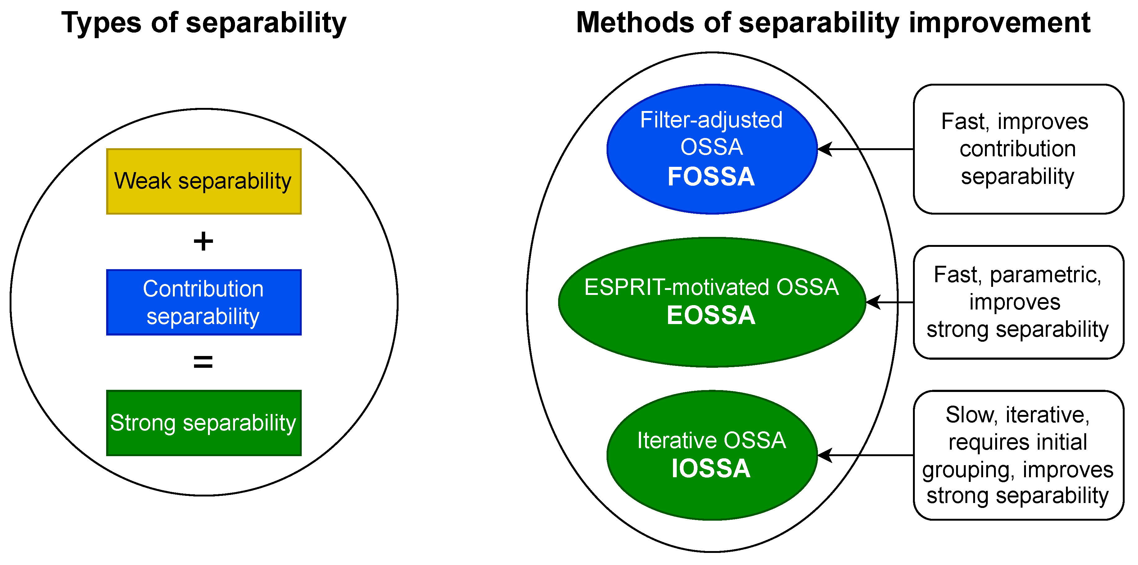
Thus, strong separability consists of weak separability, which is related to the orthogonality of the time series components (more precisely, orthogonality of their L- and K-lagged vectors), and of different contributions of these components (that is, different contributions of elementary components produced by them). We will call the latter contribution separability. The conclusion of this is that to improve weak separability one needs to adjust the notion of orthogonality of the time series components, and to improve contribution separability, one needs to change the contributions of the components. To obtain strong separability, both weak and contribution separabilities are necessary.

3.2. Methods of Separability Improvement

The following methods are used to improve separability: FOSSA [9], IOSSA [9]. and EOSSA. Algorithms and implementations of the FOSSA and IOSSA methods can be found in [13,14]. A separate Section 5 is devoted to EOSSA. The common part of the methods’ names is OSSA, which stands for Oblique SSA.

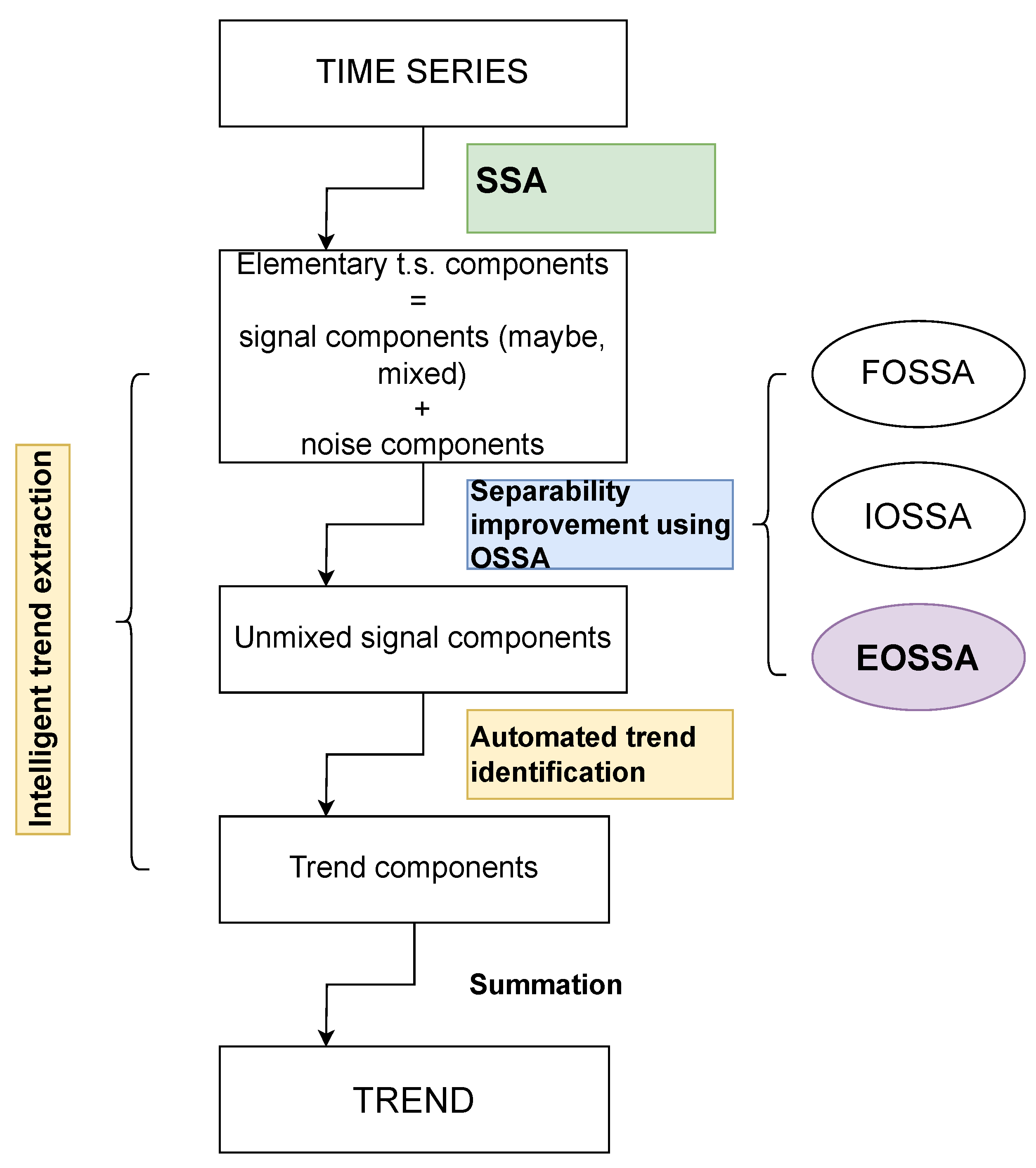
All methods are nested (that is, they are add-ons to the SVD step of Algorithm 1) and satisfy the following scheme.

Scheme of applying nested methods:

• Perform the SVD step of Algorithm 1.
• Select t of the SVD components, presumably related to the signal; denote their sum $\mathbf{Y}$.
• Perform re-decomposition of $\mathbf{Y}$ by one of nested methods to improve the separability of the signal components (nested decomposition).

In all algorithms for improving separability, we first select the components of the expansion to be improved. Consider the case where the leading t components are selected. The algorithms’ input is a matrix $\mathbf{Y}$ of rank t, recovered from the leading t components, not necessarily Hankel. Denote $\mathsf{Y}={\mathcal{T}}^{-1}\circ {\mathsf{\Pi }}_{\mathcal{H}}\left(\mathbf{Y}\right)$. Then the result of the algorithms is the decomposition of the matrix $\mathbf{Y}$ and of the time series $\mathsf{Y}$ generated by $\mathbf{Y}$.

Figure 2 illustrates the relationship between the various methods of improving separability and the different types of separability, which are indicated by color. The characteristics of these methods are briefly listed. In the following paragraphs, we provide a more detailed description of each method.

The Filter-adjusted Oblique SSA (FOSSA) [9] method is easy to use; however, it can improve only contribution separability, that is, strong separability if the weak separability holds. The idea behind a variation of the method, called DerivSSA (this is the one we will use in this work), is to use the time series derivative (going to consecutive differences in the discrete case) that changes the component contributions. The method calculates $\Phi \left(\mathbf{Y}\right)=[Y_2-Y_1:\cdots :Y_K-Y_{K-1}]$, whose column space belongs to the column space of $\mathbf{Y}$, and then constructs the SVD of the matrix $\mathbf{Z}=[\mathbf{Y}:\gamma \Phi (\mathbf{Y}\left)\right]$, $\gamma >0$. The [14] (Algorithm 2.11) provides an extended version of the algorithm that makes different contributions of the components to the time series, regardless of whether those contributions were the same or different. It is implemented in [13] and that is what we will use. We will take the default value of $\gamma$, so we will not specify it in the algorithm parameters. Thus, the only parameter of the algorithm is t. We will write FOSSA(t).

The Iterative Oblique SSA (IOSSA) [9] method can improve weak separability. It can also improve the strong separability, but the use of IOSSA is quite time-consuming, so when there is weak separability, it does not make sense to use it. The idea behind the method is to change the standard Euclidean inner product $(X,Y)=X^{\mathrm{T}}Y$ to the oblique inner product ${(X,Y)}_{\mathbf{A}}=X^{\mathrm{T}}\mathbf{A}Y$ for a symmetric positive semi-definite matrix $\mathbf{A}$. This approach allows any two non-collinear vectors to become orthogonal. It is shown in [9] that any two sufficiently long time series governed by LRRs can be made exactly separable by choosing suitable inner products in the column and row signal spaces. The algorithm uses iterations, starting from the standard inner product, to find the appropriate matrices that specify the inner products. The detailed algorithm is given in [14]. We will use the implementation from [13]. The parameter of the algorithm is the initial grouping $\{1,\dots ,t\}={⨆}_{j=1}^k{I}_j$. We will consider two types of grouping. Since our goal is trend extraction, in the first case the initial grouping consists of two groups and is set only by the first group $I=I_1$. Also, consider the variant with elementary grouping with $k=t$ and $I_j=\left\{j\right\}$. Since the algorithm is iterative, it has a stopping criterion that includes the maximum number of iterations $n_{iter}$ and tolerance; the latter will be taken by default to be ${10}^{-3}$ and we will not specify it in the parameters. There is also a parameter $\kappa$, which is responsible for improving the contribution separability; it will be taken equal to 2 by default. So, the reference to the algorithm is IOSSA(t, $n_{iter}$, I) in the case of non-elementary grouping and IOSSA(t, $n_{iter}$) when grouping is elementary.

Note that since IOSSA(t, $n_{iter}$, I) requires an initial group of components I, it matters which decomposition of the matrix $\mathbf{Y}$ is input (the other methods do not care). Therefore, before applying IOSSA, it makes sense to apply some other method, such as FOSSA, to improve the initial decomposition and make it easier to build the initial grouping I.

The third method we will consider is the ESPRIT-motivated OSSA (EOSSA) algorithm. This method is new, so we will provide the full algorithm and its justification in Section 5. The method can improve strong separability. Unlike IOSSA, it is not iterative; instead, it relies on an explicit parametric form of the time series components. However, when the signal is infinite-rank time series or if the rank is overestimated, this approach may result in reduced stability. The reference to the algorithm is EOSSA(t).

3.3. Comparison of Methods in Computational Cost

So that the results at different time series lengths do not depend on the quality of the separability of time series components, we considered signals that are discretizations of a single signal, namely, we considered time series in the form of

$$s_n=0.5exp\left(0.01n(100/N)\right)+cos(2\pi n/(3N/100))+cos(2\pi n/(6N/100)),$$

with standard white Gaussian noise. The rank of the signal is 5, so the number of components t was also chosen to be 5.

The IOSSA method was given two variants as the initial grouping, the correct grouping $\left\{1\right\}\bigcup \{2,3,4,5\}$ (true) and the incorrect one $\{1,2\}\bigcup \{3,4,5\}$ (wrong). As one can see from

Table 1. Comparison of computational time (ms).

N	SSA	FOSSA	EOSSA	IOSSA.true	IOSSA.true10	IOSSA.wrong10
1000	4.52	3.93	3.02	64.32	199.00	192.20
10,000	36.12	36.12	18.06	166.83	596.83	690.92

, the computational time is generally the same. IOSSA marked 10 ran with the maximum number 10 of iterations to converge. In other cases, there was only one iteration. Note that the computational time in R is unstable, since it depends on the unpredictable start of the garbage collector, but the overall picture of the computational time cost is visible.

Thus, EOSSA and FOSSA work much faster than IOSSA, but FOSSA improves only contribution separability, i.e., strong separability if weak separability holds. Since variations of OSSA are applied after SSA, the indicated computational times for OSSA are the overheads concerning the SSA computational cost (the column `SSA’). If there is no separability improving, the overhead is zero.

3.4. Numerical Comparison of the Methods for Improving Separability

Let us compare the accuracy of the methods for improving separability using a simple example of a noisy sum of an exponential series and a sine wave:

$$s_n=0.2exp\left(0.05n\right)+4.12cos(2\pi n/30),n=1,\dots ,100.$$

The noise is standard white Gaussian. The parameters are: the window length $L=48$, the number of components $t=3$, which is equal to the signal rank, the grouping for IOSSA $\left\{1\right\}\bigcup \{2,3\}$.

Table 2. Comparison of accuracy (MSE) of trend estimates.

	trend_mse	iterations_num
Basic SSA(3)	mean: 1.1927, med: 1.1751	mean: 1, med: 1
FOSSA(3)	mean: 0.1125, med: 0.0910	mean: 1, med: 1
IOSSA(3, 100, $\left\{1\right\}\cup \{2,3\}$)	mean: 0.0422, med: 0.0250	mean: 7, med: 7
IOSSA(3, 100)	mean: 0.0467, med: 0.0296	mean: 13, med: 13
EOSSA(3)	mean: 0.0404, med: 0.0224	mean: 1, med: 1

shows the average and median MSEs calculated with 1000 repetitions; the smallest errors are marked in bold. It can be observed that the IOSSA and EOSSA methods perform similarly, with the EOSSA error even being significantly smaller. It is important to note that the EOSSA method is faster than a single iteration of IOSSA. On the other hand, Basic SSA yields incorrect results due to poor separability, while FOSSA improves separability but still produces less accurate results compared to both IOSSA and EOSSA. This is mainly due to the rather poor weak separability of the sinusoid with period 30 and the exponential series of length 100.

4. Combination of Automatic Identification and Separability Improvement

4.1. Automatic Identification of Trend

By trend, we mean a slowly varying component of a time series. We will use the Fourier decomposition. For $\mathsf{F}=(f_1,\dots ,f_N)$,

$$f_n=c_0+\sum _{k=1}^{\lfloor \frac{N-1}{2}\rfloor }\sqrt{c_k^2+s_k^2}cos(2\pi nk/N+{\varphi }_k)+c_{N/2}{(-1)}^n;$$

the last summand is zero if N is odd.

The periodogram of the time series $\mathsf{F}$ is defined as [4] (Equation (1.17)):

$${\mathsf{\Pi }}_N^f\left(\frac{k}{N}\right)=\frac{N}{2}\left\{\begin{array}{ccc}2c_0^2\hfill & \mathrm{if}\hfill & k=0,\hfill \\ c_k^2+s_k^2\hfill & \mathrm{if}\hfill & 0<k<N/2,\hfill \\ 2c_{N/2}^2\hfill & \mathrm{if}\hfill & k=N/2\left(N\mathrm{is} \mathrm{even}\right).\hfill \end{array}\right.$$

Introduce the measure

$$P_{N,{\omega }_0}\left(\mathsf{F}\right)=\sum _{0\le \frac{k}{N}<{\omega }_0}{\mathsf{\Pi }}_N^f\left(\frac{k}{N}\right)/{\parallel \mathsf{F}\parallel }^2.$$

(2)

We call $P_{N,{\omega }_0}\left(\mathsf{F}\right)$ the contribution of low frequencies, where ${\omega }_0$ is the upper bound of low frequencies, which can be different for different kinds of time series and different problems.

Algorithm of trend identification [14,15]:

• Input: time series $\mathsf{F}$ of length M, parameters: ${\omega }_0:0<{\omega }_0<\frac{1}{2}$ and the threshold $T_0:0<T_0<1$.
• The time series $\mathsf{F}$ is considered as a part of trend, if $P_{M,{\omega }_0}\left(\mathsf{F}\right)>T_0$.

If there are several time series at the input, the result of trend identification is the set of numbers of time series for which $P_{M,{\omega }_0}\left(\mathsf{F}\right)>T_0$. We will apply this algorithm to elementary time series and call it TAI($T_0$, ${\omega }_0$).

4.2. Combined Methods

Consider the following combinations of methods. In all methods, assume that they are applied to the leading t components of Basic SSA. The result is the set I which consists of the numbers of trend components in the refined decomposition.

Algorithm autoFOSSA with threshold $T_1$ and frequency boundary ${\omega }_0$.

• Apply FOSSA(t).
• Apply TAI($T_1$, ${\omega }_0$) to the obtained decomposition; the result is I.

Algorithm autoEOSSA with threshold $T_1$, frequency boundary ${\omega }_0$ and the method of clustering the signal roots.

• Apply EOSSA(t, method of signal root clustering).
• Apply TAI($T_1$, ${\omega }_0$) to the obtained decomposition; the result is I.

The ways of clustering the signal roots will be described further in Section 5.2.

Algorithm autoIOSSA without initial grouping with threshold $T_1$, frequency boundary ${\omega }_0$, and maximum number of iterations $n_{iter}$.

• Apply IOSSA(t, $n_{iter}$).
• Apply TAI($T_1$, ${\omega }_0$) to the obtained decomposition, the result is I.

Algorithm autoIOSSA + FOSSA with thresholds $T_0$ and $T_1$, frequency boundary ${\omega }_0$, maximum number of iterations $n_{iter}$.

• Apply FOSSA(t).
• Apply TAI($T_0$, ${\omega }_0$) to the obtained decomposition; the result is $I_0$.
• Apply IOSSA(t, $n_{iter}$, $I_0$).
• Apply TAI($T_1$, ${\omega }_0$) to the obtained decomposition; the result is I.

4.3. Summary

Let us gather the properties of the methods, including the features of their automation. Note that all the methods use automatic trend detection at the final step.

• autoFOSSA: improves contribution separability (strong separability in the presence of weak one; no iterations.
• autoIOSSA + FOSSA: improves strong separability, requires auto-detection of trend components for initial grouping; iterative method with few iterations.
• IOSSA without initial grouping: improves strong separability; iterative method with a large number of iterations.
• autoEOSSA: improves strong separability; no iterations.

5. Justification of EOSSA

5.1. Algorithm EOSSA

Consider time series with signals in the form $s_n={\sum }_{j=1}^r{A}_j{\mu }_j^n$. This means that we are considering the case where all signal roots of the characteristic polynomial of the LRR controlling the time series are different.

Here and below we will use the following notation: for a matrix $\mathbf{A}$ and a set of column indices G, we denote by $\mathbf{A}\left[G\right]$ the matrix composed of the columns with numbers from G.

Note that Algorithm 2 of EOSSA contains the step of clustering the signal roots, which will be discussed later in Section 5.2.

Algorithm 2 EOSSA.

Input: matrix $\mathbf{Y}$ and its SVD $\mathbf{Y}={\sum }_{i=1}^t\sqrt{{\lambda }_i}{U}_i{V}_i^{\mathrm{T}}$ ($\mathsf{Y}={\mathcal{T}}^{-1}\circ {\mathsf{\Pi }}_{\mathcal{H}}\left(\mathbf{Y}\right)$ is a signal estimate), window length L, way of clustering the signal roots. Result: time series decomposition $\mathsf{Y}={\mathsf{Y}}^{\left(1\right)}+\cdots +{\mathsf{Y}}^{\left(k\right)}$. Construct the matrices $\mathbf{P}=[U_1:\cdots :U_t]$ and $\mathbf{Q}=[\sqrt{{\lambda }_1}{V}_1:\cdots :\sqrt{{\lambda }_r}{V}_t]$. Compute the shift matrix $\mathbf{M}={\underline{\mathbf{P}}}^{†}\overline{\mathbf{P}}$ (then $\mathbf{M}$: $\overline{\mathbf{P}}\approx \underline{\mathbf{P}}\mathbf{M}$); Find the matrix $\mathbf{T}$ from the eigendecomposition $\mathbf{M}=\mathbf{T}\mathrm{diag}({\mu }_1,..,{\mu }_t){\mathbf{T}}^{-1}$. Apply the method of clustering to the set of pairs $(\mathsf{Re}\left({\mu }_i\right),|\mathsf{Im}\left({\mu }_i\right)\left|\right)$; the result is k clusters of signal roots. Hereby, we get a grouping $\{1\dots t\}={⨆}_{j=1}^k{G}_j$. Note that the conjugate eigenvalues belong to one cluster together. For $j=1,\dots ,k$, compute a basis of $\mathrm{colspace}\left(\mathbf{T}\left[G_j\right]\right)$ and constitute the matrix ${\tilde{\mathbf{T}}}_j$ of the basis vectors as columns. Denote by $\tilde{\mathbf{T}}$ the matrix with $\tilde{\mathbf{T}}\left[G_j\right]={\tilde{\mathbf{T}}}_j$ and put $\mathsf{\Phi }=\mathbf{P}\tilde{\mathbf{T}}$ and $\mathsf{\Psi }=\mathbf{Q}{\left({\tilde{\mathbf{T}}}^{-1}\right)}^{\mathrm{T}}$. Then $\mathbf{Y}={\mathsf{\Phi }\mathsf{\Psi }}^{\mathrm{T}}$. Set ${\mathsf{\Phi }}_j=\mathbf{P}{\tilde{\mathbf{T}}}_j$, ${\mathsf{\Psi }}_j=\left(\mathbf{Q}{\left({\tilde{\mathbf{T}}}^{-1}\right)}^{\mathrm{T}}\right)\left[G_j\right]$. ${\mathsf{Y}}^{\left(j\right)}={\mathcal{T}}^{-1}\circ {\mathsf{\Pi }}_{\mathcal{H}}\left({\mathsf{\Phi }}_j{\mathsf{\Psi }}_j^{\mathrm{T}}\right)$, $j=1,\dots ,k$.

5.2. Methods of Clustering the Signal Roots

In step 4 of Algorithm 2, one can perform an elementary clustering, where the index clusters $G_j$ consist of either a real root number or two complex-conjugate root numbers. For the algorithm to work in the case of close roots, a more sophisticated clustering is necessary. A mandatory requirement for clustering is that trend components should not be in the same cluster as non-trend components. Describe three possible ways of clustering in step 4.

• The aim is to obtain small distances between points $(\mathsf{Re}\left({\mu }_i\right),|\mathsf{Im}\left({\mu }_i\right)\left|\right)$ within one cluster, while distances between points from different clusters should be large. Then distance clustering is carried out as follows. Denote $D=\left|\right\{{\mu }_i:\mathsf{Im}\left({\mu }_i\right)\ge 0\left\}\right|$. The k-means method is sequentially applied for $k=1,\dots ,D$ to $\left\{\right(\mathsf{Re}\left({\mu }_i\right),|\mathsf{Im}\left({\mu }_i\right)\left|\right),i=1,\dots ,t\}$. At each step, the ratio of the within-cluster sum of squared distances between points to the total sum of squared distances is calculated. If this value is less than the parameter $\delta$, the procedure stops, and we take the result of clustering with the current k as the desired clustering. Thus, the parameter of Algorithm 2 is $\delta$, and the number of groups is included in the result of the algorithm. The result of the distance clustering is similar to elementary clustering; however, close roots will be in the same cluster.
• Perform the hierarchical clustering for pairs $(\mathsf{Re}\left({\mu }_i\right),|\mathsf{Im}\left({\mu }_i\right)\left|\right)$ using Euclidean distance and complete linkage, with a given number of clusters k. For trend extraction, $k=2$. This version of clustering is implemented in the current version of Rssa [13]. For this type of clustering, trend components can be mixed with non-trend ones.
• For the special case of clustering into two clusters, when all trend components must fall into one group, a special way of clustering (frequency clustering) is proposed. Since the concept of trend is based on its low-frequency behaviour, i.e., on the fact that its periodogram is mainly concentrated in a given frequency range $[0,{\omega }_0]$, it is suggested that the roots $\mu =\rho e^{2\pi \omega \mathsf{i}}$ with $\left|\omega \right|\le {\omega }_0$ are included in the trend cluster.

In the hierarchical (with $k=2$) and frequency clustering methods, clustering is used instead of grouping at Trend Identification step of Algorithm 1. Since automatic grouping appears to be more stable, we will further use distance clustering.

5.3. Methods of Constructing the Basis

Let us describe two ways of choosing a basis in step 5 of Algorithm 2.

The first way is the simplest, the columns of the matrix $\mathbf{T}\left[G_j\right]$ are chosen as the basis. In this case, the basis is complex, but this is not a problem, since the resulting time series will be real due to the inclusion of the conjugate pairs of roots in the same group. In this case, step 7 can be written as ${\mathsf{Y}}^{\left(j\right)}={\mathcal{T}}^{-1}\circ \left(\mathsf{\Phi }{\mathsf{\Psi }}^{\mathrm{T}}\right)\left[G_j\right]$, i.e., clustering and decomposition are permutable.

In the second way, the leading $|G_j|$ left singular vectors of the SVD of the matrix $[\mathsf{Re}\left(\mathbf{T}\left[G_j\right]\right):\mathsf{Im}\left(\mathbf{T}\left[G_j\right]\right)]$ are chosen as the basis. In this case, the real-valued basis is found at once, and the matrix $\tilde{\mathbf{T}}$ becomes block-diagonal with orthogonal matrix blocks. Note that formally, the algorithm result does not depend on the choice of basis. However, the numerical stability can differ.

5.4. Justification of Algorithm 2

Proposition 1.

Let the time series have the form

$$s_n=\sum _{j=1}^r{A}_j{\mu }_j^n,$$

(3)

$\mathbf{S}$ be its L-trajectory matrix, $min(L,K)>r$. Denote

$$\mathsf{\Phi }=[{\mathsf{\Phi }}_1:\dots :{\mathsf{\Phi }}_r]=\left(\begin{array}{ccc}{c}_1& \cdots & 1\\ c_1{\mu }_1& \cdots & c_r{\mu }_r\\ ⋮& \ddots & ⋮\\ c_1{\mu }_1^{L-1}& \cdots & c_r{\mu }_r^{L-1}\end{array}\right),$$

(4)

$${\mathsf{\Psi }}^{\mathrm{T}}={[{\mathsf{\Psi }}_1:\dots :{\mathsf{\Psi }}_r]}^{\mathrm{T}}=\left(\begin{array}{cccc}{h}_1& h_1{\mu }_1& \cdots & h_1{\mu }_1^{K-1}\\ ⋮& ⋮& \ddots & ⋮\\ h_r& h_r{\mu }_r& \cdots & h_r{\mu }_r^{K-1}\end{array}\right).$$

(5)

Then $\mathbf{S}=\mathsf{\Phi }{\mathsf{\Psi }}^{\mathrm{T}}$ and ${\mathsf{S}}^{\left(j\right)}={\mathcal{T}}^{-1}\left({\mathsf{\Phi }}_j{\mathsf{\Psi }}_j^{\mathrm{T}}\right)$, where $s_n^{\left(j\right)}=A_j{\mu }_j^n$, $j=1,\dots ,r$.

Proof. 

Note that the application of ${\mathcal{T}}^{-1}$ is correct, since the matrix ${\mathsf{\Phi }}_j{\mathsf{\Psi }}_j^{\mathrm{T}}$ is Hankel. The statement of the proposition is checked by straightforward calculations. □

Remark 1.

Under conditions of Proposition 1, let $G\subset \{1,\dots ,r\}$. Then for the time series ${\mathsf{S}}_{\left(G\right)}$ with the terms $s_{\left(G\right),n}={\sum }_{j\in G}{A}_j{\mu }_j^n$ we obtain ${\mathsf{S}}_{\left(G\right)}={\mathcal{T}}^{-1}\left(\mathsf{\Phi }\left[G\right]\mathsf{\Psi }{\left[G\right]}^{\mathrm{T}}\right)$.

Proposition 2.

Let the time series $\mathsf{S}$ be given in (3). Then in Algorithm 2 with elementary clustering, Φ and Ψ have the form (4) and (5) respectively.

Proof. 

It follows from [11,16] that there exists $\mathbf{M}$ such that $\underline{\mathbf{P}}\mathbf{M}=\overline{\mathbf{P}}$ and its eigenvalues are ${\mu }_1,\dots ,{\mu }_r$. Therefore, the eigendecomposition of $\mathbf{M}$ is $\mathbf{M}=\mathbf{T}\mathrm{diag}({\mu }_1,\dots ,{\mu }_r){\mathbf{T}}^{-1}$. Set $\mathsf{\Phi }=\mathbf{P}\mathbf{T}$. Then

$$\underline{\mathsf{\Phi }}=\underline{\mathbf{P}}\mathbf{T}\Rightarrow \underline{\mathsf{\Phi }}\mathrm{diag}({\mu }_1,\dots ,{\mu }_r){\mathbf{T}}^{-1}=\overline{\mathbf{P}}\Rightarrow \underline{\mathsf{\Phi }}\mathrm{diag}({\mu }_1,\dots ,{\mu }_r)=\overline{\mathsf{\Phi }}.$$

Since ${\mu }_i\underline{{\mathsf{\Phi }}_i}=\overline{{\mathsf{\Phi }}_i}$, we obtain

$$\left(\begin{array}{c}{\mu }_i{\varphi }_{1,i}\\ {\mu }_i{\varphi }_{2,i}\\ \cdots \\ {\mu }_i{\varphi }_{L-1,i}\end{array}\right)=\left(\begin{array}{c}{\varphi }_{2,i}\\ {\varphi }_{3,i}\\ \cdots \\ {\varphi }_{L,i}\end{array}\right)\Rightarrow {\varphi }_{1,i}=\frac{{\varphi }_{2,i}}{{\mu }_i}=\frac{{\varphi }_{3,1}}{{\mu }_i^2}=\cdots =\frac{{\varphi }_{L,1}}{{\mu }_i^{L-1}}.$$

Therefore, ${\Phi }_i=c_i{({\mu }_i,{\mu }_i^2,\cdots ,{\mu }_i^L)}^{\mathrm{T}}$ for some $c_i\ne 0$.

Find the structure of the matrix $\mathsf{\Psi }$. We have $\mathbf{S}=\mathsf{\Phi }{\mathsf{\Psi }}^{\mathrm{T}}$. Therefore, the jth lagged vector of $\mathsf{S}$ has the form $S_j={\psi }_{j,1}{\mathsf{\Pi }}_1+\cdots +{\psi }_{j,r}{\mathsf{\Pi }}_r$. Set ${\psi }_{j,i}=\frac{A_i}{c_i}{\mu }_i^{j-1}$. Since $\mathsf{\Psi }$ is uniquely defined by the equality $\mathbf{S}=\mathsf{\Phi }{\mathsf{\Psi }}^{\mathrm{T}}$, ${\mathsf{\Psi }}_i$ is proportional to ${({\mu }_i,{\mu }_i^2,\dots ,{\mu }_i^K)}^{\mathrm{T}}$. □

Remark 2.

Note that ${\mathsf{\Phi }}_j$, $j=1,\dots ,r$, constitute the basis of the column space of $\mathbf{S}$, and ${\mathsf{\Phi }}_i$, $i\in G$, gives the basis of the column space of ${\mathbf{S}}_{\left(G\right)}$, where ${\mathbf{S}}_{\left(G\right)}$ is the L-trajectory matrix of the time series ${\mathsf{S}}_{\left(G\right)}$. The same is true for ${\mathsf{\Psi }}_j$ and the row spaces. Let $\mathbf{C}$ be a nonsingular matrix $g\times g$, where $g=\left|G\right|$. Then multiplication by $\mathbf{C}$ or by its inverse can be considered as a transition to another basis. If we transfer accordingly to the other bases as $\tilde{\mathsf{\Phi }}\left[G\right]=\left(\mathsf{\Phi }\left[G\right]\right)\mathbf{C}$ and $\tilde{\mathsf{\Psi }}\left[G\right]=\left(\mathsf{\Psi }\left[G\right]\right){\left({\mathbf{C}}^{-1}\right)}^{\mathrm{T}}$, then the result will obviously be ${\mathsf{S}}_{\left(G\right)}={\mathcal{T}}^{-1}\left(\left(\tilde{\mathsf{\Phi }}\left[G\right]\right){\left(\tilde{\mathsf{\Psi }}\left[G\right]\right)}^{\mathrm{T}}\right)$.

Proposition 3.

In the notation of Remark 2, re-numerate the indices in the expansion (3) so that the indices in each group $G_i$ are successive. Let $\mathbf{C}$ be a nonsingular matrix with a block structure:

$$\mathbf{C}=\left(\begin{array}{cccc}{\mathbf{C}}_1& \mathrm{l}\mathrm{O}& \cdots & \mathrm{l}\mathrm{O}\\ \mathrm{l}\mathrm{O}& {\mathbf{C}}_2& \cdots & \mathrm{l}\mathrm{O}\\ ⋮& ⋮& \ddots & ⋮\\ \mathrm{l}\mathrm{O}& \mathrm{l}\mathrm{O}& \cdots & {\mathbf{C}}_k\end{array}\right).$$

Then for $\tilde{\mathsf{\Phi }}=\mathsf{\Phi }\mathbf{C},\tilde{\mathsf{\Psi }}=\mathsf{\Psi }{\left({\mathbf{C}}^{-1}\right)}^{\mathrm{T}}$, the time series components are separated:

$${\mathsf{S}}_{\left(G_i\right)}={\mathcal{T}}^{-1}\left(\left(\tilde{\mathsf{\Phi }}\left[G_i\right]\right){\left(\tilde{\mathsf{\Psi }}\left[G_i\right]\right)}^{\mathrm{T}}\right).$$

Proof. 

This statement is a generalization of Remark 2. Indeed,

$${\mathbf{C}}^{-1}=\left(\begin{array}{cccc}{\mathbf{C}}_1^{-1}& \mathrm{l}\mathrm{O}& \cdots & \mathrm{l}\mathrm{O}\\ \mathrm{l}\mathrm{O}& {\mathbf{C}}_2^{-1}& \cdots & \mathrm{l}\mathrm{O}\\ ⋮& ⋮& \ddots & ⋮\\ \mathrm{l}\mathrm{O}& \mathrm{l}\mathrm{O}& \cdots & {\mathbf{C}}_k^{-1}\end{array}\right).$$

□

5.5. EOSSA and Separability

Proposition 1 can be interpreted as stating that in the sum $s_n={\sum }_{j=1}^r{A}_j{\mu }_j^n$ all summands are separable from each other by EOSSA. In the real-valued case, for complex-conjugate roots ${\mu }_{\ell }=\rho {exp}^{2\pi \omega \mathsf{i}}$, $\rho >0$, $0<\omega <0.5$, and ${\mu }_j={\mu }_{\ell }^{\ast }$, the coefficients $A_{\ell }$ and $A_j$ are such that the sum of the corresponding terms is $A_{\ell }{\mu }_{\ell }^n+A_j{\mu }_j^n=A{\rho }^{n}cos(2\pi n\omega +\phi )$.

Thus, as a result of Proposition 2 we obtain the following theorem.

Theorem 1.

Let $\mathsf{S}={\mathsf{S}}^{\left(1\right)}+\cdots +{\mathsf{S}}^{\left(k\right)}$, $k=r_1+r_2/2$, the terms of the time series ${\mathsf{S}}^{\left(i\right)}$ have the form $s_j^{\left(i\right)}=A_i{a}_i^j$$(\mathrm{rank}{\mathsf{S}}^{\left(j\right)}=1)$ for $i=1,\dots ,r_1$ and $s_j^{\left(i\right)}=B_z{b}_z^{j}cos(2\pi {\omega }_{z}j+{\varphi }_z)$$(\mathrm{rank}{\mathsf{S}}^{\left(j\right)}=2)$ for $i=r_1+1,\dots ,r_1+r_2/2$, with $a_i\ne 0,b_z>0,{\omega }_z\in (0;\frac{1}{2})$. We have $r=\mathrm{rank}\mathsf{S}=r_1+r_2$. Let $min(L,K)\ge r$ and step 4 of Algorithm 2 provides elementary clustering into $k=r_1+\frac{r_2}{2}$ clusters. Then Algorithm 2 applied to the trajectory matrix $\mathbf{Y}=\mathbf{S}=\mathcal{T}\left(\mathsf{S}\right)$ results in the decomposition with ${\mathsf{Y}}^{\left(i\right)}={\mathsf{S}}^{\left(i\right)}$, after some reordering of time series components.

Remark 3.

Theorem 1 means that in the case of no noise, Algorithm 2 solves the problem of lack of strong separability, since the algorithm does not need the orthogonality of time series with the terms $A_j{\mu }_j^n$, and the singular values they generate are also not important.

5.6. The Case of Multiple Roots

In the case of multiple signal roots, Algorithm 2 formally fails because the matrix $\mathbf{T}$ of eigendecomposition does not exist (the matrix $\mathbf{M}$ is not diagonalizable and therefore the Jordan decomposition should be constructed; however, it is very unstable procedure). For stability of the algorithm in the case of close roots, the following option was proposed: at step 3 of Algorithm 2 the matrix $\mathbf{T}$ is constructed from the eigenvectors of the matrix $\mathbf{M}$ as columns. In the degenerate case of multiple roots of the characteristic polynomial, the eigenvector corresponding to the eigenvalue is one for each eigenvalue, but numerically we obtain a system of almost identical but linearly independent eigenvectors.

The second way of finding the basis in step 5 described in Section 5.3 leads to the matrix $\tilde{\mathbf{T}}$ being block-diagonal with orthogonal blocks. Thereby, its numerical inversion is stable and is constructed by transposing the blocks.

It turns out that Algorithm 2 works approximately for the case of multiple roots using the second way of finding the basis. The explanation is that numerically the roots are not exactly equal, and orthogonalization of blocks of the matrix $\mathbf{T}$ makes the computation stable even in the case of very close roots. Thus, in further numerical investigations, we will use the second way of finding the basis from Section 5.3.

6. Numerical Investigation

To compare the methods considered for trend extraction, we first numerically investigate their accuracy by varying their parameters. This allows us to develop recommendations for parameter selection and conduct further comparisons. Estimating the rank of the signal is a challenging task due to the nonparametric nature of the method. Therefore, we also focus on the stability of the methods in correctly identifying the rank. All experiments are conducted using 1000 generated time series.

The numerical study is performed using the time series described in Section 6.1. The signal models include various levels of separability, signals with finite and infinite rank, and an example with a polynomial trend, which represents a signal with a root multiplicity larger than one. In Section 6.6, we analyze a real-life time series.

R-scripts for replicating the numerical results can be found in [17].

6.1. Artificial Time Series

All of the time series considered have the model ${\mathsf{X}}_N={\mathsf{T}}_N+{\mathsf{S}}_N+{\mathbf{\epsilon }}_N$, where ${\mathbf{\epsilon }}_N$ is white Gaussian noise with zero mean. The variance of the noise is given in the example descriptions. The time series length is 100, and the window length is 50.

Harmonic trend of rank 2. Good approximate separability. The components of the signal have the form

$$t_n=8cos\left(\frac{2\pi n}{50}\right),s_n=cos\left(\frac{2\pi n}{3}\right).$$

(6)

In this example, the trend has the form of a harmonic with a large period 50; this trend is well separable from the sinusoidal component with period 3. The signal rank is $r=4$. The noise standard deviation is $\sigma =1$.

Complex trend of rank 3. No weak separability. The components of the signal have the form

$$t_n=0.2e^{0.05n}+2cos\left(\frac{2\pi n}{60}\right),s_n=4.12cos\left(\frac{2\pi n}{30}\right).$$

(7)

The trend in this example consists of an exponential series and a harmonic with a large period. The example lacks weak separability of the trend and the periodic component. The component contributions are different. The signal rank $r=5$. The noise standard deviation is $\sigma =1$.

Trend of infinite rank. No contribution separability. The components of the signal have the form

$$t_n=ln\left(n\right),s_n=0.4cos\left(\frac{2\pi n}{12}\right).$$

(8)

The signal in this example has no finite rank. The example has a small lack of weak separability of the trend and periodic component. The component contributions are close. The noise standard deviation is $\sigma =0.2$.

Polynomial trend of rank 3. No weak and contribution separabilities. The components of the signal have the form

$$t_n=0.001n^2-0.2n+15,s_n=12cos\left(\frac{2\pi n}{30}\right).$$

(9)

The trend of this time series is polynomial and produces three equal roots ${\mu }_i=1,i=1,\dots ,3$. In the example, there is a lack of weak and contribution separabilities. The signal rank $r=5$. The noise standard deviation is $\sigma =1$.

6.2. Choosing Methods

Among the methods using IOSSA, we will consider only autoIOSSA + FOSSA, since autoIOSSA without initial clustering has a high computational cost (large number of iterations) and does not show better accuracy than autoIOSSA + FOSSA. The maximum number of iterations was set to 10.

For the autoEOSSA method, we will use the distance clustering method described in Section 5.2. This clustering appears to be the most stable. We fix its parameter $\delta ={10}^{-3}$.

6.3. Choice of Parameters

Example (7) was chosen as a basic time series for demonstration, since its trend is complex enough and is not separable from the periodic component using Basic SSA.

6.3.1. Choice of Threshold $T_0$ for Pre-Processing in autoIOSSA + FOSSA

The autoIOSSA + FOSSA method is the only one of the considered methods for which it is necessary to specify groups of components as an input. Specifying the input grouping is a difficult task because initially, if there is no separability, the components are mixed. The study confirmed that the autoIOSSA + FOSSA method is unstable to the choice of the low-frequency contribution threshold $T_0$ for the initial grouping. We demonstrated this using the threshold $T_1=0.5$ (Section 6.3.2 will show that this is a reasonable choice of $T_1$).

Typical behaviour of MSE in $T_0$ is presented in Figure 3 for Example (7). One can see that the range of values of the parameter $T_0$ at which autoIOSSA + FOSSA shows errors comparable to those of the autoEOSSA method, is narrow. Nevertheless, we choose $T_0=0.2$ for further numerical experiments.

6.3.2. Choice of Threshold $T_1$

To use the proposed methods, it is necessary to develop recommendations on the choice of the threshold $T_1$, which is an important parameter of the automatic trend identification method. For this purpose, let us study the behaviour of trend estimation errors in dependence on $T_1$.

Let us fix an estimate of the signal rank $t=r=5$ and a frequency threshold ${\omega }_0=1/40$. The frequency threshold ${\omega }_0$ should be between the signal and periodicity frequency ranges, that is, between 1/30 and 1/60 in this case. The graph of MSE vs value of $T_1$ is depicted in Figure 4.

All of the methods considered proved to be quite robust to the choice of $T_1$. The accuracy of all methods does not vary between $T_1=0.3$ and $T_1=0.7$.

We choose $T_1=0.5$ as the recommended value for $T_1$.

6.3.3. Choice of Frequency Threshold ${\omega }_0$

Thus, we fix the threshold values $T_0=0.2$ and $T_1=0.5$. With the chosen values of the parameters, the considered methods are quite stable to the change of the frequency threshold ${\omega }_0$.

Let us demonstrate this using the same Example (7).

Indeed (Figure 5), the range of ${\omega }_0$ values at which method errors do not change is quite large.

As for the recommended value, in the case where trend frequencies and periodic frequencies are known, one should take the value ${\omega }_0$ between the highest trend frequency and the lowest periodic frequency; e.g., ${\omega }_0=\frac{1}{24}$ for seasonal monthly time series. In the general case, one should choose as the value of ${\omega }_0$ the upper bound of frequencies, which we consider to be trending.

6.4. Robustness of Methods to Exceeding the Signal Rank

All trend extraction methods have the signal rank as a parameter. Unlike the previously studied parameters, there are no universal recommendations for selecting the signal rank. Currently, there is no justified AIC-type method for SSA, so methods such as visual determination of the rank are used. Consequently, the signal rank can be determined incorrectly. Underestimating the rank can often lead to large distortions, so it is better to overestimate the rank. The purpose of this section is to investigate the effect of overestimating the rank on the accuracy of the methods.

Thus, we fix thresholds $T_0=0.2$ and $T_1=0.5$ and consider examples of signals of different structures.

6.4.1. Case of Exact Separability

Note that the use of automatic trend identification methods in combination with the improvement of separability is appropriate only in the case of insufficient separability quality. If the components of the time series are strongly separable, then the autoSSA method shows small errors without the use of separability improvement methods.

We start from Example (6) with ${\omega }_0=1/24$, where the signal components are separable with high accuracy.

Figure 6 clearly shows the ordering of the methods. These are the methods ordering in decreasing robustness: autoSSA, autoFOSSA, autoIOSSA + FOSSA, autoEOSSA. Interestingly, the ordering in decreasing MSE is typically inverse if there is no separability and the rank is detected correctly.

6.4.2. Case of Lack of Separability

Case of Finite Rank Time Series

Let us first consider the case of time series of finite rank. In this case, we will discuss the robustness to rank overestimation. The most stable method for exceeding the rank of the signal, with the chosen parameters, is autoSSA. However, this method is suitable for trend extraction only when there is strong separability of the components. Such a case is considered in Section 6.4.1.

Consider Example (7), where we fix ${\omega }_0=\frac{1}{40}$. The graph of MSE in dependence on the rank estimate t is depicted in Figure 7.

The ordering of the methods by the error growth rate is approximately the same (except for bad accuracy of autoFOSSA) as in the case of exact trend separability. The most stable methods are the autoSSA and autoFOSSA, and the fastest error growth is with the autoEOSSA method. However, due to the lack of separability, the autoSSA and autoFOSSA methods inadequately estimate the trend, so for quite large rank excess the autoEOSSA method is the most accurate.

Case of Infinite-Rank Time Series

Example (8) differs from Examples (6) and (7) in two points. First, the logarithmic trend is of infinite rank. Then, the periodic component has a not large period and has good weak separability from the trend. However, there is no strong separability due to close component contributions. The latter means that the autoFOSSA method should improve the separability.

Indeed, Figure 8 confirms that autoFOSSA is the best, while the autoSSA method is the most robust, but it produces large errors.

6.4.3. Case of Multiple Signal Roots

Consider Example (9). As discussed in Section 5.6, the EOSSA algorithm is applied to time series with multiple signal roots, and therefore we can include it in the comparison.

Figure 9 shows the dependence of MSE on the number of components t. It can be observed that the autoSSA and autoIOSSA + FOSSA methods are the most robust, but both produce large errors rendering this robustness useless. Note that autoEOSSA is somewhat unstable; however, it results in the smallest errors.

Figure 10 demonstrates the source of large errors for other methods.

It can be seen that the autoSSA and autoIOSSA + FOSSA methods do not work correctly. The autoEOSSA method extracts the trend well, with errors significantly smaller than those of the autoFOSSA method. Likely, the large errors of the autoIOSSA + FOSSA method are due to the two elementary components corresponding to the trend have such a small contribution that they are mixed with the noise.

6.5. Comparison of Accuracy

Let us compare the results of the methods for all examples described in Section 6.1. The following general parameters were used:

• Threshold $T_0=0.2$.
• Threshold $T_1=0.5$.
• Maximum number of iterations for IOSSA method $n_{iter}=10$.

As before, the comparison is performed using the same 1000 generated time series. In Equations (6)–(9) below, the rows with significantly smallest mean MSE errors are in bold.

• Example (6).

This example corresponds to the accurate separability of the trend from the periodic components. Take the frequency threshold ${\omega }_0=\frac{1}{24}$ and the number of components equal to the signal rank, $t=r=4$.

Table 3. MSE of trend estimates. Example (6).

	trend_mse	iterations_num
autoIOSSA + FOSSA	mean: 0.068, med: 0.059	mean: 2, med: 2
autoEOSSA	mean: 0.068, med: 0.059	mean: 1, med: 1
autoSSA	mean: 0.068, med: 0.059	mean: 1, med: 1
autoFOSSA	mean: 0.068, med: 0.059	mean: 1, med: 1

contains the results on the accuracy of the trend extraction.

All methods showed approximately the same errors. When the trend is accurately separated from the periodic, the best method to extract the trend with the selected parameters is autoSSA, since the method is the fastest and the most stable.

• Example (7).

This example corresponds to no weak separability of the trend from the periodic components. Take the frequency threshold ${\omega }_0=\frac{1}{40}$ and the number of components equal to the signal rank, $t=r=5$.

Table 4. MSE of trend estimates. Example (7).

	trend_mse	iterations_num
autoIOSSA + FOSSA	mean: 0.2573, med: 0.1766	mean: 10, med: 10
autoEOSSA	mean: 0.1593, med: 0.1183	mean: 1, med: 1
autoSSA	mean: 1.0696, med: 1.0510	mean: 1, med: 1
autoFOSSA	mean: 1.9922, med: 1.9942	mean: 1, med: 1.

contains the results on the accuracy of the trend extraction.

The autoEOSSA method is the most accurate one. The autoIOSSA + FOSSA method also shows small errors, although it reaches the maximum number of iterations. The methods autoFOSSA and autoSSA do not improve weak separability, so they show large errors.

• Example (8).

This example contains the trend of infinite rank and corresponds to more or less accurate weak separability and no contribution separability of the trend from the periodic components. Take the frequency threshold ${\omega }_0=\frac{1}{24}$ and large number of components equal to $t=r=12$.

Table 5. MSE of trend estimates. Example (8).

	trend_mse	iterations_num
autoIOSSA + FOSSA	mean: 0.0158, med: 0.0096	mean: 7, med: 6
autoEOSSA	mean: 0.0142, med: 0.0082	mean: 1, med: 1
autoSSA	mean: 0.0307, med: 0.0255	mean: 1, med: 1
autoFOSSA	mean: 0.0096, med: 0.0079	mean: 1, med: 1

contains the results on the accuracy of the trend extraction.

Despite a slightly inaccurate weak separability, the autoFOSSA method is the most accurate in extracting the trend. The errors of the autoIOSSA + FOSSA method are significantly larger than those of the autoEOSSA method.

• Example (9).

In this example, the trend is a polynomial of degree 2, which produces a signal root of multiplicity 3. There is neither weak nor contribution separability. Take the frequency threshold ${\omega }_0=\frac{1}{40}$ and set the number of components equal to the signal rank, $t=r=5$.

Table 6. MSE of trend estimates. Example (9).

	trend_mse	iterations_num
autoIOSSA + FOSSA	mean: 6.2082, med: 7.1549	mean: 8, med: 10
autoEOSSA	mean: 0.0985, med: 0.0818	mean: 1, med: 1
autoSSA	mean: 7.4691, med: 7.4710	mean: 1, med: 1
autoFOSSA	mean: 1.1389, med: 0.8167	mean: 1, med: 1

contains the results on the accuracy of the trend extraction. The only method that accurately extract the trend is autoEOSSA.

6.6. Real-Life Example

Let us consider ‘US Unemployment’ data (monthly, 1948–1981, thousands) for male (20 years and over) [18]. This time series has a complex-form trend and was analysed in [9,14] (Section 2.8.5) using IOSSA and FOSSA. It is interesting if autoEOSSA would be able to automatically extract the trend. The time series has length $N=408$. As in [14], we take the window length $L=204$ and the number of signal components $t=13$.

The chosen parameters of autoEOSSA are $T_1=0.5$ and ${\omega }_0=\frac{1}{24}$.

Let us take a look at the graph of the elementary components before we improve the separability (Figure 11).

In this example, the trend is complex and is described by an exponential series and harmonics with periods ranging from 35 to 208. In Figure 11, one can see that the elementary components numbered 4 and 11 have distortions caused by mixing with the seasonal components. The seasonal components $5,6,13$ are also distorted. This suggests that there is a lack of separability between the trend components and the periodic components.

Let us now look at the graphs of the elementary components after improving the separability with the autoEOSSA method (Figure 12). One can see that the mixture has been eliminated.

Figure 13 demonstrates the resultant decompositions. The trend extracted by autoSSA has small fluctuations and the extracted trend is most distorted at the edges. The autoEOSSA method extracts the trend well.

7. Conclusions

The paper presented a novel approach to automated identification by combining methods to improve separability and methods for automatic identification of decomposition components. The new separation-improvement method, EOSSA, was proposed and fully justified. Its modification with distance clustering ultimately proved to be the best in combination with the automatic identification of the trend in the case of finite-rank signals with precisely defined signal ranks.

Using a numerical study, we provided recommendations for selecting parameters for automatic trend identification in both finite- and infinite-rank signals, and also described the strengths and weaknesses of the proposed methods.

The methods exhibit good stability with respect to the choice of automatic identification parameters. In terms of stability to overestimation of the signal rank, the methods can be ranked as follows: the most stable method is autoSSA without improvement of separability, followed by autoFOSSA, which only improves contribution separability, then autoIOSSA + FOSSA, and the most unstable method is autoEOSSA. However, when the rank is determined correctly, the methods act in reverse order in terms of trend extraction accuracy. So, when the rank is slightly exceeded, autoEOSSA remains preferable, while the autoSSA method is not aided by its stability in exceeding the rank due to poor trend extraction caused by mixed components in the time series decomposition.

For time series of infinite rank, a similar effect occurs if the concept of rank is replaced by the number of signal approximation components that are not mixed with the trend.

It should be noted that although the EOSSA algorithm is formally designed for cases with roots of multiplicity one, meaning it is not suitable for polynomial trends, its implementation has proven to be effective in extracting polynomial trends.

The application of automated SSA to real-world data, specifically the `US Unemployment’ data, demonstrates that the method effectively extracts an annual trend despite the presence of seasonal effects.

Thus, the methods autoFOSSA, autoIOSSA + FOSSA, and autoEOSSA can be recommended for extracting trends in time series. These methods are based on SSA, which is nonparametric and robust to various forms of trends, periods of oscillations, and noise models. Due to its robustness in handling a moderate overestimation of time series ranks, the proposed approach can be considered general for cases when the parametric form of the trend is unknown. We expect that autoEOSSA will help extract the trend in cases where the trend is only approximately and locally governed by LRRs (therefore, the SSA analysis of moving and overlapping segments of a time series is considered [19,20]) and forecast the trend using the technique described in [21].

Automated decomposition of time series also requires methods for automated extraction of periodic components and estimation of signal ranks. In the future, it is expected to combine these methods with automatic trend extraction methods, as well as with the methods discussed in this paper to improve separability.

References

1. Broomhead, D.; King, G. On the qualitative analysis of experimental dynamical systems. In Nonlinear Phenomena and Chaos; Sarkar, S., Ed.; Adam Hilger: Bristol, UK, 1986; pp. 113–144. [Google Scholar]
2. Vautard, R.; Ghil, M. Singular spectrum analysis in nonlinear dynamics, with applications to paleoclimatic time series. Physica D 1989, 35, 395–424. [Google Scholar] [CrossRef]
3. Elsner, J.B.; Tsonis, A.A. Singular Spectrum Analysis: A New Tool in Time Series Analysis; Plenum: New York, NY, USA, 1996. [Google Scholar]
4. Golyandina, N.; Nekrutkin, V.; Zhigljavsky, A. Analysis of Time Series Structure: SSA and Related Techniques; Chapman&Hall/CRC: Boca Raton, FL, USA, 2001. [Google Scholar]
5. Vautard, R.; Yiou, P.; Ghil, M. Singular-Spectrum Analysis: A toolkit for short, noisy chaotic signals. Physica D 1992, 58, 95–126. [Google Scholar] [CrossRef]
6. Alexandrov, T. A method of trend extraction using Singular Spectrum Analysis. RevStat 2009, 7, 1–22. [Google Scholar]
7. Romero, F.; Alonso, F.; Cubero, J.; Galán-Marín, G. An automatic SSA-based de-noising and smoothing technique for surface electromyography signals. Biomed. Signal Process. Control 2015, 18, 317–324. [Google Scholar] [CrossRef]
8. Kalantari, M.; Hassani, H. Automatic Grouping in Singular Spectrum Analysis. Forecasting 2019, 1, 189–204. [Google Scholar] [CrossRef] [Green Version]
9. Golyandina, N.; Shlemov, A. Variations of singular spectrum analysis for separability improvement: Non-orthogonal decompositions of time series. Stat. Its Interface 2015, 8, 277–294. [Google Scholar] [CrossRef] [Green Version]
10. Hall, M.J. Combinatorial Theory; Wiley: New York, NY, USA, 1998. [Google Scholar]
11. Roy, R.; Kailath, T. ESPRIT: Estimation of signal parameters via rotational invariance techniques. IEEE Trans. Acoust. 1989, 37, 984–995. [Google Scholar] [CrossRef] [Green Version]
12. Barkhuijsen, H.; de Beer, R.; van Ormondt, D. Improved algorithm for noniterative time-domain model fitting to exponentially damped magnetic resonance signals. J. Magn. Reson. 1987, 73, 553–557. [Google Scholar] [CrossRef]
13. Korobeynikov, A.; Shlemov, A.; Usevich, K.; Golyandina, N. Rssa: A Collection of Methods for Singular Spectrum Analysis. 2022. R Package Version 1.0.5. Available online: http://CRAN.R-project.org/package=Rssa (accessed on 18 July 2023).
14. Golyandina, N.; Korobeynikov, A.; Zhigljavsky, A. Singular Spectrum Analysis with R; Springer: Berlin/Heidelberg, Germany, 2018. [Google Scholar]
15. Alexandrov, T.; Golyandina, N. Automation of extraction for trend and periodic time series components within the method “Caterpillar”-SSA. Exponenta Pro (Math. Appl.) 2004, 3–4, 54–61. Available online: https://www.gistatgroup.com/gus/autossa2004.pdf (accessed on 18 July 2023). (In Russian).
16. Van Huffel, H.; Chen, H.; Decanniere, C.; Van Hecke, P. Algorithm for time-domain NMR data fitting based on total least squares. J. Magn. Reson. 1994, 110, 228–237. [Google Scholar] [CrossRef]
17. Golyandina, N.; Dudnik, P.; Shlemov, A. R-Scripts for “Intelligent Identification of Trend Components in Singular Spectrum Analysis”. 2023. Available online: https://zenodo.org/record/7982116 (accessed on 18 July 2023).
18. Andrews, D.; Herzberg, A. Data. A Collection of Problems from Many Fields for the Student and Research Worker; Springer: New York, NY, USA, 1985. [Google Scholar]
19. Leles, M.C.R.; Sansão, J.P.H.; Mozelli, L.A.; Guimarães, H.N. Improving reconstruction of time-series based in Singular Spectrum Analysis: A segmentation approach. Digit. Signal Process. 2018, 77, 63–76. [Google Scholar] [CrossRef]
20. Swart, S.B.; den Otter, A.R.; Lamoth, C.J.C. Singular Spectrum Analysis as a data-driven approach to the analysis of motor adaptation time series. Biomed. Signal Process. Control 2022, 71, 103068. [Google Scholar] [CrossRef]
21. Golyandina, N.; Shapoval, E. Forecasting of Signals by Forecasting Linear Recurrence Relations. Eng. Proc. 2023, 39, 12. [Google Scholar] [CrossRef]
Figure 1. Flowchart of intelligent trend extraction.
Algorithms 16 00353 g001
Figure 2. Methods of separability improvement.
Algorithms 16 00353 g002
Figure 3. MSE vs initial threshold T 0 . Example (7).
Algorithms 16 00353 g003
Figure 4. MSE (log) vs threshold T 1 . Example (7).
Algorithms 16 00353 g004
Figure 5. MSE (log) vs frequency threshold ω 0 . Example (7).
Algorithms 16 00353 g005
Figure 6. MSE vs number of somponents t. Example (6).
Algorithms 16 00353 g006
Figure 7. MSE vs number of components t. Example (7).
Algorithms 16 00353 g007
Figure 8. MSE vs number of components t. Example (8).
Algorithms 16 00353 g008
Figure 9. MSE (log) vs number of components t. Example (9).
Algorithms 16 00353 g009
Figure 10. The extracted trends and the original trend. Example (9).
Algorithms 16 00353 g010
Figure 11. ‘US Unemployment’. Leading 13 elementary time series before separability improvement.
Algorithms 16 00353 g011
Figure 12. ‘US Unemployment’. Leading 13 elementary time series after separability improvement by EOSSA.
Algorithms 16 00353 g012
Figure 13. ‘US Unemployment’. Decompositions using autoSSA and autoEOSSA.
Algorithms 16 00353 g013