Abstract
For mobile cleaning robot navigation, it is crucial to not only base the motion decisions on the ego agent’s capabilities but also to take into account other agents in the shared environment. Therefore, in this paper, we propose a deep reinforcement learning (DRL)-based approach for learning motion policy conditioned not only on ego observations of the environment, but also on incoming information about other agents. First, we extend a replay buffer to collect state observations on all agents at the scene and create a simulation setting from which to gather the training samples for DRL policy. Next, we express the incoming agent information in each agent’s frame of reference, thus making it translation and rotation invariant. We propose a neural network architecture with edge embedding layers that allows for the extraction of incoming information from a dynamic range of agents. This allows for generalization of the proposed approach to various settings with a variable number of agents at the scene. Through simulation results, we show that the introduction of edge layers improves the navigation policies in shared environments and performs better than other state-of-the-art DRL motion policy methods.
1. Introduction
Solving mobile robot navigation has been at the forefront of scientific studies for decades [1,2]. Over the course of extensive development, we have seen many approaches that try to encode reason into a robotic body so as to enable it to react to its surroundings in a reasonable and intelligent manner. However, the idea that a human-derived, rule-based navigation system is sufficient for safe and generalizable motion has not come to fruition. It has become more and more evident that, while specified rules for robot behavior work well in limited and controlled environments, it is incredibly difficult to deploy them in unseen or dynamic scenes in which other agents are not controllable or fully observable. In such cases, the complexity of the necessary rule-based system becomes unattainable. For more than a decade, researchers have looked towards deep learning (DL) as an intelligent and encompassing solution for mobile robot navigation. DL has been applied to robots’ learning of local motion policies based on sensor input [3,4]. This has allowed robots to learn optimized motion strategies in various settings based solely on sensor data and minimal hand engineering, and it opens up the possibility of obtaining navigation strategies that take into account not only observations of the ego-robot itself, but also reasoning about other participants in the shared environment.
This is highly applicable in the floor-cleaning robot domain, in which the cleaning robots share spaces with workers, customers, and other equipment. Here, the safety of other agents and equipment paramount, as is the robot’s ability to interact with and make navigation decisions, considering them in a reasonable manner. A cleaning robot is required to carry out its task while considering these other environmental actors, all while being constrained by the inability to freely maneuver and the absence of backward motion due to its cleaning brush design. Therefore, reacting and interacting with other agents is even more important. While human actors generally move slowly and can easily move out of the way of a robot, it is other machinery that needs to be considered more stringently. In such locations as logistics centers and factories, cleaning robots are often deployed alongside loaders and other similar machinery. This machinery has its own set of motion restrictions, and motion disagreements between it and a cleaning robot can be very costly. Therefore, the motion of this kind of machinery should be taken into account when developing navigation policies for such mobile robots as automated floor cleaners. Owing to the fact that other machinery can also include localization and communication systems, its spatial information can be obtained directly. If no communication is possible, certain motion features can be inferred from observations. While exact methods of information exchange remain an open question and are highly dependent on the capabilities of the robots at hand, their sensors, communication devices, and surrounding environment, such technical possibilities cannot be ignored, and methods of using this information should be implemented. This allows for the possibility of training such motion policies that not only consider the ego robot, but also other navigation agents in the environment. However, to be able to generalize the interaction with other agents, the exchanged information needs to be translation and rotation invariant and to allow for a varying number of scene actors. This reduces the distribution shift for trainable policies and generalizes the approach [5]. Therefore, by expanding on our previous work in training floor cleaning robot motion policies [6], we propose including a graph-like structured interaction edge embedder into our trained neural network architecture in order to extract ego-robot frame-aligned interaction features. This allows the robot to learn its motion policy not only conditioned on its direct observations of the environment but also on the motion and temporal information of other agents. Our contributions can be itemized as follows:
- We provided an extended DRL replay buffer to simultaneously store the observations of multiple agents.
- We designed a multi-agent training simulation setting.
- We created a rotation and translation invariant information exchange method for DRL-based training.
- We designed and tested a neural network architecture with an edge information embedder for a varying number of scene actors.
The remainder of this paper is organized as follows. In Section 2, related works are reviewed. Problem formulation is provided in Section 3, and the proposed model is described in Section 4. Training is discussed in Section 5. The experimental results are presented in Section 6, and conclusions are provided in Section 7.
2. Related Work
Learning mobile robot policies involving DRL has been an active field since the recent rise in DL technology. Multiple DRL architectures have been developed for training policies conditioned directly on sensor data [4,7]. Deep Q-network (DQN) methods have been used to help robots learn navigation in discreet action spaces from camera as well as laser data [8,9,10,11]. Here, a set of actions is presented to a neural network, and the Q-value is estimated for each of them. The network learns a proper value estimation for each action, and one of them is selected for execution based on the designed criteria. However, navigation is conditioned on a specified discrete set of actions, which may be a rough approximation of robot motion. For robot navigation in a continuous-action space, actor–critic networks are often used. Soft actor–critic (SAC) is used for the same task in [12,13,14] with the ability to obtain smooth actions within a specified range. Deep deterministic policy gradient (DDPG) and its extension twin delayed deep deterministic policy gradient (TD3) have been successfully applied to navigation tasks with smooth navigation controls [15,16,17,18]. Here, state representations are given to a neural network that consists of two parallel structures: the actor and the critic. The actor network part calculates the output actions in the form of real scalars, and the critic evaluates the value of this state action pair. However, while these approaches are successful for learning single robot navigation policies, they do not consider learned interaction strategies in shared environments. That is to say, they consider only their internal state and direct observations of the environment for their motion policy.
Collaborative robot navigation is often solved in the federated and swarm robotics field [19,20]. In the case of federated robot control, there exists a requirement for a central system that designates tasks and commands to subordinate robots [21]. In such a case, there is no hard requirement for information exchange between the robots themselves or specific intelligent interaction modeling. But there is a requirement for a server system that supervises all the tasks [22]. Swarm robotics requires the exchange of information through communication channels between agents in the swarm [23,24,25,26]. In the floor-cleaning robot domain, direct exchange between scene agents is difficult and multiple devices perform different tasks. Besides, not all scene agents can be considered as part of a single swarm. Moreover, each scene agent needs to perform actions based only on its tasks and information while taking incoming information into account. In such cases, more planning-based approaches use a prior map or knowledge of the environment and devices to create an initial plan of action and update it according to motion rules in certain instances [27,28,29]. However, when dealing with unknown environments and scene agents that are not known before the task execution, other methods of information exchange need to be used.
To facilitate explicit information exchange, we can form the agents in the scene and their interactions as a graph. Here, graph neural network (GNN) nomenclature can be used to define the tasks of the information exchange between the agents and the agents themselves. Agents can be considered as nodes and their relative state as the edge information [30,31]. Using this topology, it is possible to obtain a node embedding that consists of agent information as well as the incoming information of the surrounding agents. This has been applied in the decentralized path planning domain, where all known and connected agents in the scene exchange relevant information to update each agent’s information with their state [32,33,34]. This helps each agent to obtain a high-level plan for a more informed path. But for learning policies of individual agents, full-scene connectivity is often not available. Since surrounding agent information is often not known, deep sets [35,36] or aggregation over processed node embeddings [37] are used to form a single vector embedding from an unspecified number of incoming agents. Using such embedding, it becomes possible to train a policy with DRL that combines not only the agent information but also the relevant information from other agents in the scene. Taking this into account, we present a DRL training method based on a TD3 architecture with which to implement learning motion policies with continuous actions in shared space with an arbitrary number of scene actors.
3. Problem Formulation
We define the problem of learning cleaning robot navigation as calculating optimal parameters for policy . Here, the policy is expressed as taken action a conditioned on state observation s as . This problem can be modeled as a Markov decision process (MDP) and can be expressed as a tuple , where S is the set of states, A is the set of actions, the set of rewards is R and is the discount factor. To learn the optimal policy for an agent and condition it not only on the observations from the agent itself but also other surrounding agents, the state S needs to contain the observation of the ego agent and other agent features. Therefore, we need to restructure the state observation S as follows. The set of states can be expressed as a tuple , where is the set of states of the ego agent and is the set of state features of other agents expressed in the ego agent’s frame of reference. The itself is a tuple of dynamic number n of state features of other agents . Since n is dynamic, the algorithm solving the MDP is required to be able to deal with a dynamic number of inputs. Therefore, the problem of solving the MDP for the optimal parameters requires dealing with the following issues:
- Obtain and express translation and rotation-invariant features of other agents in the ego agent frame for interaction modeling.
- Create a neural network architecture capable of handling an unknown number of n other agents in any given scene.
The goal of this paper is to solve these issues to obtain optimal policy .
4. Proposed Model
To learn the optimal parameters for the navigation policy we build upon the neural network architecture of our previous work in [6]. Namely, we employ a twin delayed deep deterministic policy gradient-based (TD3) neural network architecture, which allows a policy to be trained through DRL in continuous action space for smooth robot navigation. TD3 is an actor–critic type of neural network architecture, where actor and critic parameter updates are carried out independently and with a delay in update frequencies. Since the used network architecture is trainable off-policy, rollouts from outdated policies can be used for actor and critic updates. Therefore, all collected samples are stored in a buffer from which a sampled selection is used to update network parameters. Observations are stored as a tuple:
where s is the current state observation, a is the taken action, r is the observed reward for the state–action pair, defines if the state is terminal, c represents the completion of the episode for the agent and is the observed next state after executing the action. Since the policy calculates outputs for and includes multiple agents in the scene, each tuple element contains representative values for all the agents, i.e., . The completion flag c signifies which agents in the scene have completed their episode (have collided with an obstacle or arrived at the goal) and for which new actions are not calculated.
4.1. Data Processing
For each agent in at time-step t the following tuple of state observations is stored:
Here, l represents laser observations of the agent, d is the distance from the goal. and are cosine and sine expressions of the heading difference between the current robot’s heading and heading towards the robot and are calculated as:
where is the heading vector of the agent, and is the heading vector from the agent towards its goal. The linear velocity v and angular velocity at time-step expresses the action at the previous step. The x and y indicate the agents’ location in global coordinates. The preparation of a simultaneous observation for all agents in the scene is visualized in Figure 1.
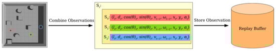
Figure 1.
Preparation schematic visualizing an example of an observation with three agents. Each agent’s individual information is recorded and stored as a part of a single-state observation . Afterward, the state observation is stored in the replay buffer as a single entry.
For an agent to reason about an interaction with other agents in the scene, the information needs to be given relative to its current state. More specifically, the spatial relations need to be given according to the ego agent’s pose in its frame of reference. Not only does this explicitly model the relative interaction, but it also allows for the generalization of interaction information independent of global scene information. To achieve this, the information in the recorded observation tuple needs to be processed before it can be used in neural network training. For each agent, the features of other agents need to be transformed in its frame of reference. With slight abuse of notation, we will borrow the terms of node and edge features from graph neural network (GNN) literature, where the node features are the observation features of the ego agent and edge features are other agent features. As node features N from (2) we use the features that are expressed in ego agents frame:
For each agent in the scene, edge features E are calculated from information in (2) for every other agent:
Here, linear and angular velocities are taken directly from the stored tuple from (2). The relative distance is calculated as the Euclidean distance between x and y positions of each agent. The heading towards the agent is expressed as and and calculated with (3) and (4), respectively, by replacing the heading towards goal with the vector towards the agent location . A similar method is applied when calculating the difference between the heading of the ego agent and the heading of the other agent. This data processing method prepares all the incoming edge data relative to the ego agent in its frame of reference. This process is visualized in Figure 2.
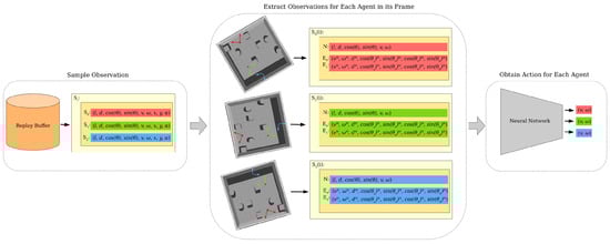
Figure 2.
Example of observation preparation into node and edge information in a scene with three agents. First, a state observation is sampled from the replay buffer. Node and edge information is formed for each agent in its frame of reference to create an individual sample from each agent’s perspective. Each created sample is then used in a neural network to update the learned policy.
4.2. Model Architecture
As base model architecture, we use the TD3-based implementation discussed in our previous work in [6]. However, we make slight changes to the layer layout and activation functions. Moreover, since we are also considering the incoming edge information from other agents, this information needs to be embedded and combined with the node information. To achieve this, we design a local edge information embedder sub-graph. Since the number of agents in the scene that may interact with the ego agent is dynamic, this sub-graph must be capable of including varied size inputs. We achieve this by batching all incoming edge information E into a single batch with n dimensions. This batch is then passed through a sequence of embedding layers consisting of sequential, fully connected and continuously differentiable exponential linear unit (CELU) [38] activation layers. This process returns n-dimensional embedding of all incoming edges. In order to obtain single-dimension embedding information for all edges, we perform maximum value aggregation over all embeddings. This aggregation returns the maximal value of each feature embedding in a single vector representation of all other agents in the scene. The edge information embedder sub-graph structure is visualized in Figure 3.
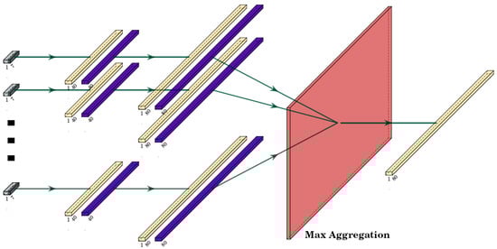
Figure 3.
Edge embedder layer structure for n-dimensional input of other agent information. The edge information is passed through a series of fully connected layers, all sharing the same weights. Fully connected layers are represented in yellow and CELU in purple. Max aggregation (visualized in red) is used to aggregate the encoded information to a single-dimension output.
The input to the neural network consists of ego agent features and a batch of other agent features, as described in Section 4.1 for every robot in the scene. The actor part of the neural network embeds the ego agent features with a fully connected linear layer followed by CELU activation function. The batch of other agent features is embedded using the sub-graph. The ego agent and other agent embeddings are concatenated, followed by a fully connected layer and a CELU activation layer. Finally, another fully connected layer follows with a hyperbolic tangent (Tanh) activation function that constrains the output to [−1, 1] range. The actor–network output is a two-dimensional vector representing the obtained linear and angular velocities for the ego agent. The actor–network structure is depicted in Figure 4, and the layers are described in Table 1.

Figure 4.
Actor–network structure. Inputs of ego agent and other agent information are depicted in gray. Edge embedder described in Figure 5 is stylized in light red. Fully connected layers are represented in yellow and CELU in dark purple, with Tanh activation in light purple. Concatenation, which combines the ego agent features with embedded edge features, is represented with the green circle. Here, the action calculated in the actor network is also used as an input to calculate state–action pair value. It is passed directly into the TFC layer, which is depicted in a light green color.

Table 1.
Network parameters and structure of actor network.
The chosen TD3 implementation uses two critics to mitigate the value overestimation often present in deep deterministic policy gradient (DDPG) neural networks [39]. Therefore, we implement two critics with the same layer structure. The critic networks have a similar architecture to the actor network. We embed the ego agent features and other agent features with their respective embedders. After concatenation, we obtain a single-dimension embedding of all the state information. Then, this information is passed through a single fully connected linear layer. Critic networks also take as an input the action calculated by the actor network for the same state information. This information is passed through a fully connected layer. Then, the output from state and action embeddings is combined using a transformation fully connected (TFC) layer as described in [40], which is followed by the activation function. Finally, a Q-value decoder obtains an estimated state–action pair value. The full critic network structure is depicted in Figure 5, and the parameter values are described in Table 2.
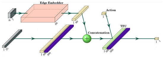
Figure 5.
Critic network structure. Inputs of ego agent and other agent information are depicted in gray. Edge embedder described in Figure 5 is stylized in light red. Fully connected layers are represented in yellow and CELU in dark purple. Concatenation, which combines the ego agent features with embedded edge features, is represented with the green circle.
Table 2.
Network parameters and structure of both critic networks.
5. Training
We use a simulation to train the neural network described in Section 4. This allows the neural network to be trained with unambiguous information, as well as easing the information exchange between the agents. Since it is possible to simultaneously obtain actions for all agents in the scene, we employ a method of policy training in which observations are recorded from all participants in the environment. We collect multiple state samples for each time step in the simulator and calculate the action for all of them based on the current policy. Moreover, the neural network can learn through interactions with its policy.
5.1. Simulation Setup
The gazebo simulator facilitates obtain state observation as well as action execution. The Robot Operating System (ROS) is used as a bridge between the neural network and the simulator. For training, we use a 10 by 10-m walled environment. In the environment, we place multiple large cubes and cylinders, and their location is randomized at the beginning of every episode to increase the scene variance and improve the methods’ generalizability. The actions are executed on simulated turtlebot 3 [41] differential drive robot models that serve as agents for our neural network. Neural network outputs are communicated to robots as ROS Twist-type messages. While the proposed method is generally sensor agnostic, we use laser readings to observe the environment for robot navigation due to the reduced number of returned sensor values and increased field of view compared to depth or RGB camera observations. A simulated Velodyne Puck sensor is placed on each robot, which records laser readings in a 180-degree field of view. This information, along with the robot’s odometry and executed velocities, is used as part of the state information in (2). The goal information for calculating values of d, and is obtained from the simulator. The goal positions, robots’ starting positions and poses are also randomized at the start of each episode as not to overlap with any of the obstacles in the environment. We train the neural network with three robots sharing the environment. The simulation setup is depicted in Figure 6.
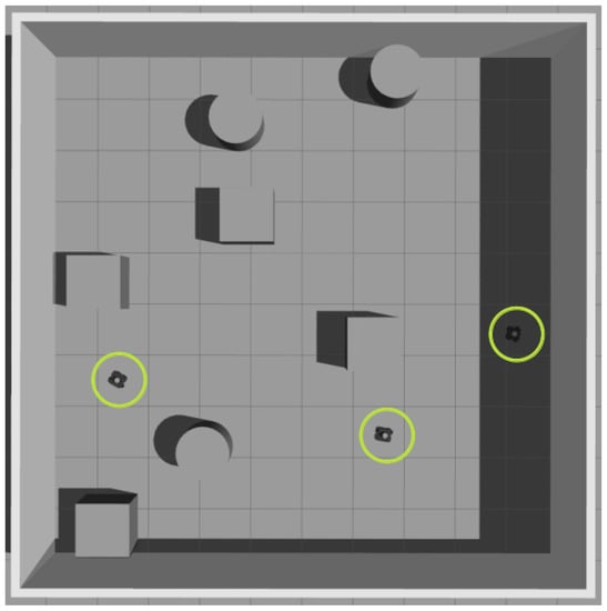
Figure 6.
Gazebo simulator environment used for training neural network policy. Three robots are randomly placed in the environment and shown with green circles around them. Such obstacles as cylinders and boxes are also placed in the environment as obstacles, and their locations are randomized at the start of each episode.
5.2. Training in Simulation
The training setup is executed as follows. A number of robots are initialized in the environment and assigned random goal positions. All robots execute actions given by the current policy of the neural network. While performing actions in the environment, observations in the form of (1) are collected. Once a robot finishes its trajectory, either by colliding with an obstacle or reaching the goal, its terminal state flag is set. In the subsequent time step, its completion flag c is also set, and no further actions will be executed with this robot. However, the robot continues to broadcast its edge information, and it is still used to calculate the actions of other robots. The training episode concludes when all the robots have finished their trajectories or the trajectory time steps exceed a pre-set threshold. After the episode concludes, a batch of observations is sampled from the replay buffer to update the actor and critic network parameters. When updating neural network parameters, each observation is preprocessed according to the description provided in Section 4.1. However, only agents with the unset parameter c are used as ego agents in the data processing, as only agents that are still executing a trajectory receive rewards for their actions. Only these samples are then utilized for loss calculation.
5.3. Training Parameters and Bootstrapping
We employ bootstrapping methods to guide and speed up the training convergence. The basic task of the neural network is to obtain a policy that guides the robot to the goal position. However, since there is only one goal in the environment, there is a low probability that a policy based on randomly initialized weights will be able to reach it. This means that the trajectories with successful goal reaching will be under-represented in the replay buffer. To mitigate this issue, we set a distance threshold of how far a goal position can be randomly placed from its respective robot. We expand this distance every time a robot reaches its goal. Another method employed is adding Gaussian noise to the obtained action from the policy. This allows us to take slightly different actions than the ones calculated and allows for exploration of the policy. We start the training with a set maximum variance for the Gaussian noise and slightly reduce it at every time step. However, Gaussian noise by definition is centered around the already existing policy and, in the majority of cases, will produce very slight deviations from it, especially later in the training process with a small variance. This is conducive to optimizing an already well-behaving policy. But there are cases in which drastically different actions could produce more positive outcomes in the long run. Therefore, for time steps that satisfy the criteria:
where R is a random scalar drawn in the range , we take a completely random action drawn from a uniform distribution. This allows us to randomly take out-of-distribution actions while still generally executing trajectories following the policy.
The reinforcement algorithm uses rewards to evaluate performance. In our training setup, we employ the following reward function:
Here, is the reward for reaching the goal when the distance to the goal from the robot is below a threshold . The collision reward is given when the minimum laser reading is below a threshold . The immediate reward is calculated as:
where is the coefficient for the respective reward element and is a negative reward depending on closeness to obstacles, obtained as follows:
where is a threshold for the distance to obstacles. The full list of training parameters is available in Table 3.
Table 3.
Network parameters and structure of both critic networks.
6. Experiments
We conducted a series of experiments in a simulated environment to validate our approach. We designed six scenarios in which multiple robots must simultaneously navigate to their designated goal positions without colliding. To emphasize the versatility of our approach in handling environments with varying number of actors, each scenario was executed with two, three, and four controlled robots, respectively. The scenario setup is depicted in Figure 7, illustrating the starting positions, headings, and goal positions of the four robots. The same setup was used for experiments involving fewer robots. Each experiment was repeated 20 times. While the learned model policy is deterministic, the simulation is not due to the imprecise timing of message exchanges. As a result, each run yielded in a slightly different trajectory. This feature enabled us to evaluate the generalizability and adaptivity of our proposed method. To refer conveniently to our method, we coined the name you are not alone (YANA). To compare YANA, we performed a direct comparison with an ablated neural network architecture similar to those used in [15,40], where a neural network is trained for mobile robot navigation in unknown environments. We implemented the network architecture in a manner consistent with the referenced papers, with CELU activation layers to align them with our approach. We trained this neural network in the same conditions as YANA, employing the same bootstrapping methods and environment setup. This network model was also trained in a shared environment, simultaneously collecting trajectories from three robots. As this method was trained in a shared environment but lacked an information exchange between scene actors, we denote it as you are (not) alone (YA(n)A). Given that learned behaviors in shared environments might also exhibit interaction patterns, we further validate the results against the standard TD3 implementation. In this case, network training was conducted with static obstacles and a single robot in the scene, while retaining the same training setup otherwise. The best-performing performing models after 100 epochs of training were compared for each experiment scenario. All robots in the experimental setup were controlled by their respective policies. As evaluation metrics, we computed the average combined distance traveled, the average combined number of steps and the average collisions, along with their respective standard deviations for each experiment setting. The unit of distance is expressed in meters.
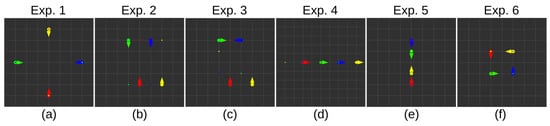
Figure 7.
Simulated experiment setup. Figures (a–f) visualize each robot’s starting position and heading for each respective experiment. Large circles represent the robot’s starting position and the arrows represent their heading. Smaller circles represent goal points for robots of the same color. The grid is represented with 1 by 1 meter-sized squares.
6.1. Experiments with 2 Robots
First, we perform the experiments in a setting with two robots. The starting positions and poses of the robots are visualized in Figure 7, although only two robots are initialized. We collect trajectories and metrics for all three compared methods, presented in Table 4. A representative sample of trajectories is visualized in Figure 8. Observing the experiments, it becomes evident that the proposed YANA method effectively avoids and anticipates the motion of another agent in the scene. While other approaches (YA(n)A and base TD3) succeed in most cases, collisions occur in specific scenarios. For YA(n)A in Experiments 1 and 5, the robots occasionally arrive at a single location simultaneously, lacking a learned exchange strategy that results in collisions. In the TD3 case, an issue arises in Experiment 2 due to an approaching frontal obstacle. The training environment featured solely static obstacles, rendering frontal dynamic obstacle avoidance challenging, as the obstacle advances earlier than anticipated. In scenarios in which arriving at the goal was always successful, distance data indicate that YA(n)A and TD3 select more optimal routes with less consideration for other agents in the scene. Nevertheless, YANA’s distance measurement remains comparable to other approaches. However, comparing the average number of steps taken, YANA exhibits a longer time to reach the goal in certain scenarios. For instance, in Experiment 4, for the robot displayed in red, the YANA approach waits for the green robot to navigate to a safe distance before initiating its own movement. In contrast, YA(n)A and TD3 start navigating towards the goal immediately. From the results, we can see that while YANA outperforms other approaches in terms of safety, YA(n)A and basic TD3 could still be used for robot navigation in this setting, provided that collision strategies are improved.
Table 4.
Experiments with 2 robots.
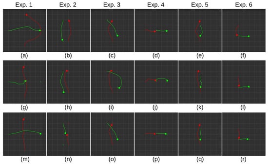
Figure 8.
Experimental results with 2 robots in 6 scenarios. (a–f) Representative recorded trajectories with YANA policy. (g–l) Representative recorded trajectories with YA(n)A policy. (m–r) Representative recorded trajectories with TD3 policy. Robots are represented with a large circle. Their trajectories and goal positions are represented with a line and a smaller circle in their respective colors. Robots not at their goal position represent the point of collision.
6.2. Experiments with 3 Robots
Next, we conducted experiments in the same setting with three robots; the results are presented in Table 5. Representative trajectories from the experiment are visualized in Figure 9. In this scenario, issues with the YA(n)A and TD3 approaches in collision avoidance begin to emerge. Although the YA(n)A method employs a training method with multiple robots in the scene, most instances involve robots moving in separate directions or observing each other from a distance. However, in these experiments, they are forced to intersect paths and avoid collisions in a reasonable manner. The lack of robot exchange strategy becomes evident, as the only experiment in which no collisions were observed is Experiment 2. With the introduction of an additional agent in the scene, the TD3 method also experiences a significantly higher collision rate. In contrast, the YANA method still navigates safely, with a single collision observed in Experiment 5. Comparing distance measurements across approaches in experiments without reported collisions, it is apparent that YANA takes less optimal but more cautious trajectories. It demonstrates a willingness to wait for other robots to pass, as indicated by the average number of steps taken.
Table 5.
Experiments with 3 robots.
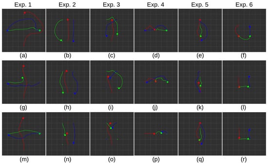
Figure 9.
Experimental results with 3 robots in 6 scenarios. (a–f) Representative recorded trajectories with YANA policy. (g–l) Representative recorded trajectories with YA(n)A policy. (m–r) Representative recorded trajectories with TD3 policy. Robots are represented with a large circle. Their trajectories and goal positions are represented with a line and a smaller circle in their respective colors. Robots not at their goal position represent the point of collision.
6.3. Experiments with 4 Robots
To demonstrate the advantages of the proposed approach when dealing with a greater number of scene agents, we conducted experiments with four robots; the results are presented in Table 6. Representative trajectories are visualized in Figure 10. Here, we can observe a larger increase in collisions for YA(n)A and TD3 methods. However, there is one additional collision also observed in the case of the YANA method in Experiment 3. Nonetheless, this figure remains notably lower compared to the collision occurrences in the other methods, particularly in a relatively intricate scenario involving robot exchanges. As the number of agents increases, making determinations concerning distance and step information becomes more challenging, since the other approaches struggle to achieve collision-free navigation in most scenarios. Despite this, we can still draw similar conclusions to those derived from the Experiments with two and three robots.
Table 6.
Experiments with 4 robots.
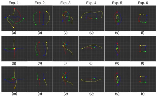
Figure 10.
Experimental results with 4 robots in 6 scenarios. (a–f) Representative recorded trajectories with YANA policy. (g–l) Representative recorded trajectories with YA(n)A policy. (m–r) Representative recorded trajectories with TD3 policy. Robots are represented with a large circle. Their trajectories and goal positions are represented with a line and a smaller circle in their respective colors. Robots not at their goal position, represent the point of collision.
7. Summary and Conclusions
In this paper, we presented a novel approach used to train a mobile robot policy in shared environments. We presented an approach for training a generalizable policy, collecting data, and its transformation into translation and rotation invariant features. By design, our proposed method can be adapted to handle a varying number of scene agents and to devise interaction policies from an ego vehicle perspective. This implies that each agent in the scene can make intelligent motion decisions independently, eliminating the need for an overarching planner for interaction modeling. Through experiments, we demonstrate the benefits of the proposed network architecture and training methodology. We also emphasize that simply training a policy in shared environments is not enough to obtain a well-performing motion policy.
The edge embedder method highlights the advantages of a direct exchange between agents in the scene. However, determining representative features of other agents remains an open question and is highly dependent on the capabilities of the robot. In this paper, we select features that could theoretically be extracted from sequential LiDAR observations in the floor-cleaning domain. These features can only represent the observable state of other agents, not their internal structure or tasks. Additional features might benefit from obtaining more optimal motion policies and exchange strategies. For instance, knowledge of other agents’ goal positions might help the ego agent to reason about its motion, considering whether to wait for another agent to pass or take an alternate route. However, such information exchange would require a direct line of communication between robots in the scene, the implementation of which is outside the scope of this paper. Another potential issue is the noise in observable data. While the proposed method assumes sample independence and therefore sequential steps do not influence each other, real-world settings could involve such features as speed and velocity, which are detectable from sequential steps. To address this, data filtering methods, such as introducing Kalman filtering or training with temporal layers like long short-term memory (LSTM) or gated recurrent unit (GRU), could be introduced.
In future, we aim to implement and test this approach in real-life settings with differential drive robots. Additionally, in our training settings, we aim to use pre-trained policies based on human motion to better learn interaction policies, creating a closer resemblance to interactions with human-operated robotic devices. We plan to utilize a method outlined in our previous work [6], where a reward function is based on observed human motion. Then, a single robot could be used to implement optimal floor cleaning robot policy using edge information. This policy will be rolled out in a simulation environment in which other agents utilize pre-trained, human-like policies. This strategy could narrow the simulation-to-reality gap for cleaning robot navigation and facilitate improved human–robot interaction in shared spaces. These are the planned future steps of our research.
Author Contributions
Conceptualization, R.C. and M.B.; methodology, R.C.; software, R.C. and V.T.; validation, R.C., V.T. and A.K.; resources, V.T., M.B. and A.K.; writing—original draft preparation, R.C., V.T. and A.K.; writing—review and editing, M.B.; visualization, R.C.; project administration, M.B.; funding acquisition, M.B. All authors have read and agreed to the published version of the manuscript.
Funding
This research was funded by the European Regional Development Fund within the project “Clean 4.0—accelerating the adoption of autonomous technologies across the European cleaning ecosystem”, grant number 1.1.1.1/20/A/186.
Institutional Review Board Statement
Not applicable.
Informed Consent Statement
Not applicable.
Data Availability Statement
Data sharing not applicable. No new data were created or analyzed in this study. Data sharing is not applicable to this article.
Conflicts of Interest
The authors declare no conflict of interest.
Abbreviations
The following abbreviations are used in this manuscript:
| DRL | Deep Reinforcement Learning. |
| DL | Deep Learning. |
| DQN | Deep Q-Network. |
| SAC | Soft Actor–Critic. |
| DDPG | Deep Deterministic Policy Gradient. |
| TD3 | Twin Delayed Deep Deterministic Policy Gradient. |
| GNN | Graph Neural Network. |
| MDP | Markov Decision Process. |
| CELU | Continuously Differentiable Exponential Linear Unit. |
| Tanh | Hyperbolic Tangent. |
| TFC | Transformation Fully Connected. |
| ROS | Robot Operating System. |
| YANA | You Are Not Alone. |
| YA(n)A | You Are (not) Alone. |
| LSTM | Long Short-Term Memory. |
| GRU | Gated Recurrent Unit. |
References
- DeSouza, G.N.; Kak, A.C. Vision for mobile robot navigation: A survey. IEEE Trans. Pattern Anal. Mach. Intell. 2002, 24, 237–267. [Google Scholar] [CrossRef]
- Pandey, A.; Pandey, S.; Parhi, D. Mobile robot navigation and obstacle avoidance techniques: A review. Int. Robot. Autom. J. 2017, 2, 96–105. [Google Scholar] [CrossRef]
- Xiao, X.; Liu, B.; Warnell, G.; Stone, P. Motion planning and control for mobile robot navigation using machine learning: A survey. Auton. Robot. 2022, 46, 569–597. [Google Scholar] [CrossRef]
- Zhu, K.; Zhang, T. Deep reinforcement learning based mobile robot navigation: A review. Tsinghua Sci. Technol. 2021, 26, 674–691. [Google Scholar] [CrossRef]
- Shi, Y.; Li, L.; Yang, J.; Wang, Y.; Hao, S. Center-based transfer feature learning with classifier adaptation for surface defect recognition. Mech. Syst. Signal Process. 2023, 188, 110001. [Google Scholar] [CrossRef]
- Cimurs, R.; Merchán-Cruz, E.A. Leveraging Expert Demonstration Features for Deep Reinforcement Learning in Floor Cleaning Robot Navigation. Sensors 2022, 22, 7750. [Google Scholar] [CrossRef]
- Jiang, H.; Wang, H.; Yau, W.Y.; Wan, K.W. A brief survey: Deep reinforcement learning in mobile robot navigation. In Proceedings of the 2020 15th IEEE Conference on Industrial Electronics and Applications (ICIEA), Kristiansand, Norway, 9–13 November 2020; pp. 592–597. [Google Scholar]
- Ruan, X.; Ren, D.; Zhu, X.; Huang, J. Mobile robot navigation based on deep reinforcement learning. In Proceedings of the 2019 Chinese Control and Decision Conference (CCDC), Nanchang, China, 3–5 June 2019; pp. 6174–6178. [Google Scholar]
- Xue, X.; Li, Z.; Zhang, D.; Yan, Y. A deep reinforcement learning method for mobile robot collision avoidance based on double dqn. In Proceedings of the 2019 IEEE 28th International Symposium on Industrial Electronics (ISIE), Vancouver, BC, Canada, 12–14 June 2019; pp. 2131–2136. [Google Scholar]
- Sasaki, H.; Horiuchi, T.; Kato, S. A study on vision-based mobile robot learning by deep Q-network. In Proceedings of the 2017 56th Annual Conference of the Society of Instrument and Control Engineers of Japan (SICE), Kanazawa, Japan, 19–22 September 2017; pp. 799–804. [Google Scholar]
- Xie, L.; Wang, S.; Markham, A.; Trigoni, N. Towards Monocular Vision based Obstacle Avoidance through Deep Reinforcement Learning. arXiv 2017, arXiv:1706.09829. [Google Scholar]
- Xiang, J.; Li, Q.; Dong, X.; Ren, Z. Continuous control with deep reinforcement learning for mobile robot navigation. In Proceedings of the 2019 Chinese Automation Congress (CAC), Hangzhou, China, 22–24 November 2019; pp. 1501–1506. [Google Scholar]
- de Jesus, J.C.; Kich, V.A.; Kolling, A.H.; Grando, R.B.; Cuadros, M.A.d.S.L.; Gamarra, D.F.T. Soft actor-critic for navigation of mobile robots. J. Intell. Robot. Syst. 2021, 102, 1–11. [Google Scholar] [CrossRef]
- Tang, Y.; Zhao, C.; Wang, J.; Zhang, C.; Sun, Q.; Zheng, W.X.; Du, W.; Qian, F.; Kurths, J. Perception and navigation in autonomous systems in the era of learning: A survey. IEEE Trans. Neural Netw. Learn. Syst. 2022, 1–12. [Google Scholar] [CrossRef]
- Tai, L.; Paolo, G.; Liu, M. Virtual-to-real deep reinforcement learning: Continuous control of mobile robots for mapless navigation. In Proceedings of the 2017 IEEE/RSJ International Conference on Intelligent Robots and Systems (IROS), Vancouver, BC, Canada, 24–28 September 2017; pp. 31–36. [Google Scholar]
- Dankwa, S.; Zheng, W. Twin-delayed ddpg: A deep reinforcement learning technique to model a continuous movement of an intelligent robot agent. In Proceedings of the 3rd International Conference on Vision, Image and Signal Processing, Vancouver, BC, Canada, 26–28 August 2019; pp. 1–5. [Google Scholar]
- Kim, M.; Han, D.K.; Park, J.H.; Kim, J.S. Motion planning of robot manipulators for a smoother path using a twin delayed deep deterministic policy gradient with hindsight experience replay. Appl. Sci. 2020, 10, 575. [Google Scholar] [CrossRef]
- Gao, J.; Ye, W.; Guo, J.; Li, Z. Deep reinforcement learning for indoor mobile robot path planning. Sensors 2020, 20, 5493. [Google Scholar] [CrossRef] [PubMed]
- Xianjia, Y.; Queralta, J.P.; Heikkonen, J.; Westerlund, T. Federated learning in robotic and autonomous systems. Procedia Comput. Sci. 2021, 191, 135–142. [Google Scholar] [CrossRef]
- Dias, P.G.F.; Silva, M.C.; Rocha Filho, G.P.; Vargas, P.A.; Cota, L.P.; Pessin, G. Swarm robotics: A perspective on the latest reviewed concepts and applications. Sensors 2021, 21, 2062. [Google Scholar] [CrossRef] [PubMed]
- Liu, B.; Wang, L.; Liu, M. Lifelong federated reinforcement learning: A learning architecture for navigation in cloud robotic systems. IEEE Robot. Autom. Lett. 2019, 4, 4555–4562. [Google Scholar] [CrossRef]
- Rajaratnam, D.; Schaub, T.; Wanko, P.; Chen, K.; Liu, S.; Son, T.C. Solving an Industrial-Scale Warehouse Delivery Problem with Answer Set Programming Modulo Difference Constraints. Algorithms 2023, 16, 216. [Google Scholar] [CrossRef]
- Connor, J.; Champion, B.; Joordens, M.A. Current algorithms, communication methods and designs for underwater swarm robotics: A review. IEEE Sens. J. 2020, 21, 153–169. [Google Scholar] [CrossRef]
- Dorigo, M.; Theraulaz, G.; Trianni, V. Swarm robotics: Past, present, and future [point of view]. Proc. IEEE 2021, 109, 1152–1165. [Google Scholar] [CrossRef]
- Calderón-Arce, C.; Brenes-Torres, J.C.; Solis-Ortega, R. Swarm robotics: Simulators, platforms and applications review. Computation 2022, 10, 80. [Google Scholar] [CrossRef]
- Zhang, M.; Yang, B. Swarm robots cooperative and persistent distribution modeling and optimization based on the smart community logistics service framework. Algorithms 2022, 15, 39. [Google Scholar] [CrossRef]
- Boldrer, M.; Antonucci, A.; Bevilacqua, P.; Palopoli, L.; Fontanelli, D. Multi-agent navigation in human-shared environments: A safe and socially-aware approach. Robot. Auton. Syst. 2022, 149, 103979. [Google Scholar] [CrossRef]
- Klančar, G.; Seder, M. Coordinated Multi-Robotic Vehicles Navigation and Control in Shop Floor Automation. Sensors 2022, 22, 1455. [Google Scholar] [CrossRef] [PubMed]
- Şenbaşlar, B.; Sukhatme, G.S. Asynchronous Real-time Decentralized Multi-Robot Trajectory Planning. In Proceedings of the 2022 IEEE/RSJ International Conference on Intelligent Robots and Systems (IROS), Kyoto, Japan, 23–27 October 2022; pp. 9972–9979. [Google Scholar]
- Scarselli, F.; Gori, M.; Tsoi, A.C.; Hagenbuchner, M.; Monfardini, G. The graph neural network model. IEEE Trans. Neural Netw. 2008, 20, 61–80. [Google Scholar] [CrossRef]
- Veličković, P. Everything is connected: Graph neural networks. Curr. Opin. Struct. Biol. 2023, 79, 102538. [Google Scholar] [CrossRef] [PubMed]
- Li, Q.; Gama, F.; Ribeiro, A.; Prorok, A. Graph neural networks for decentralized multi-robot path planning. In Proceedings of the 2020 IEEE/RSJ International Conference on Intelligent Robots and Systems (IROS), Las Vegas, NV, USA, 24 October 2020–24 January 2021; pp. 11785–11792. [Google Scholar]
- Li, Q.; Lin, W.; Liu, Z.; Prorok, A. Message-aware graph attention networks for large-scale multi-robot path planning. IEEE Robot. Autom. Lett. 2021, 6, 5533–5540. [Google Scholar] [CrossRef]
- Lin, S.; Liu, A.; Wang, J.; Kong, X. A review of path-planning approaches for multiple mobile robots. Machines 2022, 10, 773. [Google Scholar] [CrossRef]
- Zaheer, M.; Kottur, S.; Ravanbakhsh, S.; Poczos, B.; Salakhutdinov, R.R.; Smola, A.J. Deep sets. Adv. Neural Inf. Process. Syst. 2017, 30, 1–11. [Google Scholar]
- Karch, T.; Colas, C.; Teodorescu, L.; Moulin-Frier, C.; Oudeyer, P.Y. Deep sets for generalization in rl. arXiv 2020, arXiv:2003.09443. [Google Scholar]
- Liu, Z.; Yang, D.; Wang, Y.; Lu, M.; Li, R. EGNN: Graph structure learning based on evolutionary computation helps more in graph neural networks. Appl. Soft Comput. 2023, 135, 110040. [Google Scholar] [CrossRef]
- Barron, J.T. Continuously differentiable exponential linear units. arXiv 2017, arXiv:1704.07483. [Google Scholar]
- Fujimoto, S.; Hoof, H.; Meger, D. Addressing function approximation error in actor-critic methods. In Proceedings of the International Conference on Machine Learning, Stockholm, Sweden, 10–15 July 2018; pp. 1587–1596. [Google Scholar]
- Cimurs, R.; Suh, I.H.; Lee, J.H. Goal-driven autonomous exploration through deep reinforcement learning. IEEE Robot. Autom. Lett. 2021, 7, 730–737. [Google Scholar] [CrossRef]
- Amsters, R.; Slaets, P. Turtlebot 3 as a robotics education platform. In Robotics in Education: Current Research and Innovations 10; Springer: Berlin/Heidelberg, Germany, 2020; pp. 170–181. [Google Scholar]
Disclaimer/Publisher’s Note: The statements, opinions and data contained in all publications are solely those of the individual author(s) and contributor(s) and not of MDPI and/or the editor(s). MDPI and/or the editor(s) disclaim responsibility for any injury to people or property resulting from any ideas, methods, instructions or products referred to in the content. |
© 2023 by the authors. Licensee MDPI, Basel, Switzerland. This article is an open access article distributed under the terms and conditions of the Creative Commons Attribution (CC BY) license (https://creativecommons.org/licenses/by/4.0/).