Two Medoid-Based Algorithms for Clustering Sets

Abstract

This paper proposes two algorithms for clustering data, which are variable-sized sets of elementary items. An example of such data occurs in the analysis of a medical diagnosis, where the goal is to detect human subjects who share common diseases to possibly predict future illnesses from previous medical history. The first proposed algorithm is based on K-medoids and the second algorithm extends the random swap algorithm, which has proven to be capable of efficient and careful clustering; both algorithms depend on a distance function among data objects (sets), which can use application-sensitive weights or priorities. The proposed distance function makes it possible to exploit several seeding methods that can improve clustering accuracy. A key factor in the two algorithms is their parallel implementation in Java, based on functional programming using streams and lambda expressions. The use of parallelism smooths out the $O(N^2)$ computational cost behind K-medoids and clustering indexes such as the Silhouette index and allows for the handling of non-trivial datasets. This paper applies the algorithms to several benchmark case studies of sets and demonstrates how accurate and time-efficient clustering solutions can be achieved.

1. Introduction

Unsupervised clustering aims to group data into clusters in such a way that data within the same cluster are similar to each other, and data in different clusters are dissimilar.

K-means [1,2] is a widely used clustering algorithm due to its simplicity and efficiency. Another reason to prefer K-means instead of a more sophisticated algorithm is the fact that its properties and limitations have been thoroughly investigated [3,4]. Two main limitations of K-means are that (1) it operates on numerical data using Euclidean distance and (2) it requires calculation of the mean of the objects (centroid) in the set.

Dealing with data that have mixed numerical and categorical attributes or only categorical attributes is difficult [5]. Such data can be handled either by preliminarily converting, most often in an unnatural way that can imply sparsity and multi-dimensional problem, categorical attributes to numerical ones, or by introducing a non-Euclidean distance function.

Adapting K-means to deal with data objects which are sets of elementary items [6] poses similar problems to coping with categorical attributes. In addition, the need exists to handle sets of different sizes.

A histogram-based approach has been used for clustering categorical data [5,7] and recently for clustering sets [8]. The idea is to use a histogram of the categorical values to represent the cluster. This eliminates the need to define the mean value. In the case of categorical data, the distance to the cluster can be defined based on the frequency of the category labels of the object in the cluster. In the case of sets, the distance between objects and the clusters can be derived from classical set-matching measures such as Jaccard and Otsuka–Ochiai cosine distance [8].

As a practical example of an application of clustering sets, the records of medical patient diagnoses can be considered, where the goal is to find groups of similar patients to support the estimation of the risk for a patient to develop some future illness due to his/her previous medical history and from correlations to other patients with similar diseases.

In this paper, we propose a new approach for clustering sets which is based on K-medoids. Medoid is the object in the cluster having a minimum total distance from all other objects in the cluster. Then, all we need is a distance measure between the objects. Since both the data and the cluster representative (medoid) are sets, we can apply the classical set-distance measures slightly modified, as in [8], by considering application-sensitive information.

We apply the medoid approach within two clustering algorithms: K-medoids [9,10] and random swap [11,12]. The proposed approach retains the generality and effectiveness of the corresponding K-sets and K-swaps algorithms described in [8] at the cost of a somewhat slower running time.

The original contributions provided by this paper are the following:

• Introducing two new algorithms for clustering sets: K-medoids and random swap using medoid and the two classical set-matching distances of Jaccard and Otsuka–Ochiai cosine coefficients [13], adapted by considering the frequency of use of the items in the whole dataset.
• Exploring the effect of random initialization versus K-means++ initialization [14,15,16,17,18].
• Implementing parallel variants using Java parallel streams and lambda expressions [12,19,20], which provide better time efficiency on a multi-core machine.

The effectiveness of the new approach is demonstrated by applying it to the 15 synthetic datasets used in [8]. The algorithms both achieve good clustering quality, which is very similar to that of the previous K-swaps algorithm. However, the proposed medoid-based approach is simpler to implement, and it avoids the threshold parameter for truncating the histogram size. While this might not be the big issue with most data, there are always some potential pathological cases that the proposed approach is likely to avoid.

This paper is organized as follows: Section 2 summarizes the previous work on adopting K-means to the sets of data; Section 3 describes the proposed algorithms for clustering sets based on medoids, together with some Java implementation issues; Section 4 describes the experimental setup; Section 5 reports the achieved clustering results; Section 6 concludes this paper by highlighting some directions for further work.

2. Related Work

In this section, the work of [8] is summarized as the fundamental background upon which the new approach proposed in this paper is based. For further related work the reader is referred to [8].

A dataset consists of variable-sized sets of elementary items taken from a vocabulary of size $L$ (which is said to be the problem resolution). Practical data can be the records of patient diagnoses expressed by ICD-10 [8,21] disease codes, preliminarily grouped by similar diseases, for medical applications.

To each cluster a representative data object (centroid) is associated in the form of a histogram which records the frequency of each item occurring in the cluster. A histogram contains at most m = 20 distinct items. For clusters with more items, the m most frequent items are selected. To apply K-means clustering, a distance measure between a data object (a set) $X$ of size $l$ and a representative histogram $h$ must be defined. In [8], adapted versions of the Jaccard or the Otsuka–Ochiai cosine distance were introduced. Adaptation is needed because in the case of large values of $L$, an intersection between two sets may contain only a few common elements, and the distance measure becomes meaningless. A weight is, therefore, defined as the frequency of the item in the local histogram $h$.

The two distance notions (Jaccard and cosine) are defined accordingly:

$$d_J\left(X,h\right)=1-\frac{{{\displaystyle \sum }}_{x_i\in X\&x_i\in h}{f}_h\left(x_i\right)}{{{\displaystyle \sum }}_{y_i\in h}{f}_h\left(y_i\right)+{{\displaystyle \sum }}_{x_i\in X,x_i\notin h}1}$$

(1)

$$d_C\left(X,h\right)=1-\frac{{{\displaystyle \sum }}_{x_i\in X\&x_i\in h}{f}_h\left(x_i\right)}{\sqrt{{{\displaystyle \sum }}_{y_i\in h}{\left(f_h\left(y_i\right)\right)}^2}\ast \sqrt{l}}$$

(2)

2.1. Example

The following example, taken from [8], refers to a cluster with five data objects that are sets of elementary items denoted by a single capital letter:

$$\begin{array}{c}{X}_1=\left\{A,E,B,C,F\right\}\\ X_2=\left\{D,G,A,B\right\}\\ X_3=\left\{A,H,C,B\right\}\\ X_4=\left\{I,A,C,J,B\right\}\\ X_5=\left\{B,D,C,A\right\}\end{array}$$

The approach in [8] first associates the representative (centroid) to the cluster in the form of a histogram with local frequencies of use of the data items, thus:

$h$:

A	B	C	D	E	F	G	H	I	J
5	5	4	2	1	1	1	1	1	1

Since the number of distinct data items in the cluster (10) is less than 20, all items of the data objects are included in $h$. Then, the distances of the data objects to the representative can be calculated by (1) or (2). For example:

$$\begin{array}{c}{d}_J\left(X_1,h\right)=1-\frac{f_h\left(A\right)+f_h\left(E\right)+f_h\left(B\right)+f_h\left(C\right)+f_h\left(F\right)}{{{\displaystyle \sum }}_{y_i\in h}{f}_h\left(y_i\right)}=1-\frac{5+1+5+4+1}{22}=1-\frac{16}{22}=0.27\\ d_C\left(X_1,h\right)=1-\frac{16}{\sqrt{5^2+5^2+4^2+2^2+6}\ast \sqrt{5}}=1-\frac{16}{\sqrt{76}\ast \sqrt{5}}=1-0.819=0.18\end{array}$$

These distance measures are used to detect the nearest representative of a data object and to evaluate the contribution of a cluster to the sum of distances to histogram ($SDH$) function cost: $d_J\left(X_1,h\right)+d_J\left(X_2,h\right)+d_J\left(X_3,h\right)+d_J\left(X_4,h\right)+d_J\left(X_5,h\right)$.

The distance function is the basis of an adaptation of K-means [1,2] and random swap [11,12] to sets.

2.2. K-Sets and K-Swaps

K-sets is the direct adaption of k-means to sets. It initializes the $K$ centroids (representatives) through a uniform random selection in the dataset. The initial representatives have unitary frequency for each component item.

Then, the two basic steps, object assignment and centroids update, are carried out as follows: In the assignment step, each data object (set) is assigned to the cluster according to the nearest centroid rule. In the update step, the representative of each cluster is redefined by calculating the new histogram (of m length) with the number of occurrences of each item in the data objects of the cluster. This operation replaces the classical centroid update of K-means because we cannot compute the mean of the data objects which are variable-sized sets of elementary items. The quality of the clustering is evaluated by the sum of the distances to the histogram ($SDH$):

$$SDH={\displaystyle \sum }_{j=1}^K{\displaystyle \sum }_{X\in C_j}d\left(X,h_j\right)$$

(3)

The two basic steps (assignment and update) are iterated until $SDH$ stabilizes, that is, the difference between the current and previous value of $SDH$ is smaller than a threshold $TH={10}^{-8}$.

Similar modifications were also introduced in the random swap algorithm [11] that result in the so-called K-swaps algorithm [8]. It integrates K-sets in the logic of pursuing a global search strategy via centroids swaps. The initialization step is the same as in K-sets, which is immediately followed by a first partitioning. At each swap iteration, a centroid is randomly chosen among the K representatives, and replaced by a randomly chosen data object in the dataset. After the swap, two K-sets iterations are executed and the corresponding $SDH$ value is evaluated. If the swap improves (reduces) $SDH$, the new centroid configuration is accepted and becomes the current solution for the next swap iteration.

Good clustering results are documented in [8], by applying K-sets and K-swaps to 15 benchmark datasets, referred to as $Sets$ data in [22]. K-swaps resulted in low SDH values and high clustering accuracy, measured in terms of the adjusted rand index (ARI) [23,24] values in the case of all benchmark datasets, and K-sets in the case of most datasets.

3. Medoid-Based Approaches

In the approach proposed in this paper, we use medoid [9,10] as the cluster representative instead of a histogram. Medoid is defined as the data object in the cluster with a minimal sum of the distances to the other data objects in the same cluster. The medoid-based approach has two advantages. First, medoid is a more natural cluster representative than a histogram and does not require any parameters such as the threshold for the histogram size. Second, we can use the same distance measures for sets as in [8] but with an adaption of the measures which considers the global frequency of using elementary items in the application dataset.

Specifically, we present two novel medoid-based algorithms. The first algorithm is the classical K-medoids adopted to the sets. The second algorithm is the random swap variant, in which medoid is used instead of the mean of the objects as the clustering representatives.

3.1. New Distance Functions

A dataset is defined as a set $X$ of $N$ objects, where each object $X_j$ is a set of $l$ items taken from a vocabulary of $L$ distinct items:

$$X_j={\left\{x_{ji}\right\}}_{i=1}^l$$

From the dataset, a global histogram $H$ is built from all the L items and their corresponding frequencies in the dataset, denoted by $f_H\left(x_i\right)$. The global histogram was adopted because the frequency of occurrences of an item (for example the disease code in a medical application) naturally can be interpreted as the relative importance of the item with reference to all the other items. Similar to [8], the global frequency of an item, instead of its local frequency in a cluster, is here used as an application-dependent weight (priority) which replaces 1 when counting, by exact match, the size of the intersection of two sets.

We use two weighted distance functions, Jaccard and Otsuka–Ochiai cosine distance. They are defined as follows:

$$d_J\left(X_1,X_2\right)=1-\frac{{{\displaystyle \sum }}_{x_j}\delta \left(x_j\right)}{{{\displaystyle \sum }}_{x_j}\delta \left(x_j\right)+{{\displaystyle \sum }}_{x_i}\overline{\delta }\left(x_i\right)}$$

(4)

$$d_C\left(X_1,X_2\right)=1-\frac{{{\displaystyle \sum }}_{x_j}\delta \left(x_j\right)}{\sqrt{ {{\displaystyle \sum }}_{x_j}\delta \left(x_j\right)+{{\displaystyle \sum }}_{x_i}{\delta }_1\left(x_i\right)}\times \sqrt{{{\displaystyle \sum }}_{x_j}\delta \left(x_j\right)+{{\displaystyle \sum }}_{x_i}{\delta }_2\left(x_i\right)}}$$

(5)

Here, $\delta \left(x_j\right)=f_H\left(x_j\right)$ if $x_j\in X_1{{\displaystyle \cap }}^{\hspace{1em}}{X}_2$, 0 otherwise; $\overline{\delta }\left(x_i\right)=1$ if $x_i\notin X_1{{\displaystyle \cap }}^{\hspace{1em}}{X}_2$, 0 otherwise; ${\delta }_1\left(x_i\right)=1$ if $x_i\in X_1\backslash X_2$, 0 otherwise; ${\delta }_2\left(x_i\right)=1$ if $x_i\in X_2\backslash X_1$, 0 otherwise. So, the maximal distance between two sets is 1 and the minimal one is 0. If the weights of items evaluate to 1, the two distance measures reduce to the standard Jaccard and cosine distances.

The use of modified $d_J$ or $d_C$ distance measure, enables K-medoids [9,10] (see Algorithm 1) and random swap [11,12] (see Algorithm 2) to easily adapt to sets, and also to possibly exploit careful seeding methods.

Algorithm 1: Pseudo-code of K-Medoids for sets

Input: The dataset $X$ and the number $K$ of required clusters

Output: The partitions and medoids of the emerged clustering solution, together with some accuracy measures including the $SDM$ cost

1. Initialization. Initialize the $K$ medoids by a certain seeding method

2. Partitioning: Assign each data object $X_i\in X$ to the cluster $C_j$, if $m_j=nm\left(X_i\right)$

3. Update. Define the new medoid of each cluster as that data object ${m^{\prime }}_j$ which has minimal sum of the distances from all the remaining points of the cluster: ${m^{\prime }}_j{|}_{j=1}^K=Y\in C_j : Y=argmi{n}_{X_p\in C_j} {\displaystyle \sum }_{X_i\in C_j,X_p\ne X_i}d\left(X_p,X_i\right)$

4. Check termination. If medoids are not stable, restart from Step 2; otherwise stop

Algorithm 2: Pseudo-code of Random Swap for sets

Input: The dataset $X$ and the number $K$ of required clusters

Output: The partitions and medoids of the emerged clustering solution, together with some accuracy measures including the $SDM$ cost

1. Initialization. Initialize the $K$ medoids by a certain seeding method

2. Initial Partitioning. Assign data objects to clusters according to the nearest initial medoids; $previous\_cost=SDM$

Repeat $T$ times:

3. Swap. A medoid is uniform randomly chosen in the vector of medoids, and it gets replaced by a data object uniform randomly chosen in the dataset: $$m_s \leftarrow X_i , s=rand\left(1,K\right), i=rand\left(1,N\right)$$     4. Medoids refinement. A few iterations of K-medoids (Algorithm 1) are executed to refine medoids; $curren{t}_{cost}=SDM$     5. Test. If($current\_cost<previous\_cost)$ then the new solution is accepted and becomes current for the next iteration, with $previous\_cost=current\_cost$; otherwise, previous medoids and corresponding partitioning are restored. End Repeat

As in [8], the total sum of distances to medoids ($SDM$) objective function is assumed to be minimized by clusters. Let $\left\{C_1,C_2,\dots ,C_K\right\}$ denote the $K$ clusters and $\left\{m_1,m_2,\dots ,m_K\right\}$ be the corresponding medoid data objects. SDM is defined as:

$$SDM={\displaystyle \sum }_{i=1}^N{\displaystyle \sum }_{X_i\in C_j}d\left(X_i,m_j\right)$$

where $m_j=nm\left(X_i\right)$ is the nearest medoid to the data object $X_i$, that is:

$$m_j=nm\left(X_i\right) \mathrm{with} j=argmi{n}_{1\le h\le K} d\left(X_i,m_h\right).$$

3.2. K-Medoids Algorithm for Sets

Algorithm 1 describes the steps of the algorithm in pseudo-code which differs from the Lloyd’s classical K-means only in the Update step, where instead of computing the mean of the points associated with a cluster, the medoid of the cluster is identified.

The two steps, Steps 2 and 3, are repeated until the medoids stop moving. The computational cost of the algorithm is $O\left(N^{2}KT\right)$ where $T$ is the number of iterations. The cost is dominated by the $O\left(N^2\right)$ cost for all pairwise distances calculation. The matrix of all pairwise distances can be built for tiny datasets in the initialization step. More in general, though, distances between data objects are computed on demand. Therefore, implementation of a parallel algorithm can be required to reduce the computational needs (see later in this paper).

Example

The process of computing medoids can be demonstrated using the cluster example introduced in the Section 2.1. First, the global histogram $H$ of the frequencies of elementary items in the dataset is defined:

$H$:

A	B	C	D	E	F	G	H	I	J	…
35	20	22	20	24	12	10	8	22	7	…

The objects $X_1$ and $X_2$ of the cluster have two items in common ($\mathrm{A},\mathrm{B}$) and five other items. The modified distance $d_J$ can be calculated by (4):

$$d_J\left(X_1,X_2\right)=1-\frac{f_H\left(A\right)+f_H\left(B\right)}{f_H\left(A\right)+f_H\left(B\right)+5}=1-\frac{35+20}{35+20+5}=1-\frac{55}{60}=0.08$$

It should be noted how the classical Jaccard similarity, i.e., $\frac{\left|X_1{{\displaystyle \cap }}^{\hspace{1em}}{X}_2\right|}{\left|X_1{{\displaystyle \cup }}^{\hspace{1em}}{X}_2\right|}=\frac{2}{7}=0.29$ is significantly increased by the usage of the global weights $f_H\left(A\right)$ and $f_H\left(B\right)$, to $\frac{55}{60}=0.92$, and conversely for the distance. Something similar occurs when using (1) with local weights in [8]. 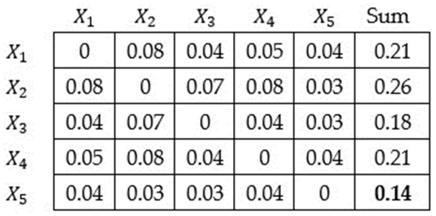Figure 1 collects all the pairwise distances between the data objects of the cluster.

From the matrix in Figure 1, it emerges that the medoid representative of the cluster is the $X_5$ data object, which has a minimal sum (0.14) of the distances to all the other points in the cluster. Moreover, the contribution of the cluster to the function cost $SDM$ is also 0.14.

3.3. Random Swap Algorithm for Sets

The operation of the algorithm is shown in Algorithm 2. With respect to the basic random swap algorithm [11,12], the use of medoids in the refinement Step 4 should be noted.

Due to its ability to search for medoid configurations in the whole data space, random swap is capable of approaching the optimal solution in many practical cases, hopefully, after a small number of iterations $T$.

3.4. Medoids Initialization and Seeding Methods

It has been demonstrated [3,4] that the seeding method for centroids initialization can significantly affect the K-means clustering results. This is likely why the K-sets variant was inferior to the K-swaps algorithm in [8]. It was shown in [4] that significantly better results can be obtained for difficult datasets by using better initialization algorithms such as maximin and K-means++. We, therefore, consider different seeding strategies. We consider the uniform random method, maximin [16], K-means++ [14], and greedy K-means++ [15,17,18].

Uniform: The $K$ medoids are defined by $K$ uniform random selections from the dataset.

Let $X_i$ be a data object and $D\left(X_i\right)$ the minimal distance of $X_i$ from the currently defined centroids.

Maximin: The first medoid is chosen in the dataset by a uniform random selection. Then, maximin chooses the next medoid as a data object with maximal $D\left(X_i\right)$ value. The procedure is continued until all the $K$ medoids have been selected.

K-Means++: This is a randomized variant of the same idea as in maximin; it selects the next medoid by a random switch among the data objects of the dataset, after associating to each data object the probability of being chosen as:

$$\pi \left(X_i\right)=\frac{D{\left(X_i\right)}^2}{{{\displaystyle \sum }}_{j=1}^N{\left(X_j\right)}^2}.$$

Greedy K-Means++: This refines the K-means++ procedure with a sampling step (see Algorithm 3). Except for the first medoid, any new medoid is selected by sampling $S$ candidates from the dataset, and by keeping the one which minimizes the $SDM$ cost function, evaluated according to the currently defined medoids.

Algorithm 3: The Greedy_K-Means++ seeding method

$m_1\leftarrow X_j, j\leftarrow unif\_rand\left(1..N\right)$, $M\leftarrow 1$

$do\{$

$\mathrm{costBest}\leftarrow \infty$

$\mathrm{candBest}\leftarrow ?$

$repeat S times \{$

$\mathrm{select}$ a data object $X^{*}\in X$ with the K-Means++ procedure

$\mathrm{partition}$ $X$ according to $\left\{m_1, m_2,\dots , m_M,X^{*}\right\}$

$\cos \mathrm{t}=SDM()$

$if(\cos \mathrm{t}<\cos \mathrm{tBest}) \{$

$\mathrm{candBest}\leftarrow X^{*}$

$\mathrm{costBest}\leftarrow \cos \mathrm{t}$

$\}$

$\}$

$M\leftarrow M+1$

$m_M\leftarrow \mathrm{candBest}$

$\} while(M<K)$

The value $S$ is a trade-off between the improved seeding and the extra computational due to the $S\ast \left(K-1\right)$ attempts. We fix $S=2+\log K$, as suggested in [17].

The K-medoids Algorithm 1 is used in this work in a repeated way, where a different initialization of the medoids feeds each independent run. As for repeated K-means, the higher the number of repetitions, the higher the chance to achieve a solution “near” to the optimal one.

3.5. Accuracy Clustering Indexes

The proposed new distance functions in Section 3.1 make it possible to qualify the accuracy of a clustering solution achieved by repeated K-medoids or random swaps, by using some well-known internal or external indexes. For benchmark datasets provided of ground truth partition labels (see also later in this paper), the external adjusted rand index ($ARI$) (used in [8]) and the centroid index ($CI$) [12,25,26] can be used to qualify the similarity degree between an obtained solution and the ground truth solution. The $ARI$ index ranges from 0 to 1, with 1 mirroring maximal similarity and 0 expressing the maximal dissimilarity. The $CI$ index ranges from 0 to $K$. A $CI=0$ is a precondition for a clustering solution to be structurally correct, with the found medoids which are very close to the optimal positions. A $CI>0$ indicates the number of medoids which were incorrectly determined.

In addition to the $SDM$ function cost, in this work, the internal Silhouette index ($SI$) [16,27] can be used for checking the degree of separation of the clusters. The $SI$ index ranges from −1 to 1 (see also [12]), with 1 mirroring well-separated clusters. An $SI=0$ indicates high overlapping among clusters. An $SI$ toward −1 characterizes an incorrect clustering.

3.6. Java Implementation

The following gives a flavor of the Java implementation based on parallel streams [12,19,20] of the proposed clustering algorithms for sets. The $dataset$ and $medoids$ are represented by native arrays of $DataObject$ instances. A $DataObject$ holds a set of items (strings) and provides the distance function (either Jaccard or cosine modified distance) and other useful methods for stream management. A $G\_Sets$ class exposes some global parameters such as the dataset dimension $N$, the number of clusters $K$, the number of distinct items $L$, the name and location of the dataset file and so forth.

For generality, the implementation does not rely on the matrix of pairwise distances which is difficult to manage in large datasets. Distances among data objects are, instead, computed on demand and purposely exploit the underlying parallel execution framework.

In Algorithm 4, the $SDM()$ method of $G\_Sets$ is shown. First, a stream is achieved from the dataset, with the $PARALLEL$ parameter which controls whether the stream must be processed in parallel. Then, the stream is open. The intermediate $map$() operation works on the stream by applying a $Function\langle T,R\rangle$ lambda expression to each data object. The lambda receives a $T$ element and returns an $R$ result. In Algorithm 4, $T=R=DataObject$. $map()$ receives a $DataObject dO$ and accumulates in its field $dist$ the sum of distances from $dO$ to every other object in the same cluster (controlled by the CID field of data objects). Then, the modified $dO$ is returned. The terminal $reduce()$ operation adds all the distances held in the data objects and returns a new $DataObject spd$ whose $dist$ contains the required $SDM$.

Algorithm 4: Stream based sum of distances to medoids (SDM) method

public static double SDM() {

Stream<DataObject> pStream =

(PARALLEL) ? Stream.of(dataset).parallel() : Stream.of(dataset);

DataObject sdm = pStream

.map(

dO ->{

int k = dO.getCID(); dO.setDist(0);

for(int i = 0; i<N; ++i) {

if(i! = dO.getID() && dataset[i].getCID() = = k) { //same cluster

dO.setDist(dO.getDist()+dO.distance(dataset[i]));

}

}

return dO;

}

)

.reduce(

new DataObject(),

(d1,d2)->{ DataObject d = new DataObject();

d.setDist(d1.getDist()+d2.getDist()); return d; }

);

return sdm.getDist();

}//SDM

An important issue in the realization in Algorithm 4 is that stream objects can be processed in parallel using the built-in fork/join mechanism [19], which splits the dataset into multiple segments and spawns a separate thread to process the data objects of a same segment. The various results are finally combined, in parallel, by the $reduce()$ operation which returns a new $DataObject$ $sdm$ containing the overall sum of distances.

The correctness and actual efficiency of the Java code in Algorithm 4 rests on the designer, which must absolutely avoid modifications of shared objects during the parallel execution of the lambda expressions. For example, the lambda of each $map()$ operation in Algorithm 4 purposely modifies only the received $dO$ parameter object; thus, data interferences are completely avoided.

The stream-based programming style shown in Algorithm 4 was also adopted in the implementation of K-medoids, random swap, and in all the operations which can benefit from a parallel execution.

Algorithm 5 shows an excerpt of the stream-based K-medoids algorithm.

Algorithm 5: An excerpt of the K-Medoids algorithm in Java

…

//clusters’ queues for saving belonging data objects

ConcurrentLinkedQueue<DataObject>[] clusters = new ConcurrentLinkedQueue[K];

for(int c = 0; c<K; ++c) clusters[c] = new ConcurrentLinkedQueue<>();

…

seeding(INIT_METHOD); //initialize medoids

do{

for(int c = 0; c<K; ++c) clusters[c].clear();

//partitioning step: assign data objects to clusters

Stream<DataObject> do_stream = Stream.of(dataset);

if(PARALLEL) do_stream = do_stream.parallel();

do_stream

.map(dO -> {

double md = Double.MAX_VALUE;

for(int k = 0; k<K; ++k) {

double d = dO.distance(medoids[k]);

if(d<md) { md = d; dO.setCID(k); }

}

clusters[ dO.getCID() ].add(dO); //add data object dO to its partition cluster

return dO;

})

.forEach(dO->{}); //only to trigger the map operation

//update medoids step

for(int h = 0; h<K; ++h) {

Stream<DataObject> c_stream = clusters[h].stream(); //open stream on cluster[h]

if(PARALLEL) c_stream = c_stream.parallel();

final int H = h; //turn h into an effective final variable H

DataObject neutral = new DataObject(); neutral.setDist(Double.MAX_VALUE);

DataObject best = c_stream

.map(dO->{

double c = 0D;

for(DataObject q: clusters[H]) { if(q! = dO) c = c+ dO.distance(q); }

dO.setDist(c); //save the distance sum to other objects of the cluster

return dO;

})

.reduce(neutral, (d1,d2)->{ if(d1.getDist()<d2.getDist()) return d1; return d2; });

newMedoids[h] = new DataObject(best); newMedoids[h].setN(clusters[h].size());

}//for(int h = 0;…

…

}while(!termination());

…

In the partitioning step (see also Algorithm 1), the nearest medoid to each data object is determined and the label of the medoid (its index) is assigned to the data object. As part of the $map()$ operation, references of all the objects which belong to the same cluster are collected into distinct partition lists, to be used in the second step of medoids update. A critical issue concerns the modification of a shared partition list. To avoid data race conditions, partition lists are purposely realized as $ConcurrentLinkedQueue$ lists which are totally lock free and can be safely accessed simultaneously by multiple threads.

Partition lists can be processed in parallel in the update medoids step. As shown in Algorithm 5, for each data object $dO$ of a cluster, first, the sum of distances from $dO$ to all the remaining objects of the same cluster is accumulated in $dO$ as part of a $map()$ operation. Then, a $reduce()$ operation is used which identifies and returns the data object ($best$) which has a minimal sum of distances to the other objects of the same cluster.

In Algorithm 5, new medoids are temporarily defined and are compared with current medoids in the $termination()$ method, which checks termination (by convergence or by maximum number of executed iterations) and, finally, makes new medoids current medoids for the next iteration.

4. Experimental Setup

We use the 15 artificial datasets described in [8] for testing the algorithms. They are all available in [22]. All datasets have N = 1200 data objects and vary in the size $L$ of the vocabulary of elementary items, the number $K$ of clusters, the overlapping percentage $o$, and the type $t$ which specifies how balanced are the cluster sizes. The value $t=1$ denotes to equal cluster sizes. The datasets are named accordingly as data_N_L_K_o_t, see

Table 1. Synthetic datasets for clustering sets.

Dataset	Type	4 Big	12 Small
data_1200_100_16_5_1	1	75	75
data_1200_200_4_5_1	2	120	60
data_1200_200_8_5_1	3	150	50
data_1200_200_16_0_1	4	187–188	37–38
data_1200_200_16_5_1	5	210	30
data_1200_200_16_5_2
data_1200_200_16_5_3
data_1200_200_16_5_4
data_1200_200_16_5_5
data_1200_200_16_10_1
data_1200_200_16_20_1
data_1200_200_16_40_1
data_1200_200_32_5_1
data_1200_400_16_5_1
data_1200_800_16_5_1

.

Ground truth partitions are provided to measure the accuracy by the adjusted rand index ($ARI$) and the centroid index ($CI$) [25,26] of a found clustering solution.

We cluster each dataset by repeated K-medoids using 1000 runs. For the initialization, we use uniform random, maximin, K-means++, and the greedy-K-means++ (G-K-means++) seeding.

The following quantities were observed: The best value of the sum of distances to medoids function cost $SDM$ (indicated as $bSDM$) emerged from the various runs, and the corresponding $ARI$ ($bARI$), $CI$ ($bCI$), and $Silhouette$ ($bSI$) indexes. In addition, the $Success Rate$ ($SR$), that is the number of runs that terminated with a $CI=0$, the average $ARI$ ($aARI$), and the average $CI$ ($aCI$) estimated in the 1000 runs, were also registered.

5. Clustering Results

The effects of the seeding methods were preliminarily studied using the $data\_1200\_100\_16\_5\_1$ dataset (see Table 1). The results are reported in

Table 2. Results of repeated K-medoids (1000 runs) under different seeding methods, on the $data\_1200\_100\_16\_5\_1$ dataset with weighted Jaccard distance.

Seeding	bSDM	bARI	bCI	SR	bSI	aARI	aCI
Uniform Random	1513	0.99	0	6.0%	0.71	0.72	2.71
Maximin	1513	0.99	0	17.5%	0.71	0.89	1.14
K-Means++	1513	0.99	0	14.5%	0.71	0.86	1.50
G-K-Means++	1513	0.99	0	39.6%	0.71	0.93	0.69

.

Simulation experiments were carried out on a Win11 Pro, Dell XPS 8940, Intel i7–10700 (8 physical cores), [email protected] GHz, 32 GB Ram, and Java 17.

As one can see from Table 2, all the four seeding methods agree on the best $SDM$, $ARI$, $CI,$ and SI. However, they significantly differ in the $success rate$ and the average $ARI$ and the average $CI$.

The best results follow from the careful seeding ensured by G-K-means++ where a $success rate$ of about 40%, an average $ARI$ of 0.93, and an average $CI$ of about 0.69 were observed, although with an increased computational time. Table 2 also confirms that maximin, after G-K-means++, is capable of offering better results than uniform random or K-means++ seeding. The Silhouette index ($SI$) mirrors the limited overlapping percentage ($o=5\%$) present in the dataset.

The dataset $data\_1200\_100\_16\_5\_1$ was also studied by using the parallel version of the implemented random swap algorithm ($PRS$) (see Algorithm 2) separately fed by each one of the four seeding methods. At most, 100 swap iterations were set. The minimal number of swaps required to detect the “best” solution (minimal $SDM$ cost) and corresponding $ARI$, $CI$, and $SI$ indexes are reported in

Table 3. Results of parallel random swap (max 100 iterations) under different seeding methods, on the $data\_1200\_100\_16\_5\_1$ dataset with weighted Jaccard distance.

Seeding	SDM	ARI	CI	SI	Iterations
Uniform random	1513	0.99	0	0.71	26
Maximin	1513	0.99	0	0.71	4
K-means++	1513	0.99	0	0.71	18
G-K-means++	1513	0.99	0	0.71	4

.

From Table 3 it emerges that even with the uniform random seeding, $PRS$ was able to find the best solution with few iterations.

The effect of seeding methods on the $data\_1200\_100\_16\_5\_1$ dataset was also observed with the other datasets. Therefore, in the following, for simplicity, only the results gathered by using repeated K-medoids and parallel random swap when seeded, respectively, by uniform random and by G-K-means++ are reported in

Table 4. Results of repeated K-medoids (1000 runs) with uniform random seeding on the datasets of Table 1 with weighted Jaccard distance.

Dataset	bSDM	bARI	bCI	SR	bSI	aARI	aCI
data_1200_100_16_5_1	1513	0.99	0	6.0%	0.71	0.72	2.71
data_1200_200_4_5_1	7986	1.0	0	85.5%	0.89	0.94	0.15
data_1200_200_8_5_1	4827	0.99	0	41.5%	0.79	0.86	0.74
data_1200_200_16_0_1	1419	1.0	0	2.2%	0.83	0.83	2.21
data_1200_200_16_5_1	3124	0.99	0	7.5%	0.68	0.72	2.68
data_1200_200_16_5_2	3320	0.99	0	5.1%	0.69	0.73	2.91
data_1200_200_16_5_3	3434	0.99	0	1.8%	0.70	0.77	3.24
data_1200_200_16_5_4	4110	0.98	0	0.6%	0.72	0.77	3.91
data_1200_200_16_5_5	5111	0.99	0	0.4%	0.72	0.79	3.62
data_1200_200_16_10_1	3262	0.99	0	4.1%	0.67	0.65	3.14
data_1200_200_16_20_1	3472	0.99	0	1.9%	0.64	0.56	3.54
data_1200_200_16_40_1	4628	0.89	1	0.0%	0.50	0.41	3.86
data_1200_200_32_5_1	2136	0.94	1	0.0%	0.55	0.54	7.32
data_1200_400_16_5_1	6016	1.0	0	8.8%	0.68	0.70	2.72
data_1200_800_16_5_1	10,285	0.99	0	21.8%	0.66	0.79	1.96

,

Table 5. Results of repeated K-medoids (1000 runs) with G-K-means++ seeding, on the datasets of Table 1 with weighted Jaccard distance.

Dataset	bSDM	bARI	bCI	SR	bSI	aARI	aCI
data_1200_100_16_5_1	1513	0.99	0	39.6%	0.71	0.93	0.69
data_1200_200_4_5_1	7986	1.0	0	99.1%	0.89	1.0	0.01
data_1200_200_8_5_1	4827	0.99	0	78.0%	0.79	0.95	0.22
data_1200_200_16_0_1	1419	1.0	0	45.5%	0.83	0.95	0.58
data_1200_200_16_5_1	3124	0.99	0	30.0%	0.68	0.91	0.88
data_1200_200_16_5_2	3320	0.99	0	31.7%	0.69	0.93	0.87
data_1200_200_16_5_3	3434	0.99	0	20.1%	0.70	0.93	1.10
data_1200_200_16_5_4	4110	0.98	0	12.9%	0.72	0.93	1.34
data_1200_200_16_5_5	4926	0.99	0	10.5%	0.72	0.91	1.47
data_1200_200_16_10_1	3262	0.99	0	21.5%	0.67	0.90	0.94
data_1200_200_16_20_1	3472	0.99	0	31.2%	0.64	0.89	0.93
data_1200_200_16_40_1	3460	0.99	0	13.0%	0.59	0.78	1.48
data_1200_200_32_5_1	1824	1.0	0	9.8%	0.59	0.90	1.73
data_1200_400_16_5_1	6016	1.0	0	43.0%	0.68	0.93	0.68
data_1200_800_16_5_1	10,285	0.99	0	59.0%	0.66	0.95	0.44

,

Table 6. Results of parallel random swap (max 100 iterations) with uniform random seeding, on the datasets of Table 1 with weighted Jaccard distance.

Dataset	SDM	ARI	CI	SI	Iterations
data_1200_100_16_5_1	1513	0.99	0	0.71	26
data_1200_200_4_5_1	7986	1.0	0	0.89	5
data_1200_200_8_5_1	4825	0.99	0	0.79	51
data_1200_200_16_0_1	1419	1.0	0	0.83	2
data_1200_200_16_5_1	3124	0.99	0	0.68	10
data_1200_200_16_5_2	3320	0.99	0	0.69	16
data_1200_200_16_5_3	3434	0.99	0	0.70	42
data_1200_200_16_5_4	4202	0.98	0	0.72	27
data_1200_200_16_5_5	5000	0.99	0	0.72	99
data_1200_200_16_10_1	3262	0.99	0	0.67	60
data_1200_200_16_20_1	3480	0.99	0	0.64	14
data_1200_200_16_40_1	3467	0.99	0	0.59	63
data_1200_200_32_5_1	1825	0.99	0	0.59	85
data_1200_400_16_5_1	6016	1.0	0	0.68	13
data_1200_800_16_5_1	10287	0.99	0	0.66	9

and

Table 7. Results of parallel random swap (max 100 iterations) with G-K-means++ seeding, on the datasets of Table 1 with weighted Jaccard distance.

Dataset	SDM	ARI	CI	SI	Iterations
data_1200_100_16_5_1	1513	0.99	0	0.71	2
data_1200_200_4_5_1	7986	1.0	0	0.89	2
data_1200_200_8_5_1	4827	0.99	0	0.79	1
data_1200_200_16_0_1	1419	1.0	0	0.83	2
data_1200_200_16_5_1	3126	0.99	0	0.68	1
data_1200_200_16_5_2	3320	0.99	0	0.69	6
data_1200_200_16_5_3	3436	0.99	0	0.70	24
data_1200_200_16_5_4	4202	0.98	0	0.72	15
data_1200_200_16_5_5	5000	0.99	0	0.72	4
data_1200_200_16_10_1	3266	0.99	0	0.67	6
data_1200_200_16_20_1	3472	0.99	0	0.64	4
data_1200_200_16_40_1	3460	0.99	0	0.59	10
data_1200_200_32_5_1	1825	0.99	0	0.59	43
data_1200_400_16_5_1	6016	1.0	0	0.68	2
data_1200_800_16_5_1	10285	0.99	0	0.66	2

.

From the results in Table 4 and Table 5, it emerges that for almost all the datasets, 1000 repetitions of K-medoids with uniform random seeding are sufficient for obtaining a good clustering solution. However, the use of G-K-means++ seeding not only enables a very good solution to be achieved in all the cases, as reflected by the values of the $ARI$, $CI$, and $SI$ indexes, but it also increases significantly the $Success Rate$.

Only for the two datasets $data\_1200\_200\_16\_40\_1$ and $data\_1200\_200\_32\_5\_1$, 1000 repetitions of K-medoids with uniform random seeding proved to be insufficient for generating a solution with minimal $SDM$, highest $ARI,$ and $CI=0$. This is due to the combination of design factors of the datasets, i.e., the number of clusters and the overlapping degree.

By increasing the number of runs to 10⁴, both the datasets were correctly handled by K-medoids with uniform random seeding, with a resultant solution for $data\_1200\_200\_16\_40\_1$ which has minimal SDM = 3460, $ARI=0.99$, $CI=0,$ and $SI=0.58$, and an average $ARI=0.45$, average $CI=3.85,$ and $Success Rate=8\times {10}^{-4}$.

For the dataset $data\_1200\_400\_16\_5\_1$, the emerged best solution has minimal SDM = 1824, $ARI=1.0$, CI = 0, $SI=0.59$, and average $ARI=0.53$, average $CI=7.34,$ and $Success Rate=7\times {10}^{-4}$.

The benefits of careful seeding are confirmed by all the results shown in Table 5.

The results in Table 6 and Table 7 are the average of 10 repetitions of the parallel random swap ($PRS$) algorithm. As one can see, the collected data agree with the results achieved by repeated K-medoids under the same seeding method. $PRS$, though, was able to solve the clustering problem ($CI=0$) even under the uniform random initialization of medoids. In addition, using G-K-means++ significantly reduces the number of iterations the clustering solution requires to stabilize.

Separate experiments were executed by using the modified Otsuka–Ochiai cosine distance. Except for the exact $SDM$ values, which clearly depend on the specific distance measure adopted, the bARI, $bCI$, and $bSI$ results are identical to the case the modified Jaccard distance was adopted, especially when the G-K-means++ seeding is used. Therefore, such results are not reported for brevity.

For comparison purposes with the results documented in [8] and achieved by using K-sets and K-swaps,

Table 8. $ARI$ vs. the number of clusters $K$.

Algorithm	K = 4	K = 8	K = 16	K = 32	Average
K-medoidsGKM++	1.0	0.99	0.99	1.0	1.0
PRSGKM++	1.0	0.99	0.99	0.99	0.99
K-sets	1.0	1.0	0.92	0.88	0.95
K-swaps	1.0	1.0	1.0	0.99	1.0

collects the achieved clustering results when the number of clusters $K$ varies from 4 to 32;

Table 9. $ARI$ vs. the resolution $L$.

Algorithm	L = 100	L = 200	L = 400	L = 800	Average
K-medoidsGKM++	0.99	0.99	1.0	0.99	0.99
PRSGKM++	0.99	0.99	1.0	0.99	0.99
K-sets	0.91	0.92	0.92	0.93	0.92
K-swaps	0.99	1.0	0.99	0.99	0.99

shows the results when the resolution $L$ varies from 100 to 800;

Table 10. $ARI$ vs. the overlapping level $o$.

Algorithm	o = 0%	o = 5%	o = 10%	o = 20%	o = 40%	Average
K-medoidsGKM++	1.0	0.99	0.99	0.99	0.99	0.99
PRSGKM++	1.0	0.99	0.99	0.99	0.99	0.99
K-sets	0.86	0.92	0.86	0.91	0.92	0.89
K-swaps	1.0	1.0	0.99	0.99	0.99	0.99

reports the emerged data when the overlapping level $o$ of clusters varies from 0% to 40%; and finally,

Table 11. $ARI$ vs. the cluster types $t$.

Algorithm	t = 1	t = 2	t = 3	t = 4	t = 5	Average
K-medoidsGKM++	0.99	0.99	0.99	0.98	0.99	0.99
PRSGKM++	0.99	0.99	0.99	0.98	0.99	0.99
K-sets	0.92	0.86	0.80	0.85	0.85	0.86
K-swaps	1.0	0.99	0.99	1.0	0.99	0.99

illustrates the results when the type of clusters $t$ is varied from 1 to 5.

The table results were confirmed by K-medoids and parallel random swap ($PRS$) under G-K-means++ seeding (GKM++).

Since in [8] the $CI$ and $SI$ indexes were not reported, the table results show only the best-achieved $ARI$ and the average $ARI$ calculated along the values in a table row.

In light of the data shown in Table 8, Table 9, Table 10 and Table 11, the algorithms proposed in this paper for clustering sets are capable of generating solutions with the same accuracy as the approach described in [8], and in some cases can deliver better performance.

Time Efficiency

The time complexity of the implemented K-medoids algorithm is $O\left(N^{2}KTl\right)$, where $N$ is the number of the data objects (sets) of the dataset, $K$ is the number of medoids, $T$ is the number of iterations, and $l$ is the average length of a set.

In the following, some information is provided to determine the time computational benefits that can be gathered from using Java parallel streams. The experimental results reported in Table 4, Table 5, Table 6, Table 7, Table 8, Table 9, Table 10 and Table 11 were all achieved by executing the proposed K-medoids or random swap algorithms in parallel (parameter $PARALLEL=true$).

Table 12. Results of 2000 repetitions of K-medoids^G-K-Means++ with weighted Jaccard distance on the data_1200_200_32_5_1 dataset (8 physical cores).

Execution Mode	$\mathit{S}\mathit{D}\mathit{M}$	$\mathit{A}\mathit{R}\mathit{I}$	$\mathit{C}\mathit{I}$	$\mathit{S}\mathit{R}$	$\mathit{E}\mathit{T} \left(\mathbf{msec}\right)$	$\mathit{I}\mathit{T}$	$\mathit{a}\mathit{E}{\mathit{T}}^{\mathit{i}} \left(\mathbf{msec}\right)$
Sequential	1824	1.0	0	8.9%	4,425,118	10,551	442
Parallel	1824	1.0	0	9.8%	639,585	10,872	63

reports the results of 2000 repetitions of K-medoids, with G-K-means++ seeding and modified Jaccard distance, on the data_1200_200_32_5_1 dataset, separately, in sequential, and in parallel mode. The elapsed time $ET$(in msec) and the total number of completed iterations ($IT$) were also measured. Then, the average elapsed time per iteration, $aE{T}^i=\frac{ET}{IT}$, was computed.

Then, the speedup was estimated as follows:

$$speedup=\frac{Sequential\left(aE{T}^i\right)}{Parallel\left(aE{T}^i\right)}.$$

From the results in Table 12, we can calculate a speedup of 442/63 = 7.02. This corresponds to a parallel efficiency (eight physical cores) of 7.02/8 = 87.8%.

Note that the clustering algorithm executes the same computational steps in sequential and parallel modes. Despite the small value of the dataset size, and then of the clusters’ size, the speedup value reflects a good exploitation of the parallelism in the partitioning and the medoids update steps of K-medoids (see Algorithm 1), as well as in the recurrent calculations of the $SDM$ and of the Silhouette clustering index $SI$.

6. Conclusions

This paper proposes a novel approach to clustering variable-sized sets of elementary items. An example of such data occurs in medical applications where patient diagnoses can be clustered to help discover a patient’s risk of contracting a future illness due to its similarity with other patients.

The new approach is based on medoids. Two algorithms (K-medoids and random swap) were implemented to work with the well-known Jaccard or Otsula–Ochiai cosine distance measures adjusted to exploit some application-sensitive information concerning the global frequency of elementary items in the dataset.

The proposal makes it possible to compute the distance between any pair of sets or data objects. This enables the centroid/medoid of a cluster to be any data object of the dataset. This differs from the inspiring work by [8], where the representative of a cluster is a histogram of the uses of the items in the cluster, and a distance measure is introduced between a data object and the cluster histogram.

The new approach proves to be effective in generating reliable clustering solutions. In addition, an efficient implementation in Java based on parallel streams [12,19,20] was realized to cope with the $O\left(N^2\right)$ computational cost related to computing the all pairwise distances in K-medoids and in the evaluation of some clustering accuracy indexes.

This paper demonstrates the benefits of the proposed approach by applying it to 15 synthetic datasets [22] which were also used in [8]. The experimental results confirm the achievement of high-quality clustering solutions, which can outperform the results reported in [8].

Future research aims at improving the Java implementation of the algorithms; applying the algorithms to realistic datasets such as clustering healthcare records as in [8]; and exploiting the approach in other clustering methods. In addition, considering the problems discussed in [28] about weaknesses of medoids when averaging GPS trajectories, which in general can also be problems in clustering sets, another future issue of this work will concern a possible replacement of medoids by some specific definition of the mean of the data objects of a cluster.