
An Alternative Multi-Physics-Based Methodology for Strongly Coupled Electro-Magneto-Mechanical Problems

 ,
, 
Abstract
1. Introduction
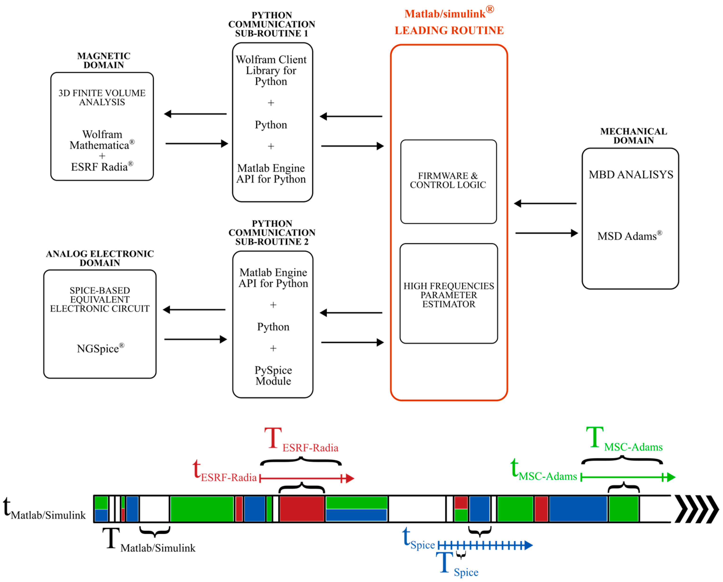
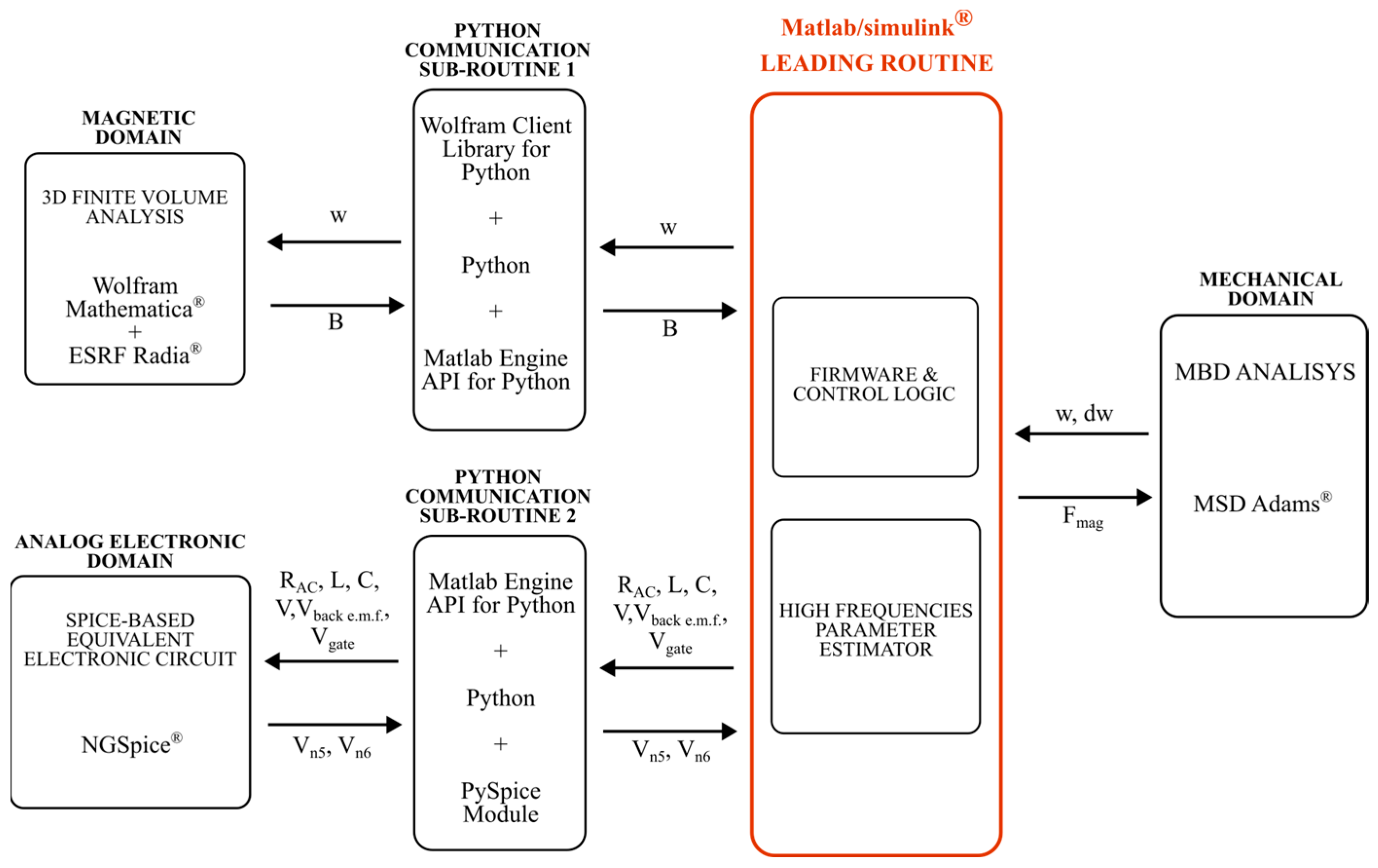
2. The Proposed Multi-Domain Architecture
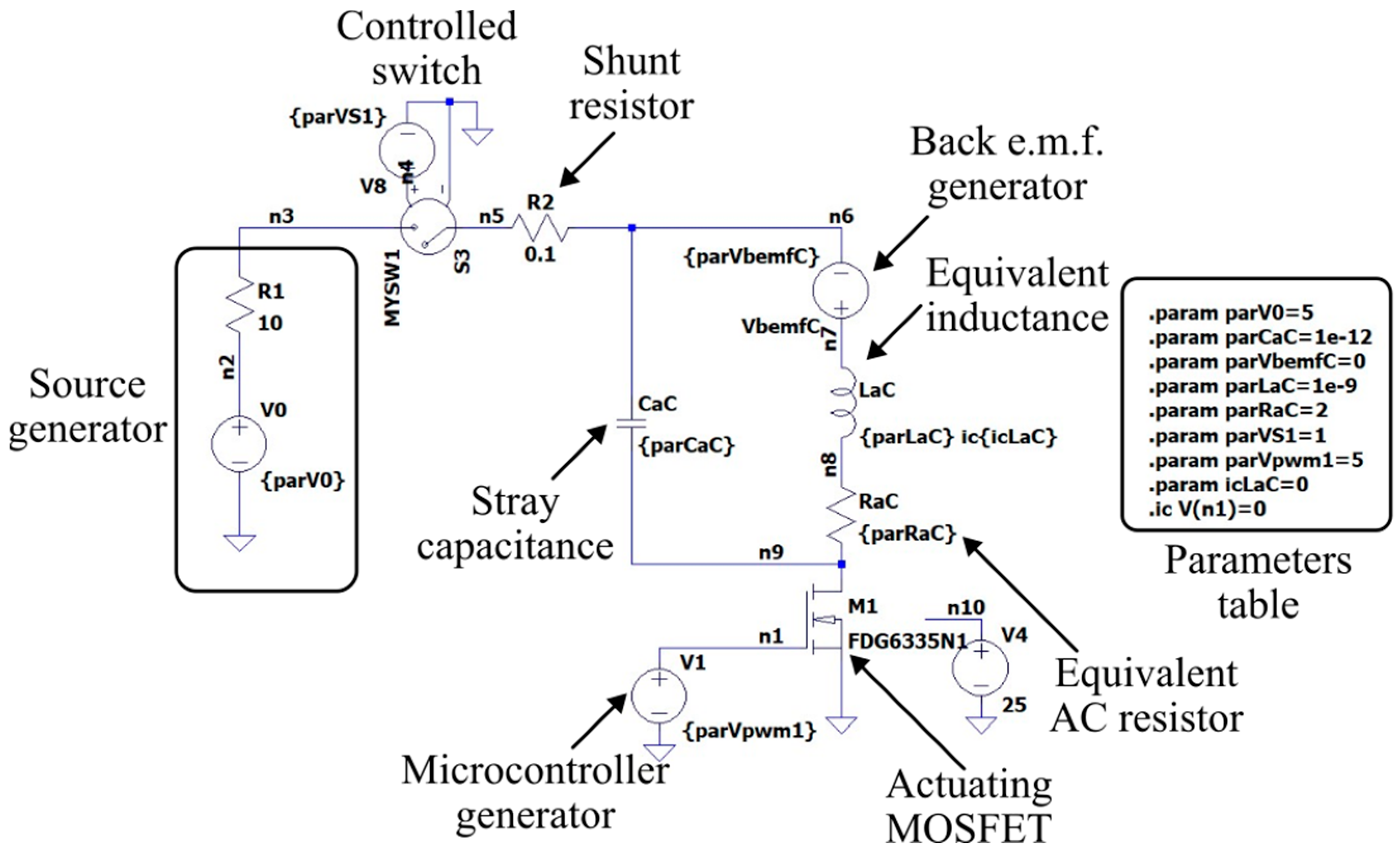
3. Spice-Based Analog Electronic Domain Integration
3.1. Introduction
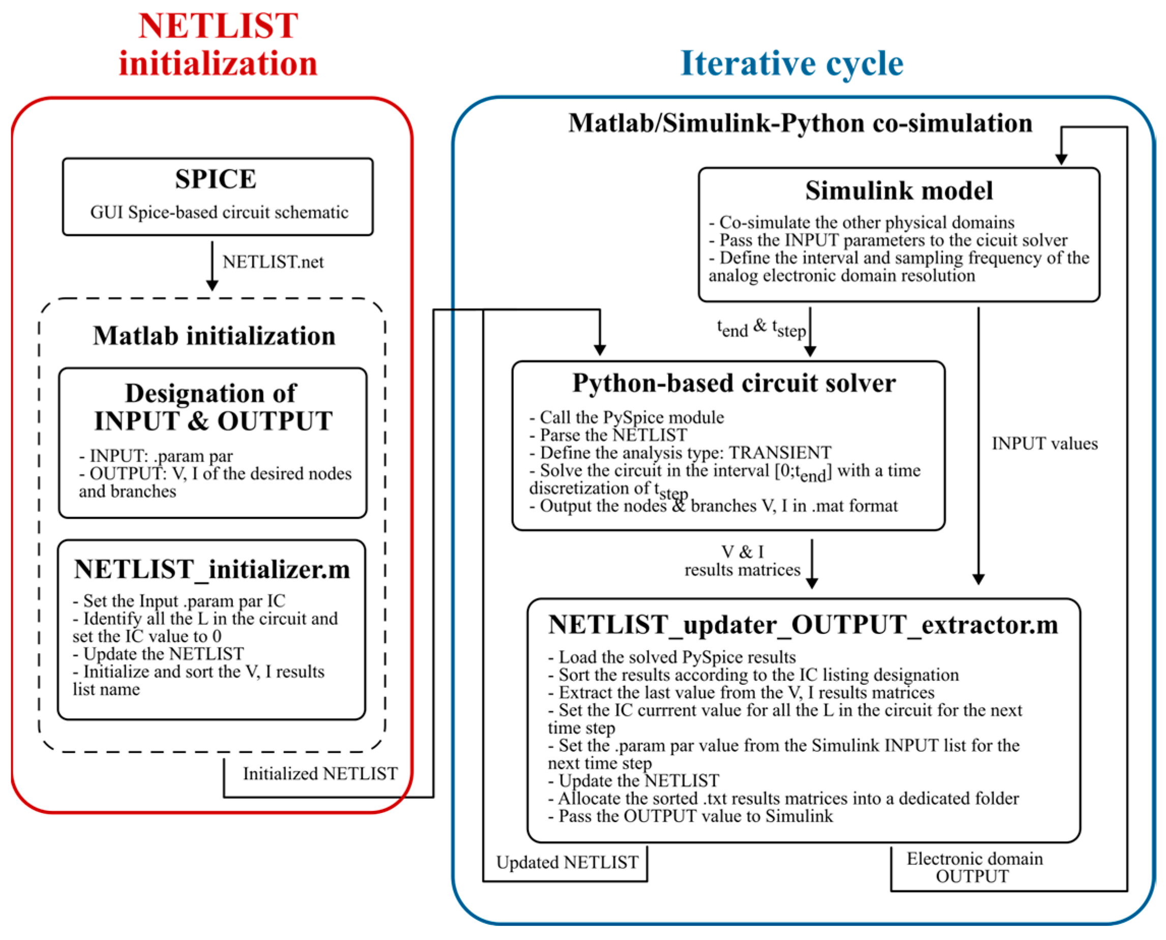
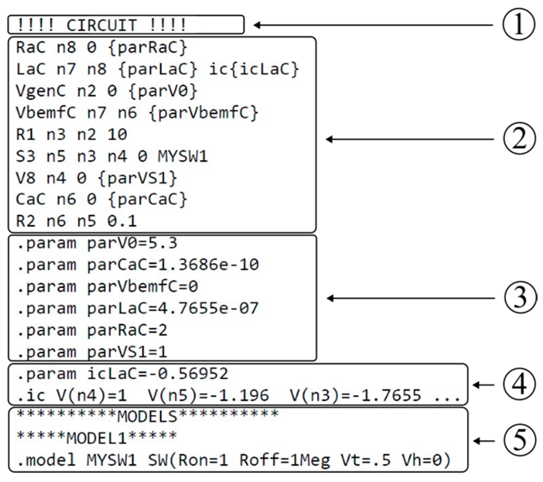
3.2. The Proposed Spice-Based Co-Simulation Algorithm
4. ESRF Radia-Based Magnetostatic Domain Integration
4.1. Introduction
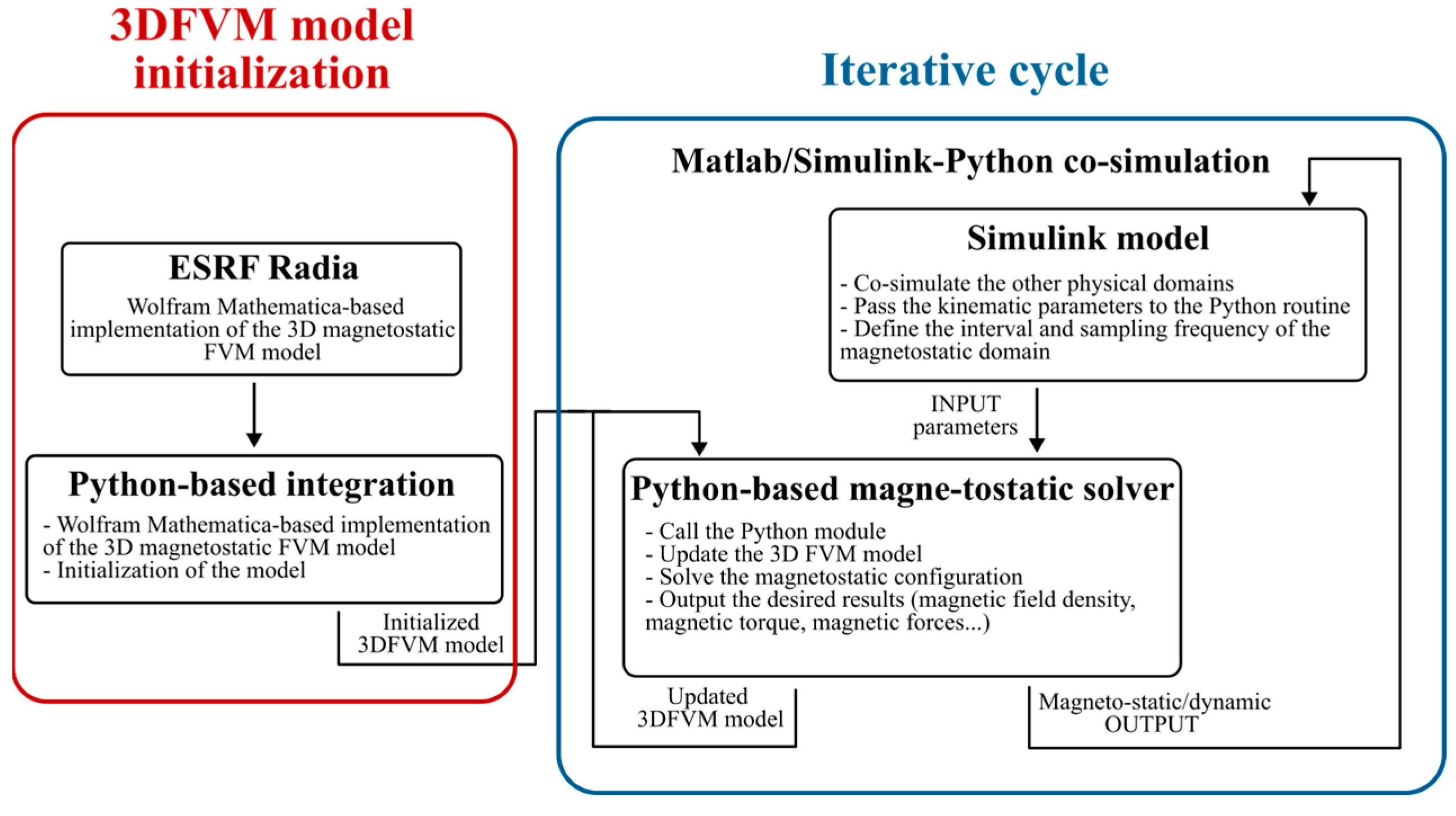
4.2. The Proposed ESRF Radia-Based Co-Simulation Algorithm
5. The Case Study
5.1. Introduction
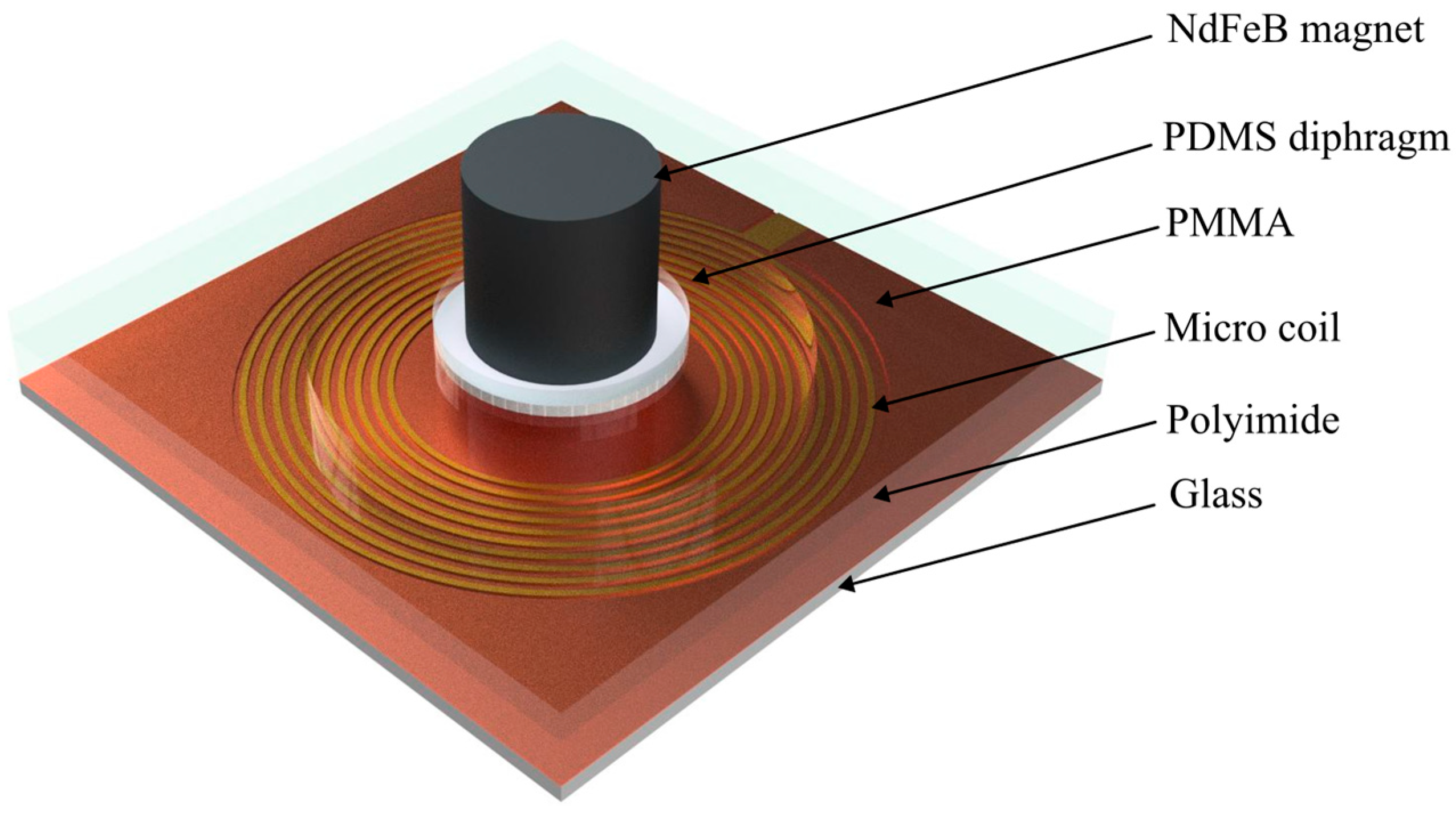
5.2. The Device
5.3. The Governing Equations
5.3.1. The Planar Micro-Coil Characterization
- is the porosity factor of the material.
- is the equivalent thickness of the material and for a round wire and is equal to , where is the diameter of the wire.
- is the skin dept in the wire.
- is the number of turns per layer.
- is the number of Litz wire, which is 1 for round wire.
- is the height of the core window.
- is the resistivity of the wire material.
- is the permeability constant equal to .
- is the principal operating frequency.
- is the equivalent number of layers.
5.3.2. The PDMS Diaphragm Characterization
5.4. The Multi-Domain Model
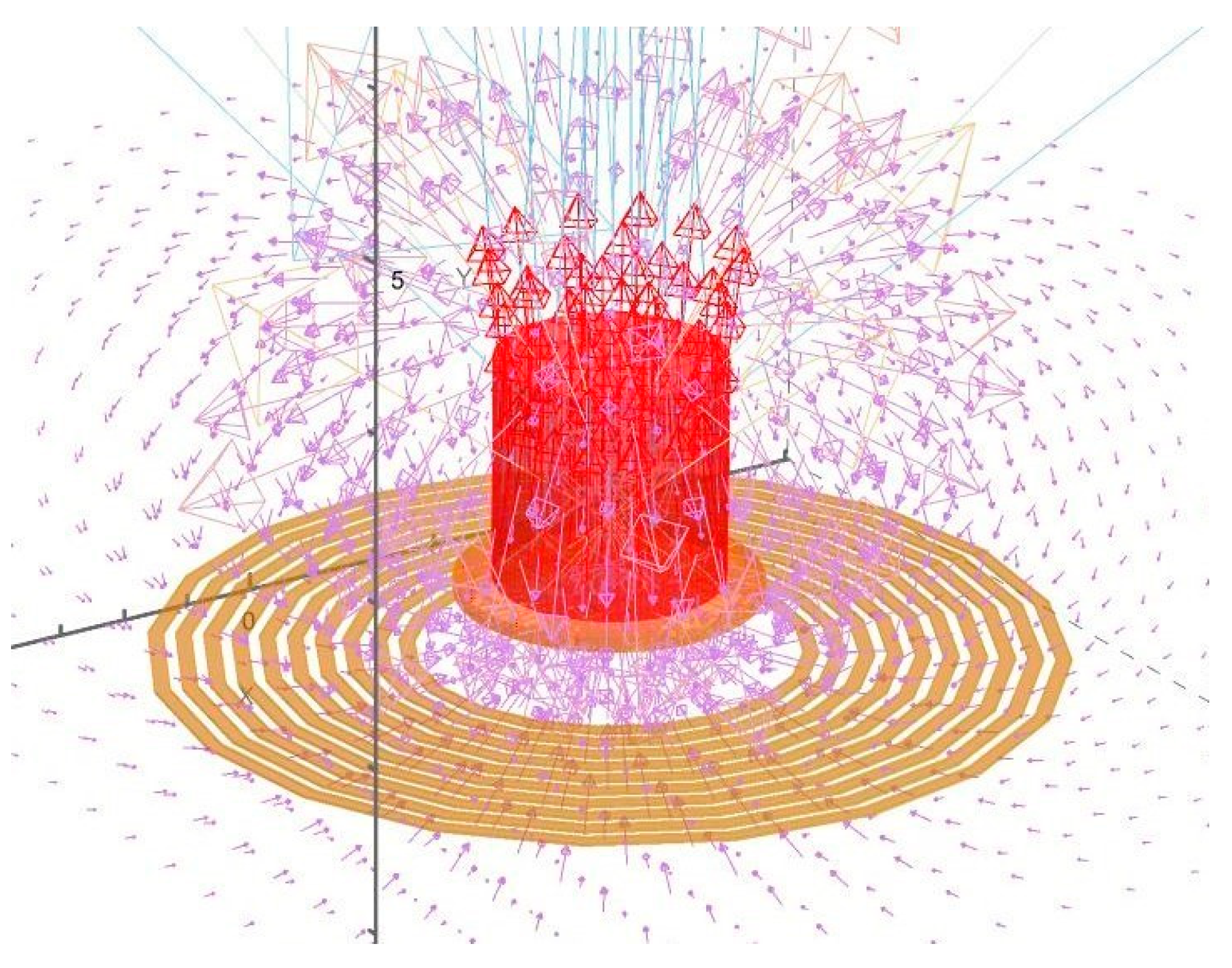
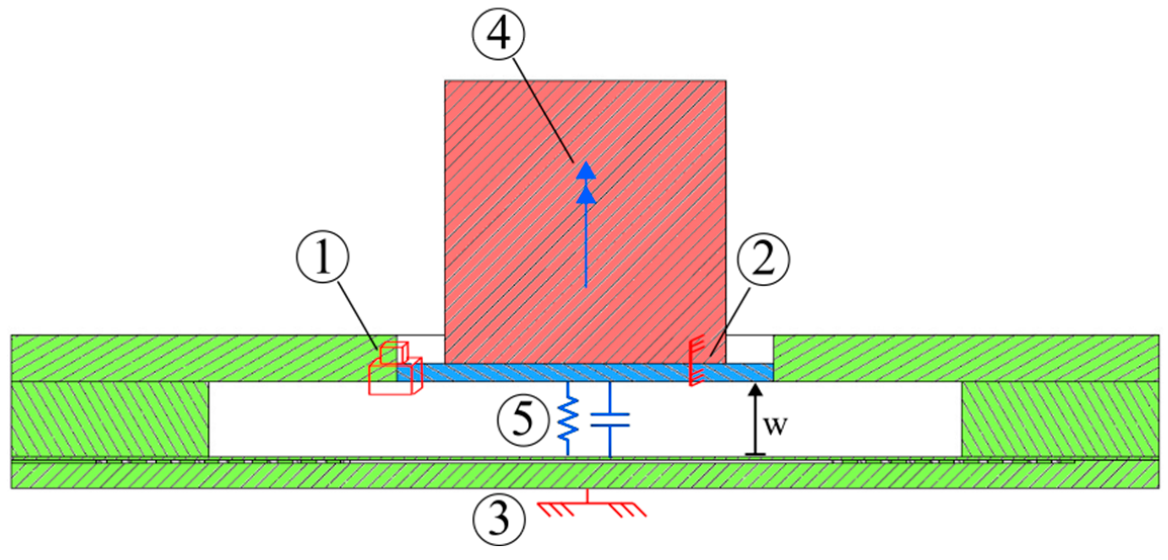
- The NdFeB permanent magnet (red body);
- The PDMS diaphragm (blue body);
- The frame (green body) was composed by the PMMA plate, the micro-coil, the polyimide, and the glass substrate.
- The kinematic deformation properties of the membrane were modeled through a prismatic joint ➀ between the fictitious diaphragm disk and the frame.
- The magnet was kinematically constrained through a fixed joint ➁ to the fictitious membrane.
- A fixed constraint ➂ settled the frame to the ground.
- A magnetic force ➃ was applied between the magnet and the frame. Its absolute value and the verse of application represented one of the co-simulation state variables exchanged among the different simulation platforms.
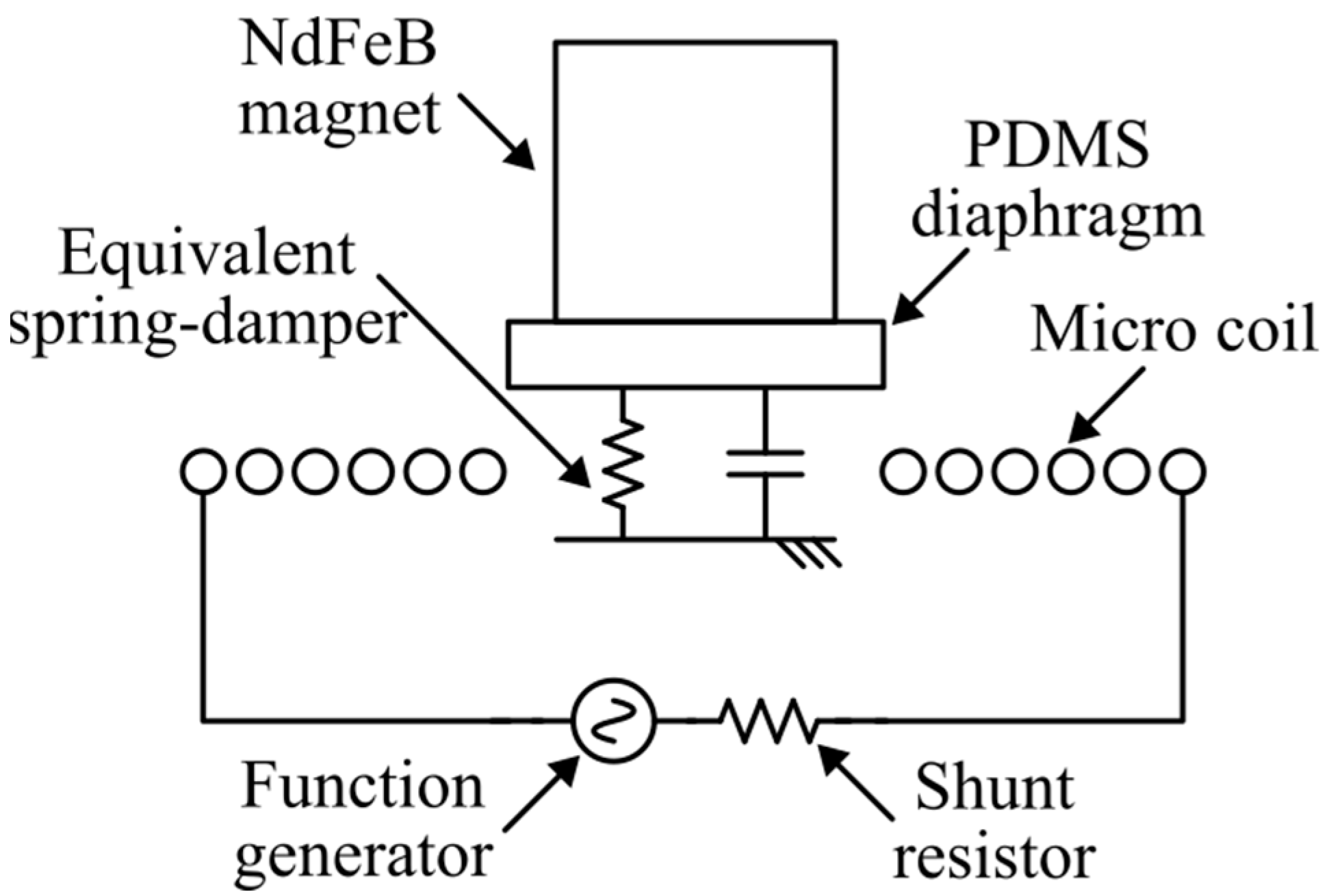
- A spring-damper equivalent force ➄ was added to replicate the elastic and dissipative properties of the PDMS diaphragm. The constitutive parameters values were estimated according to Equations (12)–(15).
- The measure and of the equivalent deflection was measured between the frame and the disk and was passed back to the leading routine as presented in Figure 6 to compute the induced e.m.f.
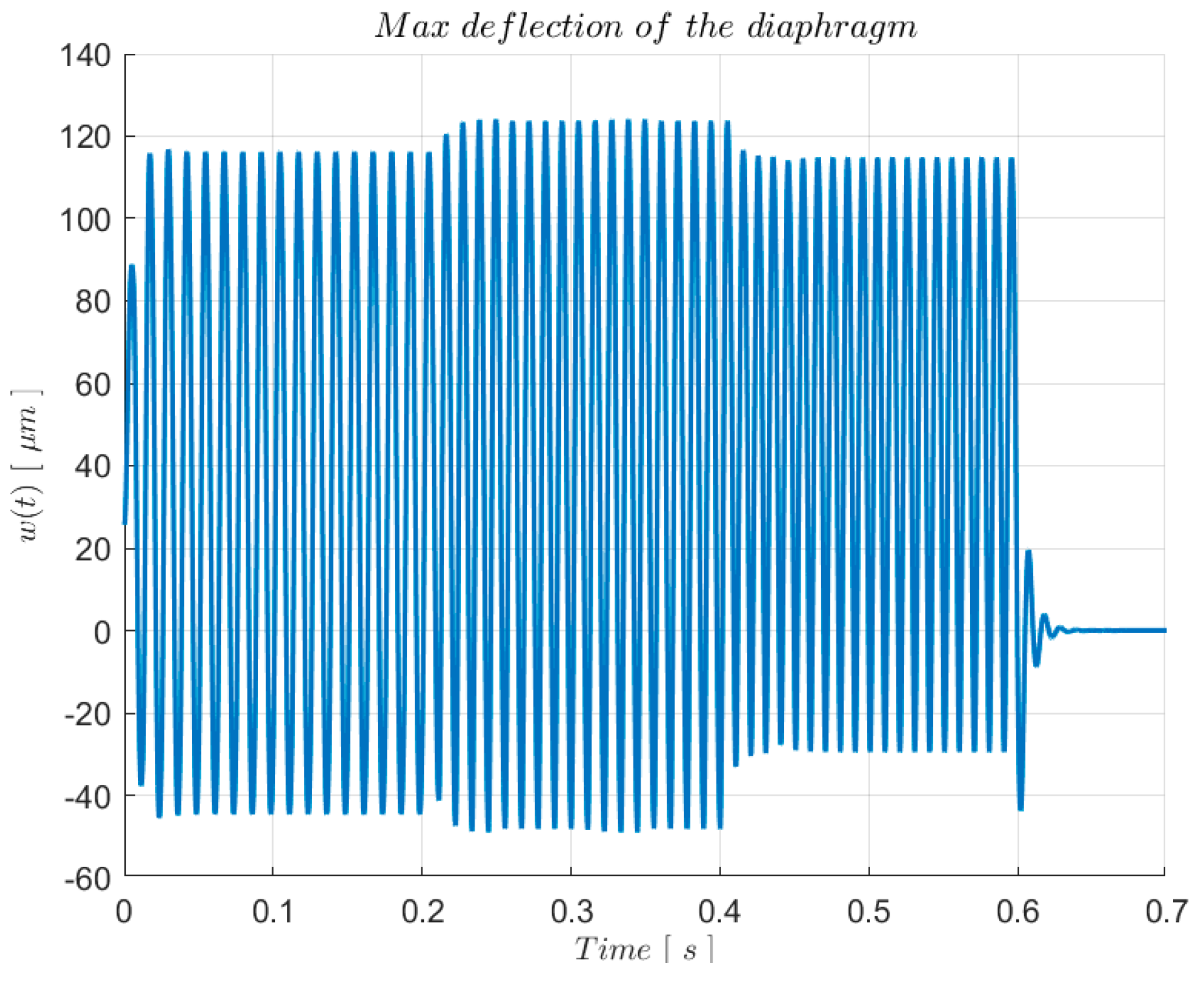
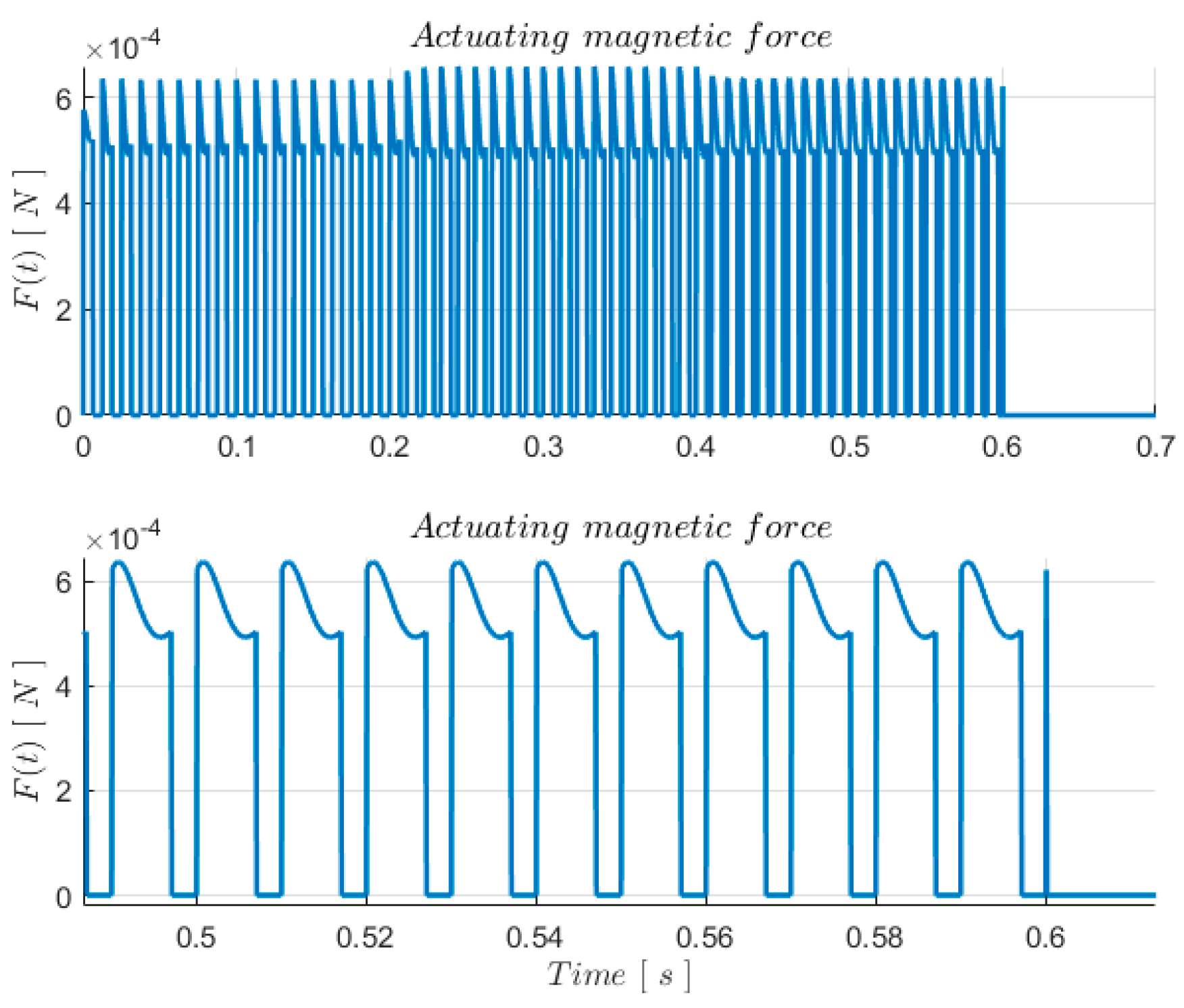
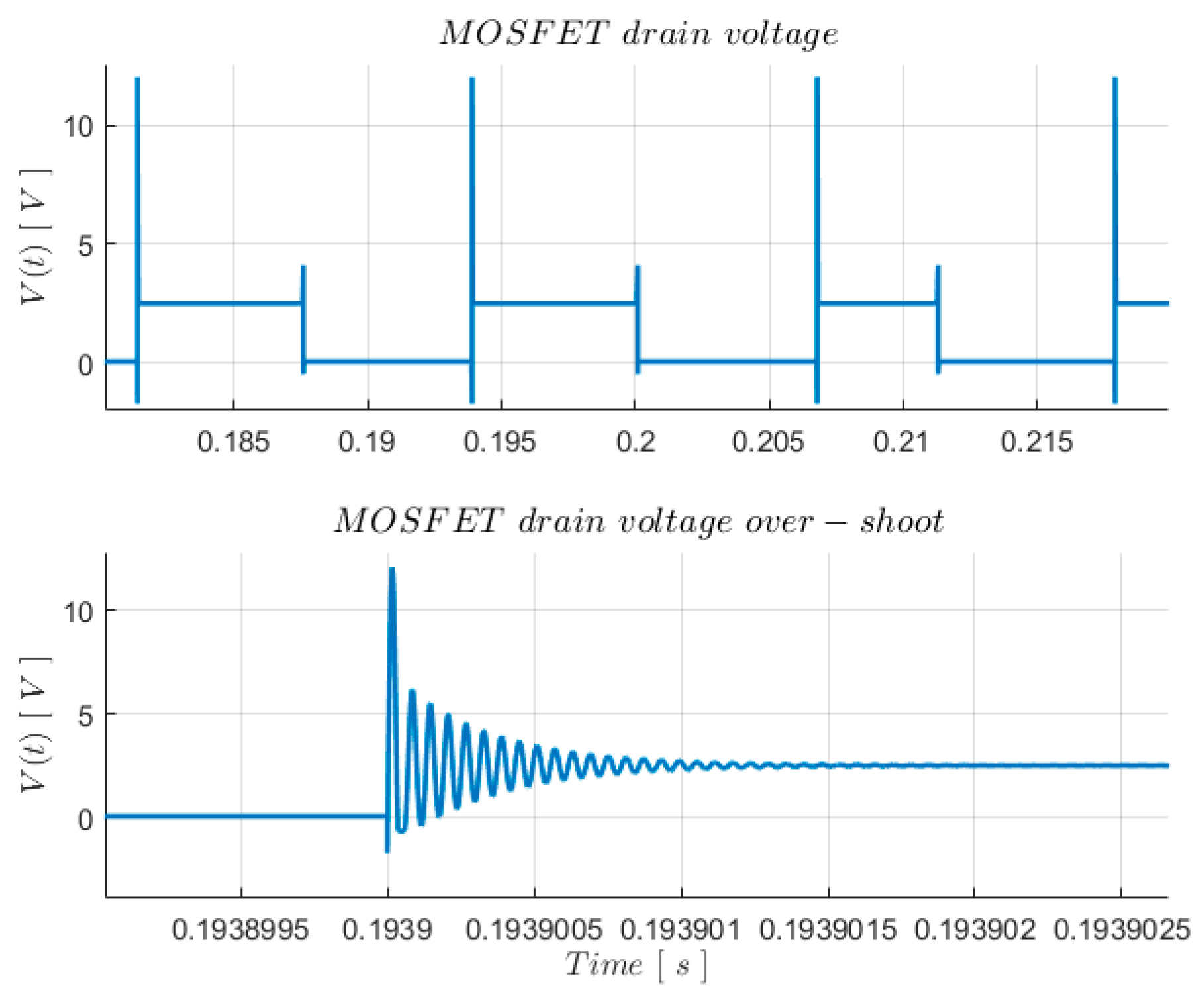
5.5. Results Comparison and Validation
6. Conclusions
Author Contributions
Funding
Data Availability Statement
Conflicts of Interest
References
- Cremona, F.; Lohstroh, M.; Broman, D.; Lee, E.A.; Masin, M.; Tripakis, S. Hybrid co-simulation: It’s about time. Softw. Syst. Model. 2019, 18, 1655–1679. [Google Scholar] [CrossRef]
- Gomes, C.; Thule, C.; Broman, D.; Larsen, P.G.; Vangheluwe, H. Co-Simulation: A Survey. ACM Comput. Surv. 2019, 51, 1–33. [Google Scholar] [CrossRef]
- Jaiswal, S.; Pyrhönen, L.; Mikkola, A. Computationally Efficient Coupling of Multibody Dynamics and Hydraulic Actuators in Simulating Hydraulic Machinery. IEEE/ASME Trans. Mechatron. 2022, 28, 1–12. [Google Scholar] [CrossRef]
- Kaltenbacher, M. Numerical Simulation of Mechatronic Sensors and Actuators: Finite Elements for Computational Multiphysics; Springer: Berlin/Heidelberg, Germany, 2015; ISBN 978-3-642-40169-5. [Google Scholar] [CrossRef]
- Zhao, X.; Liao, X.; Wang, Z.; Wu, G.; Barth, M.; Han, K.; Tiwari, P. Co-Simulation Platform for Modeling and Evaluating Connected and Automated Vehicles and Human Behavior in Mixed Traffic. SAE Int. J. Connect. Autom. Veh. 2022, 5, 313–326. [Google Scholar] [CrossRef]
- Wang, W.; Yang, W.; Dinavahi, V. Co-Simulation Interfacing Capabilities in Device-Level Power Electronic Circuit Simulation Tools: An Overview. Int. J. Power Electron. Drive Syst. 2015, 6, 665–682. [Google Scholar] [CrossRef]
- Reato, F.M.; Cinquemani, S.; Ricci, C.; Misfatto, J.; Calzaferri, M. A Multi-Domain Model for Variable Gap Iron-Cored Wireless Power Transmission System. Appl. Sci. 2023, 13, 1820. [Google Scholar] [CrossRef]
- Wilson, C.G.; Hung, J.Y. A system simulation technique combining SPICE and SIMULINK tools. In Proceedings of the IECON 2010—36th Annual Conference on IEEE Industrial Electronics Society, Glendale, AZ, USA, 7–10 November 2010; pp. 41–46. [Google Scholar] [CrossRef]
- Faruque, M.O.; Dinavahi, V.; Steurer, M.; Monti, A.; Strunz, K.; Martinez, J.A.; Chang, G.W.; Jatskevich, J.; Iravani, R.; Davoudi, A. Interfacing Issues in Multi-Domain Simulation Tools. IEEE Trans. Power Deliv. 2012, 27, 439–448. [Google Scholar] [CrossRef]
- Madbouly, M.; Dessouky, M.; Zakaria, M.; Latif, R.A.; Farid, A. MATLAB—SPICE interface (MATSPICE) and its applications. In Proceedings of the 12th IEEE International Conference on Fuzzy Systems (Cat. No.03CH37442), Cairo, Egypt, 1 December 2003; pp. 37–40. [Google Scholar] [CrossRef]
- Salvaire, F. PySpice. Available online: https://pyspice.fabrice-salvaire.fr (accessed on 5 December 2022).
- Tursini, M.; Villani, M.; Di Tullio, A.; Fabri, G.; Collazzo, F.P. Off-line co-simulation of multiphase PM motor-drives. In Proceedings of the 2016 XXII International Conference on Electrical Machines (ICEM), Lausanne, Switzerland, 4–7 September 2016; pp. 1138–1144. [Google Scholar] [CrossRef]
- Boff, B.H.B.; Flores, J.V.; Flores Filho, A.F.; Eckert, P.R. Dynamic Modeling of Linear Permanent Magnet Synchronous Motors: Determination of Parameters and Numerical Co-Simulation. J. Control Autom. Electr. Syst. 2021, 32, 1782–1794. [Google Scholar] [CrossRef]
- Elleaume, P.; Chubar, O.; Chavanne, J. Computing 3D magnetic fields from insertion devices. In Proceedings of the 1997 Particle Accelerator Conference (Cat. No.97CH36167), Vancouver, BC, Canada, 16 May 1997; Volume 3, pp. 3509–3511. [Google Scholar] [CrossRef]
- Lee, C.-Y.; Chen, Z.-H.; Chang, H.-T.; Wen, C.-Y.; Cheng, C.-H. Design and fabrication of novel micro electromagnetic actuator. Microsyst. Technol. 2009, 15, 1171–1177. [Google Scholar] [CrossRef]
- Shen, Z.; Kaymak, M.; Wang, H.; Hu, J.; Jin, L.; Blaabjerg, F.; De Doncker, R.W. The Faraday Shields Loss of Transformers. IEEE Trans. Power Electron. 2020, 35, 12194–12206. [Google Scholar] [CrossRef]
- Mei, S.; Ismail, Y.I. Modeling skin and proximity effects with reduced realizable RL circuits. IEEE Trans. Very Large Scale Integr. VLSI Syst. 2004, 12, 437–447. [Google Scholar] [CrossRef]
- Costa, E.M.M. Parasitic Capacitances on Planar Coil. J. Electromagn. Waves Appl. 2009, 23, 2339–2350. [Google Scholar] [CrossRef]
- Mohan, S.S.; del Mar Hershenson, M.; Boyd, S.P.; Lee, T.H. Simple accurate expressions for planar spiral inductances. IEEE J. Solid-State Circuits 1999, 34, 1419–1424. [Google Scholar] [CrossRef]
- Bao, M. Circular Diaphragm—An Overview|ScienceDirect Topics. Available online: https://www.sciencedirect.com/topics/engineering/circular-diaphragm (accessed on 6 December 2022).


| Parameter | Value | Unit |
|---|---|---|
| AC resistance: | 2 | |
| Stray capacitance: | ||
| Stray inductance: |
| Parameter | Value | Unit |
|---|---|---|
| Diaphragm radius: | 1000 | |
| Diaphragm thickness: | 100 | |
| Diaphragm surface: | 3.15 | |
| PDMS Young’s modulus: | 550 | |
| PDMS Poisson’s ratio: | 0.5 | |
| Coil current: | 0.6 | |
| Number of turns: | 10 | |
| Magnetic flux density: | 0.0416 | |
| Max deflection @ : | 150 | |
| Equivalent coil length: | 7384 | |
| Equivalent spring stiffness: | 0.0078 |
Disclaimer/Publisher’s Note: The statements, opinions and data contained in all publications are solely those of the individual author(s) and contributor(s) and not of MDPI and/or the editor(s). MDPI and/or the editor(s) disclaim responsibility for any injury to people or property resulting from any ideas, methods, instructions or products referred to in the content. |
© 2023 by the authors. Licensee MDPI, Basel, Switzerland. This article is an open access article distributed under the terms and conditions of the Creative Commons Attribution (CC BY) license (https://creativecommons.org/licenses/by/4.0/).
Share and Cite
Reato, F.M.; Ricci, C.; Misfatto, J.; Calzaferri, M.; Cinquemani, S. An Alternative Multi-Physics-Based Methodology for Strongly Coupled Electro-Magneto-Mechanical Problems. Algorithms 2023, 16, 306. https://doi.org/10.3390/a16060306
Reato FM, Ricci C, Misfatto J, Calzaferri M, Cinquemani S. An Alternative Multi-Physics-Based Methodology for Strongly Coupled Electro-Magneto-Mechanical Problems. Algorithms. 2023; 16(6):306. https://doi.org/10.3390/a16060306
Chicago/Turabian StyleReato, Federico Maria, Claudio Ricci, Jan Misfatto, Matteo Calzaferri, and Simone Cinquemani. 2023. "An Alternative Multi-Physics-Based Methodology for Strongly Coupled Electro-Magneto-Mechanical Problems" Algorithms 16, no. 6: 306. https://doi.org/10.3390/a16060306
APA StyleReato, F. M., Ricci, C., Misfatto, J., Calzaferri, M., & Cinquemani, S. (2023). An Alternative Multi-Physics-Based Methodology for Strongly Coupled Electro-Magneto-Mechanical Problems. Algorithms, 16(6), 306. https://doi.org/10.3390/a16060306