Signal Processing in Optical Frequency Domain Reflectometry Systems Based on Self-Sweeping Fiber Laser with Continuous-Wave Intensity Dynamics

Abstract

We report on the development of an optical frequency domain reflectometry (OFDR) system based on a continuous-wave Er-doped self-sweeping fiber laser. In this work, we investigate the influence of the input data processing procedure in an OFDR system on the resulting reflectograms and noise level. In particular, several types of signal averaging (in time and frequency domain) and Fourier analysis are applied. We demonstrate that the averaging in the frequency domain can be applied to evaluate absolute values of the local scattering amplitudes related to the Rayleigh light scattering (RLS), which is associated with the interference of scattering signals on microscopic inhomogeneities in optical fibers. We found that the RLS signal remains unchanged in the case of signal averaging in time domain, while the noise floor level decreases by 30 dB with an increasing number of points from 1 to ~450. At the same time, it becomes possible to detect the spectral composition of the scattering at each point of the fiber using windowed Fourier transform. As a result, the sensitivity of the developed system allows us to measure the RLS signal at a level of about 20 dB above the noise floor. The described analysis methods can be useful in the development of distributed sensors based on Rayleigh OFDR systems.

1. Introduction

Optical reflectometry (OR) in optical fibers is one of the main techniques for distributed sensing/measurements [1]. Approaches based on OR cover a wide range of temperature, strain, and vibration measurement tasks. The lengths of sensing fibers in such tasks can exceed 100 km [2], while the spatial resolution can reach the sub-millimeter scale [3]. OR is based on the measurements of the local light scattering that occurs as the probe radiation propagates along the fiber. One of the main types of OR is based on Rayleigh light scattering (RLS) [4,5]. It is elastic light scattering at microscopic inhomogeneities of refractive index presenting in cores of all commonly used optical fibers. This htype of OR can be divided into two main branches depending on properties of probe radiation. Pulsed probe radiation with fixed optical frequency and continuous-wave (CW) tunable probe radiation are used in the time and frequency domain in branches of OR, respectively.

Optical time domain reflectometry (OTDR) is based on measurements of scattered/reflected signals produced through short (nanosecond) pulses. As a pulse propagates along the fiber, the scattered/reflected signal returns back to the laser source with a time delay proportional to the distance between the laser and the local scatterer/reflector [6]. The result of OTDR is a reflectogram demonstrating a dependence of the reflection amplitude/scatterer density on the fiber longitudinal co-ordinate. In this case, the maximum sensing line length is limited only by the fiber losses and reaches tens of kilometers [7]. At the same time, the spatial resolution is limited by the pulse duration and is typically in the order of units of meters [7].

In turn, in the case of optical frequency domain reflectometry (OFDR), the local response can be also connected with scattered signal delay. However, analyzed signals are measured in interferometric two-beam configuration, in which coherent probe radiation with optical frequency tuning is used to construct an interferogram. Relative delay between scattered and reference signals passed through the test and reference arms of the interferometer, respectively, is contained in frequency of spectral oscillations of the interferogram [8,9]. Spectral analysis of such interferogram with Fast Fourier transform (FFT) makes it possible to construct a reflectogram and achieve high spatial resolution (units or even fractions of mm) at the expense of the sensing fiber line reduction [10]. The sensing lines usually have lengths of several tens of meters. Such sensing lines are useful for distributed testing various systems and components, the detection of cracks, and construction health monitoring [11,12].

OFDR requires use of highly coherent laser sources with frequency tuning capability. The use of Fourier analysis imposes strict requirements on the linearity of frequency tuning. As a rule, semiconductor tunable lasers are used as sources of probe radiation sources. Such lasers typically have non-linearity in the optical frequency tuning rate [10]. In the vast majority of OFDR articles and patents, this problem is solved either via using additional methods to linearize the laser frequency tuning [13,14] or measuring the laser frequency and further compensating the non-linearity [15,16,17]. An alternative to this approach is the use of lasers with frequency changing in stepwise manner with fixed frequency steps. In case of stepwise frequency tuning, the linearity is achieved a priori without the need for correction via external means. One implementation of such a source is a fiber self-sweeping laser [18]. An important feature of such lasers is that the optical frequency tuning occurs due to internal processes related to the formation of dynamic filters based on population inversion gratings [18], which are found directly in the active medium during laser generation, without the need for any additional external filters. In such lasers, the optical frequency changes in stepwise manner from pulse to pulse using a fixed value (~2–20 MHz) determined based on the laser cavity length.

The first OFDR systems based on a self-sweeping fiber laser (see [19] and references therein) previously showed satisfactory characteristics. The OFDR system had spatial sampling of ~200 µm, sensitivity of about −79 dB (or −86 dB/mm), and a test line length of up to ~9 m. The sensing tasks related to measuring a spatial distribution of physical quantities with OFDR systems are of general interest for various practical applications. However, due to insufficient sensitivity of first OFDR systems based on self-sweeping lasers, the first results were far from realization of distributed measurements in lines under test (LUTs) based on conventional passive fibers. In order to increase levels of measured signals, a LUT consisting of an array of non-resonant was used. The FBGs reflection maxima did not match the tuning range of the probe laser. However, the sensitivity of the reflectometer was sufficient enough to register the probe radiation scattered via the non-resonant FBGs and demonstrate the possibility of quasi-distribute temperature measurements. In particular, it was shown that the correlation analysis makes it possible to determine the temperature of each FBG in the array. An additional optimization of the OFDR system interferometer was important to increase the visibility of the interference spectra for measuring weak scattered signals [19]. It was shown that the optimization can improve the system sensitivity down to −110 dB/mm. As a result, the possibility of truly distributed temperature measurements with an OFDR system based on RLS with the self-sweeping laser radiation was also demonstrated.

Moreover, the signal processing techniques are of great importance for the development of OFDR systems designed to measure weak signals, such as RLS. Different noise sources introduced through the laser instabilities, measurement system components, and the environment fluctuations can make it difficult to extract information about the magnitude of the scattering amplitude in LUTs. When an OFDR system is used to measure changes in temperature or strain along a sensing line, additional analysis of measured reflectograms is required. Thus, the development of approaches for OFDR signals processing is of great interest.

In the present work, we investigate the influence of the input data processing procedure in an OFDR system based on a self-sweeping laser on the resulting reflectograms and noise level. An Er-doped self-sweeping laser with continuous-wave (CW) intensity dynamics [20] was used as a probe radiation source. The main feature of the probe source was the generation of relatively long (~ms) and highly coherent mode pulses. Long pulse duration enables improvement of the processing algorithms because there is a possibility of long accumulation of measured signals. It should be noted that such a possibility was not considered in previous OFDR systems based on pulse self-sweeping lasers (for example, [19]) because of the much shorter single-frequency generation time. It is found that averaging in the time domain leads to a significant decrease in the noise floor level (NFL). In particular, an increase in the number of averaging points from 1 to 430 decreases the NFL by 30 dB. For low numbers of averaging points (1–2), the level of RLS appears to be lower than the NFL; thus, long signal accumulation significantly improves the system performance. Finally, averaging in the frequency domain can be carried out via scanning the central frequency; however, this approach leads to a loss of information on the spectral composition of the RLS signal. The described analysis methods can be useful in the development of distributed sensors based on Rayleigh OFDR systems.

2. Theoretical Part

An optical scheme of a typical OFDR system is shown in Figure 1. Radiation from a tunable laser source entered a Mach–Zehnder interferometer (MZI) formed of two couplers: a circulator and a LUT. The tunable probe laser radiation was split at coupler 1 between the reference and probe arms of the MZI. In the former arm, radiation was directed to coupler 2, while in the latter arm, it passed through the circulator. After passing through the circulator, the probe radiation entered the LUT, and the scattered/reflected signal passed through the circulator again and interfered with the other signal from the reference arm at the coupler 2. In the case of distributed measurements, the LUT was represented as a set of many local reflectors. We noted, however, that every particular position of a reflector corresponded to a fixed difference between the lengths of the reference and probe arms of the interferometer ΔL. The interference signal measured at output of the MZI E_out(ν) is given via the following expression:

$$E_{out}=E_1^2+E_2^2+2\sqrt{E_1{E}_2}·sin\left(\frac{2\pi v\mathsf{\Delta }L}{c}\right),$$

(1)

where E₁, E₂ are the amplitudes of the probe and reference radiation electric fields at output of coupler 2, c is the speed of light, and v is the probe laser optical frequency. In the case of the point reflector, the output signal has the sine function dependence on the laser frequency v. If many local reflectors are present and distributed along the LUT, the output signal becomes a superposition of such sine functions with different amplitudes and periods. An example of a local reflector placed at three different positions in the LUT is demonstrated in Figure 1, together with corresponding sinusoidal transmission functions shown in red, green, and blue for near, middle, and far positions, respectively. The FFT was applied to the spectral transmission function to find the MZI arms difference (time delay) associated with each reflector. In this case, the amplitude of each sine function corresponding to the reflection amplitude for each local reflector was reconstructed. In the case of OR based on RLS, the scattering centers acted as such local reflectors.

Here we describe the situation that occurred when a continuous-wave self-sweeping laser [20] was used as a tunable radiation source. The tuning process occurred in a stepwise manner (Figure 2a). In this case, the consecutive horizontal sections with duration T were divided by a fixed value in the frequency domain—frequency tuning step δν—which was determined through the parameters of the laser cavity. In this case, optical frequency within each horizontal section could be considered constant (its fluctuation within each section did not exceed 50 kHz [20]). The duration of each section was equal to the duration of the mode pulse T and was of the order of several ms. Confirmation of these results was presented in [20], where a detailed analysis of the laser mode dynamics was carried out. When the radiation with stepwise change in the optical frequency passed through the MZI, an amplitude modulation appeared at the output with stepwise modulation in the transmitted power (Figure 2b). The signal from the MZI output was then digitized. The number of points per unit of time in the resulting signal was the signal sampling rate. As a result, sets of amplitudes of the incident transmitted through the MZI waves were recorded for each optical frequency.

To calculate the reflectograms (Figure 2c), FFT was applied to the MZI output signals plotted as a function of the pulse number. It is known that the maximum length of LUT L_max corresponding to the highest frequency modulation is limited through the frequency tuning step δν in the following way:

$$L_{max}=\frac{c}{4n\delta \nu },$$

(2)

where n is the refractive index in the LUT. In turn, spatial sampling δl in the reflectogram was limited to the maximum probe laser tuning range Δν, i.e., by the product of frequency tuning step and the number of mode pulses used in the reflectogram calculation, as follows [21]:

$$\delta l=\frac{c}{2n\mathsf{\Delta }\nu }.$$

(3)

A key feature of the self-sweeping laser used in the study was the strict discreteness of the optical frequencies of the sequentially generated mode pulses, which was defined through the fixed length of the laser cavity. For such a source, the dependence of the optical frequency on the pulse number was a linear function. For this reason, the problem of tuning non-linearity compensation observed in the time domain and described in the introduction was solved automatically during the transition from time to mode pulse numbers.

It should be mentioned that the window function could be properly selected for processing measured signals with the FFT in OFDR systems, especially when a strong reflector presents in a LUT. We illustrate this issue with a numeric example. According to Expression (1), the model signal was the sine sampled at discrete coordinates (black line in Figure 3a). To evaluate a reflectogram corresponding to this signal, we performed the FFT with a rectangular window (black solid line in Figure 3b). The reflectogram had a single peak with an amplitude of 0 dB centered at the modulation frequency. It had wide wings corresponding to the instrument. The wings were located at a relatively high level of ~ −35 dB. However, it was known from [22] that the sinusoid length had to be properly selected to meet the condition of periodicity over the considered sampling interval and reduce the wings’ amplitudes in this way. Thus, the number of sampling points was reduced to be closer to a multiple of the sine period (see the red line in Figure 3a), and a sharp decrease in the instrument function wings level down to −70 dB (red solid line in Figure 3b) was observed. This behavior related to the spectral leakage effect [22]. Another approach to reduce the level of the instrument function wings was to change the shape of the FFT window function. The Hann window is one of the most commonly used window functions [22,23]. When the Hann window was used, the level of the instrument function wings decreased down to −100 dB at a large distance from the central peak (black dashed line in Figure 3b). However, a significant broadening of the central peak occurred in this case. It was noted that despite the use of a different window, the proper selection of the sinusoid length worked similarly in this case. The red dashed line in Figure 3b corresponded to the FFT with the Hann window in the case where the number of points became closer to the multiple of the sine function period. However, in this case, the wings level did not decrease as significantly as in the previous case. Moreover, the instrument function stayed wider compared to the FFT rectangular window function. Thus, when selecting the window function, it was necessary to maintain balance between the width of the central peak and the level of the instrument function wings. When processing the experimental signals, we further used FFT with Hann window function.

3. Experimental Setup

Initially, we describe the probe radiation source used during the experiment. An Er-doped CW self-sweeping laser with ring cavity was used as the radiation source. The dynamics of an identical laser were described in detail in [20]. The laser provided wavelength tuning in the 40–50 pm (5–6 GHz) range near the wavelength of 1565 nm. The laser radiation was a sequence of long weakly overlapping pulses with a rectangular intensity profile corresponding to the successive generation of neighboring longitudinal modes. Figure 4a,b shows the evolution of the optical frequency of the laser and the intensity dynamics of sequentially generated longitudinal modes, respectively [20]. Different colors in Figure 4b corresponded to different laser cavity modes. As a result, the laser integral (over simultaneously generating modes) intensity dynamics, which was measured at the output of the laser and presented in Figure 4c, is a CW signal with short intensity bursts occurring with a period of T~1 ms. The bursts corresponded to the rapid change in mode composition with simultaneous generation of two neighboring modes, when there is a rapid (~100 µs) increase in one mode and a fading in the other. The frequency tuning step between two neighboring modes was δν = 9.7 MHz. During a single mode pulse, the radiation is highly coherent with linewidth not exceeding 40 kHz [20]. Thus, this laser used in OFDR systems provided a maximum sensing line length of L_max~5.35 m and spatial resolution of δl~2 cm, according to Expressions (2) and (3), respectively. Considering the preliminary data processing analysis of the interferograms, it was essential to conclude that the laser generation consisted of a sequence of long (T~1 ms) sections with fixed optical frequency separated by short transitions with a fixed value of optical frequency change (δν = 9.7 MHz).

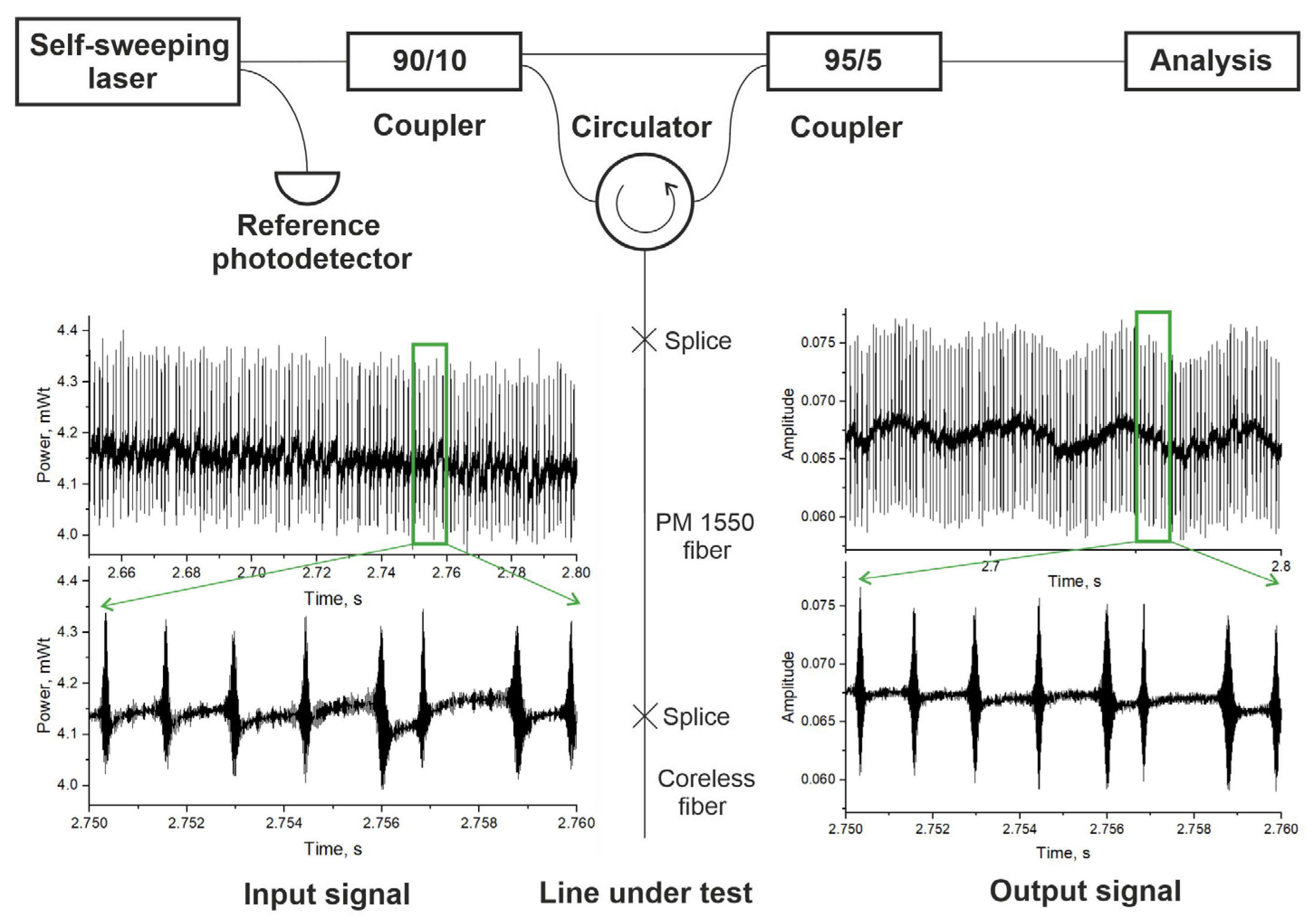
The scheme of the experimental OFDR system is shown in Figure 5. The OFDR system was based on polarization-maintaining (PM) fibers and components. The radiation of the probe self-sweeping Er-doped fiber laser described above was divided into two parts using an additional fiber coupler. The first part was used as a reference signal for normalization in order to eliminate the influence of the laser output power fluctuations. The other part entered the MZI formed using the input and output couplers with coupling coefficients of 10% and 5%, respectively, and a circulator connected to a LUT. In our experiments, a piece of 1.6 m long PM fiber with short (0.2 m long) coreless fiber spliced at the far end was used as the LUT. The coreless fiber minimized the influence of the Fresnel back reflection coming from the far end of the LUT, since the radiation propagating inside the coreless fiber diffracted rapidly (experiencing huge losses) and did not actually reach the end of the LUT. The signal scattered/reflected in the LUT returned back to the circulator and was redirected to the output coupler, where it interfered with the other portion of radiation coming from the reference arm of the MZI. The laser power after passing the MZI reduced to a few tens of microwatts. It was noted that the MZI was vibro-isolated from the environment fluctuations using foam rubber. A digital oscilloscope (LeCroy Wavesurfer 3034R, USA) was used for data recording. A fast photodetector (PD) Thorlabs DET08CFC was used to measure the reference signal at the output of the probe laser (input of the MZI). The interference signal was measured at the MZI output with an InGaAs switchable gain amplified PD (Thorlabs PDA20CS2, USA) used in 10 dB gain mode. The typical signals measured at the input and output of the MZI are shown in the left and right insets of Figure 5, respectively. We can see from the insets that additional amplitude modulation appears at the MZI output, which contains information about positions and amplitudes of reflectors/scatters in the LUT. Thus, the main task of the signal processing procedure was an accurate extraction of the interferogram from the measured signals with the highest possible signal-to-noise ratio (SNR). Analyzing zoomed views of the signals shown in the bottom of Figure 5, we noted that the signal levels observed during generation of individual mode pulses are not quite constant. The observed slight signal increase was related to the PDs inertia. In spite of the large bandwidth (MHz level) of the PDs suitable for measuring sub-microsecond signals, we observed slow residual growth of the signals’ amplitudes at millisecond time scale. To reduce the influence of this slow growth of the measured signals levels on the interferogram extraction result, we used an additional variable resistor to increase load impedance for the reference PD and make this growth identical for both PDs. In our case, this approach corresponded to the reference PD load impedance of about 2 kOhm. As a result, the bandwidths of the reference and signal PDs were estimated to be 25 and 1.5 MHz, respectively.

4. Data Processing

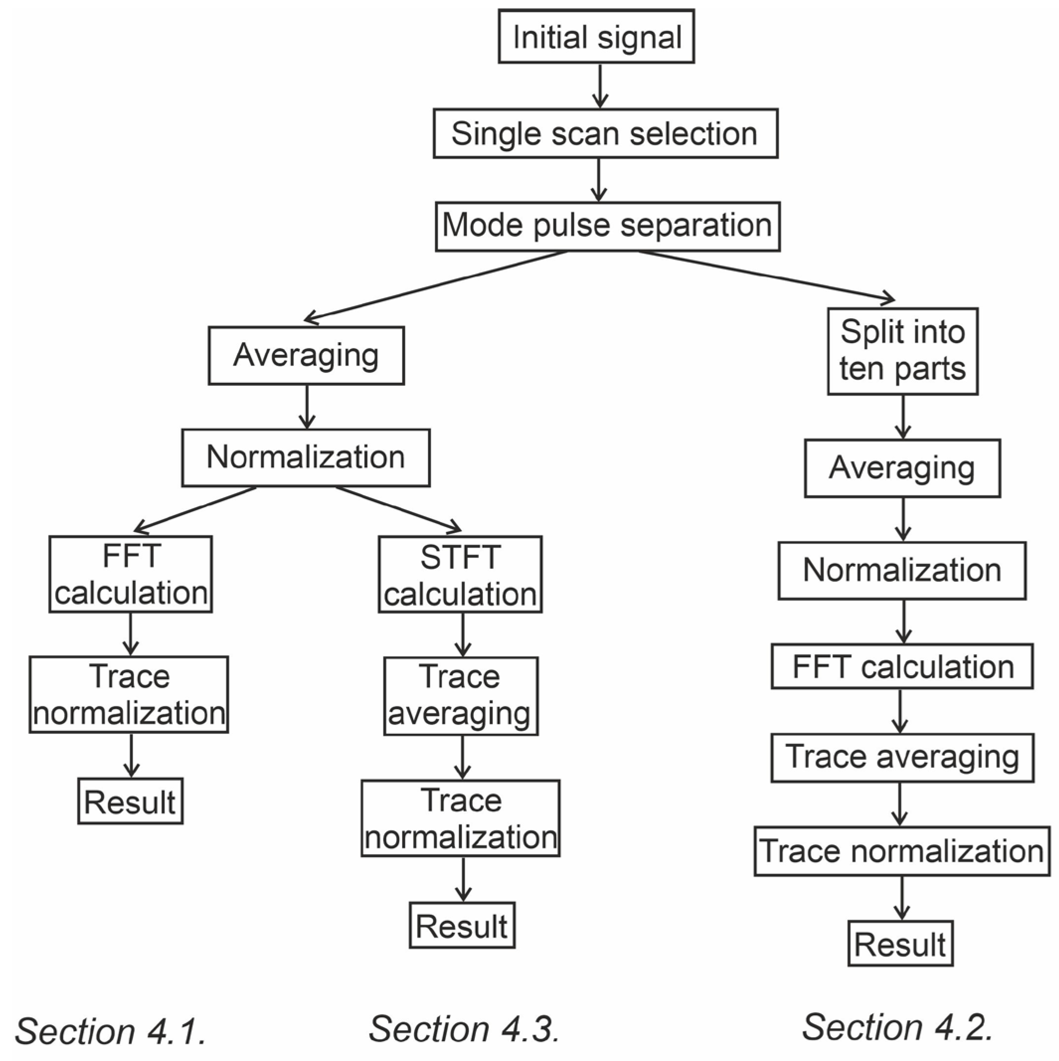
As described above, the main task of the signal processing procedure is the accurate extraction of the interferogram with the highest SNR. The signal processing consisted of several steps: (1) splitting the signal into individual sweeping scans; (2) splitting the signal into individual mode pulses; (3) normalizing the interference signal (I) measured at the MZI output in relation to the corresponding reference one (R) measured at the input; and (4) calculating the FFT. The averaging can be carried out after each of these steps depending on the task of the LUT characterization. We now consider different averaging approaches and their effects on the final result.

As described above, the main task of the signal processing procedure is the accurate extraction of the interferogram with the highest SNR. The signal processing consisted of several steps: (1) “Single scan selection”, which involved splitting the signal into individual sweeping scans; (2) “Mode pulse separation”, which involved splitting the signal into individual mode pulses; (3) “Normalization”, which involved normalizing the interference signal (I) measured at the MZI output in relation to the corresponding reference one (R) measured at the input; and (4) “FFT calculation”, which involved calculating fast Fourier transform (FFT) or short-time Fourier transform (STFT). The averaging can be carried out after each of these steps depending on the task of the LUT characterization. We then consider different averaging approaches and their effects on the final result. Different analysis algorithms are summarized for convenience in the way of a flow diagram, as shown in Figure 6.

The first step in the processing algorithm was the selection of the signal interval corresponding to only one frequency scan for further analysis. The scan selection technique was based on the fact that the average laser output power slightly decreases from the beginning to the end of each scan. In the case of the laser used in our study, a single scan consists of 300–500 single-frequency mode pulses, which are separated using a frequency tuning step of δν = 9.7 MHz in frequency domain. It is important to note that the pulse duration fluctuations do not affect the value of the frequency tuning step. All further signal processing is performed for only one scan. In this case, the optical frequency depends linearly on the pulse number a priori, since all the frequency hops during a single scan have the same direction and equal values. A confirmation of this fact was demonstrated in a previously published paper [20], where a detailed study of the mode dynamics of this particular Er-doped self-sweeping laser was carried out using optical homo- and hetero-dyning analysis.

At the second step, the separation of the MZI output and reference signals into sections corresponding to different mode pulses is performed. For this purpose, all intensity bursts are found. Furthermore, all points associated with transitions between mode pulses (areas highlighted in red in Figure 7) are removed from consideration. The reference signal is used to find the bursts because the average level of the reference signal remains practically unchanged during the frequency tuning (in contrast to the MZI output one), simplifying detection of the intensity bursts. As a result of this separation, we construct two vectors of pulse amplitudes (R_i,j and I_i,j) for length J for every i-th pulse that has fixed optical frequency. Here, index j denotes the number of the j-th element in the i-th vector. The pulse length J varies from pulse to pulse due to small (~20%) fluctuations in their duration.

In the most straightforward signal processing algorithm, averaging over the entire length of the array corresponding to a single-mode pulse is performed:

$$\begin{gathered} I_i={〈I_{i.j}〉}_{j=0..J}=\frac{1}{J}{\sum }_{j=1}^J{I}_{i.j}, \\ {R}_i={〈R_{i.j}〉}_{j=0..J}=\frac{1}{J}{\sum }_{j=1}^J{R}_{i.j}. \end{gathered}$$

(4)

Hereinafter, the time domain averaging will be denoted using angle brackets. The number of averaging points J for a given pulse depends both on the oscilloscope sampling rate and the data processing algorithm. The results of the averaging for the first pulse (numbered as i − 1) are presented in Figure 7a,b using green circles for the reference and MZI output signals.

4.1. Time Domain Averaging before Normalization

Here, we describe the processing procedure and the reflectogram calculation when all points of the mode pulse are used for averaging (green circles for the (i − 1)-th pulse in Figure 7a,b). The pulse-by-pulse normalization procedure is then performed: $S_i=\frac{I_i}{R_i}$. As mentioned above, correct pulse-by-pulse division is possible only when the growth rates of the signals in both channels are equal. Finally, the FFT from the final signal is calculated: $F=\widehat{F}\left(S_i\right)$. The optical frequency coordinate (optical detuning) is transformed to the longitudinal coordinate according to the following expression:

$$z_k=\frac{c·k}{2·N·\delta \nu },$$

(5)

where k is the and N are the FFT vector index and length, respectively, and c is the speed of light. For correct comparison, different reflectograms were additionally normalized to the level of 0 dB at zero FFT frequency (in other words, the signal levels were normalized to the average transmitted power). It should be noted that absolute values of reflection amplitudes depend on the coupling ratios of couplers used for the MZI [19]. Thus, additional system calibration is required for the absolute values measurements.

The resulting reflectograms are presented in Figure 8a. In this figure, we tried to trace a dependence of the reflectogram calculation results on the number of averaging points. Thus, we used original data with the maximum sampling rate (green curve in Figure 8a) and reduced the number of points used in calculations. For example, only the first 10 points after the bursts are used for the calculation of blue line in Figure 8a. It should be noted that the legend of Figure 8 indicates, in fact, the number of averaging points J measured at a fixed optical frequency ω_i averaged over different pulses. The number of averaging points J fluctuates with pulse-to-pulse fluctuations of the mode pulses duration. We note that although the average number of points changes by two orders of magnitude, the characteristic features remain in different reflectograms. For example, a sharp decrease in reflectograms is present in all the graphs (except for black and red ones) at the coordinate z~2.2 m, which corresponds to the end of the LUT. We can conclude that a higher signal level observed at shorter lengths (z < 2.2 m) corresponds to RLS, while a lower signal level (at z > 2.2 m) corresponds to the NFL. Next, a peak with an amplitude of −40 dB is observed at the coordinate z = 0.4 m, which corresponds to the location of a circulator used in the MZI. The peak corresponds to scattered radiation inside the circulator directly from port 1 to port 3. Moreover, a couple of peaks with much smaller amplitudes are noticed in the noise signal at the coordinates z = 4.4 and z = 4.8 m. However, the positions and amplitudes of these peaks did not depend on the LUT configuration. Thus, we conclude that these peaks are associated with parasitic modulation in the electrical part of the scheme.

We also note that the appearance of the reflectogram near the noise floor does not remain constant. The useful signal on the reflectograms, which corresponds to the RLS, has the same structure (alternating dips and peaks). However, the NFL and dips and peaks in the noise floor change their positions and amplitudes as the number of averaging points increases (see black squares in Figure 8b). The increase in the number of averaging points from 1 to 430 points results in a significant decrease in NFL of ~30 dB (Figure 8b). The red line in Figure 8b corresponds to the RLS level.

4.2. Time Domain Averaging after Normalization

Since these results show weak dependence on the number of averaging points, the analysis procedure is modified. After dividing the signals into sections corresponding to separate mode pulses, we also separate each section into several intervals. Figure 7 shows the separation of the i-th mode pulse into 10 equal intervals with green vertical lines. Thus, the mode pulse consisting of J points is divided into 10 intervals, within which preliminary averaging was performed. As a result, each of the mode-pulses was connected with two sets of ten average values. If we make J a multiple of 10 through eliminating excessive points, the averaging procedure is performed as follows:

$$\begin{gathered} I_i^{\left(1\right)}={〈I_{i.j}〉}_{j=0,\dots ,\frac{J}{10}} \\ \dots \\ {I}_i^{\left(n\right)}={〈I_{i.j}〉}_{j=\frac{J\left(n-1\right)}{10},\dots ,\frac{Jn}{10}} \\ \dots \\ {I}_i^{\left(10\right)}={〈I_{i.j}〉}_{j=\left(J-\frac{J}{10}\right),\dots ,J}. \end{gathered}$$

(6)

The blue circles in Figure 7a,b show the average values for the second interval of the i-th mode pulse ($I_i^{\left(2\right)}$ and $R_i^{\left(2\right)}$, respectively). Next, 10 data arrays corresponding to different intervals of the mode pulses are constructed for the reference and MZI output signals, and the corresponding normalization of the signals are made:

$$S_i^{\left(n\right)}=I_i^{\left(n\right)}/R_i^{\left(n\right)}.$$

(7)

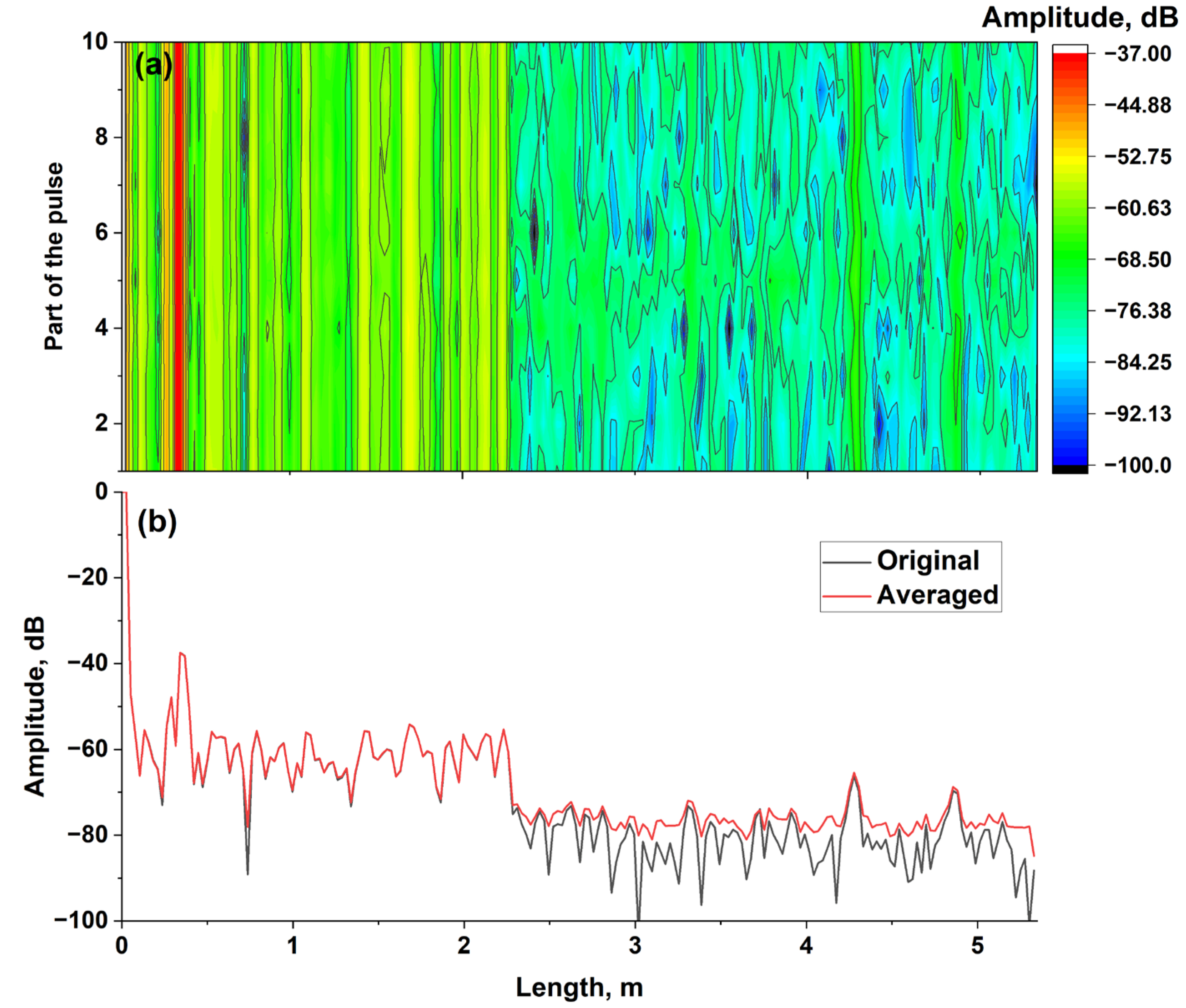
Therefore, the normalization is performed in this case for individual parts of the mode pulses, and we produce 10 interferograms on the basis of these S_i⁽ⁿ⁾ values, taking every n-th section from each of the pulse. Individual reflectograms corresponding to the interferograms are calculated through taking the FFT: $F^n=\widehat{F}\left(S_i^{\left(n\right)}\right)$. The calculation result is presented as a heat map in Figure 9a. The horizontal and vertical axes correspond to the coordinate along the LUT (z) and the number of the interval used for the reflectogram construction, respectively, while color corresponds to the amplitude. It can be noted that while the part of the reflectogram corresponding to the noise floor changes quite chaotically with variation in the mode pulse section, the other part at z < 2.2 m (corresponding to the RLS) only slightly changes. There are vertical bands in the RLS parts of the reflectograms, indicating that, for a fixed LUT coordinate, the signal remains constant, regardless of the number of a particular interval used for the calculations.

Since the signal corresponding to the LUT does not change, it is possible to average the reflectograms corresponding to different sections of the mode pulses (i.e., using the number n). The result is represented via the red curve in Figure 9b. For comparison, the signal obtained after the averaging over the entire mode pulse is also shown. It can be seen that the signal for z < 2.2 m is the same for signals shown in Figure 8a and Figure 9b. In turn, the NFL increases, while fluctuations of the noise signal decrease.

4.3. Frequency Domain Averaging

In all approaches described in the above text, the reflectograms are obtained using the data from a fixed-frequency tuning range Δν of the probe laser. We conclude that the structure of the signal corresponding to the LUT remains constant and does not depend on the nature of averaging. Moreover, we consider thr influence of the laser tuning range position (the central optical frequency position within a scan) on the reflectogram at a fixed length of the spectral range (window length). In this case, we consider a longer scan and move the position of the data range used for processing. For this purpose, the data were first averaged over each mode pulse and pulse-by-pulse normalized, as described above. The windowed (short-time) Fourier transform was then applied to the normalized signal:

$$F_k\left(m\right)=\widehat{F}\left(S_i\right),$$

(8)

where m is the window number. The window length is chosen to be 256 points, corresponding to the tuning range Δν~2.5 GHz with a frequency tuning step between neighboring points of 9.7 MHz. The overlap of the windows was set to 255 points to observe point-by-point variation in the reflectograms. Thus, the sweeping of the central frequency with a fixed value for the frequency tuning range is effectively carried out. The result is shown as a heat map in Figure 10a. The horizontal and vertical axis correspond to the coordinate along the measuring line (z) and the detuning of the central frequency. As before, a sharp decrease in amplitude is present at z = 2.2 m. However, the amplitude of the signal corresponding to the LUT (z < 2.2 m) now depends on the central optical frequency. We conclude that the results of such a line interrogation can be used for sensing tasks, similarly to the distributed temperature measurements performed using a pulsed self-sweeping laser [19]. In addition, the third type of averaging becomes possible: averaging of reflectograms corresponding to different central frequencies (i.e., averaging in the frequency domain). Figure 10b shows a comparison between the original reflectogram (black line) and the result of frequency domain averaging (red line). It can be seen that the fast signal fluctuations now decrease in both regions of reflectogram corresponding to the LUT and the noise floor. It can be expected that with a further variation in the central frequency (vertical axis in the Figure 10a), the reflectogram will become even more smooth, becoming similar to measurement results usually observed in conventional incoherent RLS reflectometry.

5. Discussion

As a result, different algorithms (Figure 6) were applied to calculate reflectograms for the same data set corresponding to one spectral scan. In this case, the measurement time was fixed automatically for all of the calculated reflectograms. Nevertheless, we tried to model the reflectorgams evaluation for measurements with shorter pulses. In particular, we compared reflectograms with different numbers of averaging points, simulating a change in the duration of mode pulses, (4.1) and averaging over a set of traces obtained using different time intervals for the same pulses, (4.2). As a result, it can be concluded that this type of the averaging procedure significantly affected the character of the final trace. The order of normalization and averaging procedures had a strong influence on the NFL. The NFL after averaging 10 reflectograms is ~3 dB higher than after regular time-domain accumulation of the signal (while keeping the total value of data points fixed). This result can be associated with the fact that the normalization procedure was not commutative with averaging and FFT. However, fluctuations in the reflectograms at coordinates corresponding to the noises decreased when averaging over 10 reflectograms corresponding to different of measured signals were used (red line in Figure 8). The useful signal (corresponding to RLS or point reflectors) remains constant in the case of temporal averaging, regardless of the normalization order. This result must be connected to the fact that the reflectograms calculated from different sections of the mode pulse are equivalent due to the preservation of the spectral and phase properties of the self-sweeping laser throughout the generation of each pulse. However, the signal level begins to increase significantly when the number of averaging points decreases to ~1–2 due to the excess in the NFL level over the RLS level. It should be noted that in the OFDR systems based on pulsed self-sweeping lasers [19], the number of points used for the signal accumulation and reflectograms calculation was relatively small (~5) due to the short duration of each pulse. In the present work, a continuous-wave self-sweeping laser with generation of long (~few milliseconds) single-frequency pulses was used. In this case, there is a possibility for long signal accumulation for calculation of a single reflectogram. This outcome eliminates both the need for synchronization of measurements of different scans, which is typical for faster seeping with shorter pulses, and the problem of optical frequency stabilization during slow sweeping, because both the frequency tuning step and generation frequency set are fixed in our case. In addition, the generation of long pulses opens the possibility of signal accumulation for each frequency. It has been shown that time domain averaging makes it possible to significantly (up to ~30 dB) reduce the NFL when the number of points is increased from 1 to ~450 (i.e., by ~27 dB). It can be expected that if the system noises are dominated by the amplitude ones, the NFL should be proportional to a square root of the number of averaging points, i.e., the NFL slope as a function of the number of averaging points should be ~0.5 dB/dB [24]. On the other hand, the reflectograms are calculated as the FFT amplitude (20log instead of the usual 10log), hence the slope should be 1 dB/dB instead of 0.5 dB/dB. Nevertheless, Figure 8b shows non-linear dependence with a higher slope of 2 dB/dB at a small number of averaging points and smaller slope (down to 0.5 dB/dB) for a larger number of averaging points. The slope reduction itself can be interpreted as saturation when the nature of dominant noises becomes different (e.g., the noises related to the bit depth of the signal digitalization). Moreover, the smaller decrease slope for the NFR may be related to the effect of the normalization procedure. This issue requires further research.

It should also be noted that the structure observed in the heat map (Figure 9a) confirms that the longitudinal structure of the RLS signal is not of noise nature. If it was related to noise, the structure of the reflectogram would change for different sections of the pulses used in the processing, which is not the case. This structure contains information about local scattering centers in the LUT. Moreover, the amplitude in the reflectogram at each point of the fiber is not simply the value of the scattering amplitude, but the result of the interference of signals scattered within a small area of size δl determined using the Expression (3). The result of the interference depends on both the fluctuations of the scatterer density within the region δl (fluctuations of the refractive index in the LUT core) and the optical frequency of the radiation. The random nature of the refractive index fluctuations causes an irregular pattern in the part of the reflectogram corresponding to the RLS. This effect is of the same nature as the fading effect observed in C-OTDR systems, where the interference can result in zero integral scattering in some regions of the LUT.

The above-mentioned dependence of the interference result on the optical frequency can be observed in Figure 10a. As the center frequency is tuned, the interference result changes for each LUT segment. Effectively, the scattering spectrum is scanned for each LUT segment. The vertical slice in Figure 10a corresponds to the spectrum at a particular LUT coordinate and contains information about the spectral dependence of the interference of the scattered signals. As a result, the fading effect can be eliminated in the case of the frequency domain averaging. The averaging makes fast oscillations in the reflectograms smoother, but leads to the loss of information about the spectral characteristics of the LUT. In other words, the red line in Figure 10b with averaging reflectograms over the spectrum makes the measurements of the local integral scattering absolute values more accurate at the expense of spectral effects. Thus, averaging in the frequency domain affects not only the NFL, but also the shape of the useful signal.

The choice of averaging approach should be determined based on the task to be solved via the OFDR system under development. For distributed temperature and strain measurements, it is necessary to fix the reference reflection spectrum from the frozen inhomogeneities and study its evolution over time using correlation analysis methods. In this case, only averaging in the time domain or over different sections of the mode pulses can be used to increase the contrast between the useful signal and the noise floor and reduce the fluctuations. In turn, frequency domain averaging can be used to measure the absolute value of the scatter/reflectance, thereby reducing the useful signal fluctuations.

6. Conclusions

In conclusion, the OFDR system based on the probe Er-doped self-sweeping fiber laser is developed. It is demonstrated that the sensitivity of the system allows us to measure the RLS signal at level of about 20 dB above the NFL. The RLS results in the appearance of a complex structure consisting of alternating spatial peaks and dips in measured reflectograms. This structure does not change when the time domain averaging parameters are changed and remains unchanged even when each mode pulse is divided into several independent sections. This structure is associated with the interference of back-scattered signals originating from neighbor sections within a scattering volume, which is limited due to the spatial resolution of the OFDR system. The results of the interference depends on microscopic inhomogeneities in the LUT. In turn, the NFL changes with the number of averaging points: an increase in the number of averaging points from 1 to 430 points decreases the NFL by 30 dB. If the center frequency is tuned using the widowed Fourier transform within the probe laser scanning range, it becomes possible to detect the scattering spectra at each point of the LUT. If some spectral response distribution is recorded via an OFDR system and fixed as a reference, it may become possible to extract information about external impacts on the fiber state caused by heating or deformation. For this purpose, correlation analysis can be applied. This possibility will be investigated in our future research. In addition, averaging in the frequency domain can be performed to specify the information about the absolute value of the local scattering. However, the information about the spectral composition of the scattered signal will be lost in this case. The described analysis techniques can be useful in the development of distributed sensors based on Rayleigh OFDR systems.