
From Activity Recognition to Simulation: The Impact of Granularity on Production Models in Heavy Civil Engineering

 , , and
Abstract
1. Introduction
- RQ1: What impact does production model granularity have on activity recognition?
- RQ2: How does production model granularity affect the application of DTC?
- RQ3: What is needed to adopt production models for DTCs in heavy civil engineering?
2. Related Work
2.1. DTC and Data-Driven DES Modeling
2.2. Activity Recognition Modeling
2.3. Production System Models
2.4. Research Gap and Objective
3. Methodology
- Activity data: While producing the pile, workers manually recorded activities on site with a tool provided by fielddata.io (a German start-up, now acquired by the BAUER Group). They had a choice of 27 predefined activities. The tool was connected via the equipment’s Wi-Fi to have the same time stamps as the sensor data.
- 3.
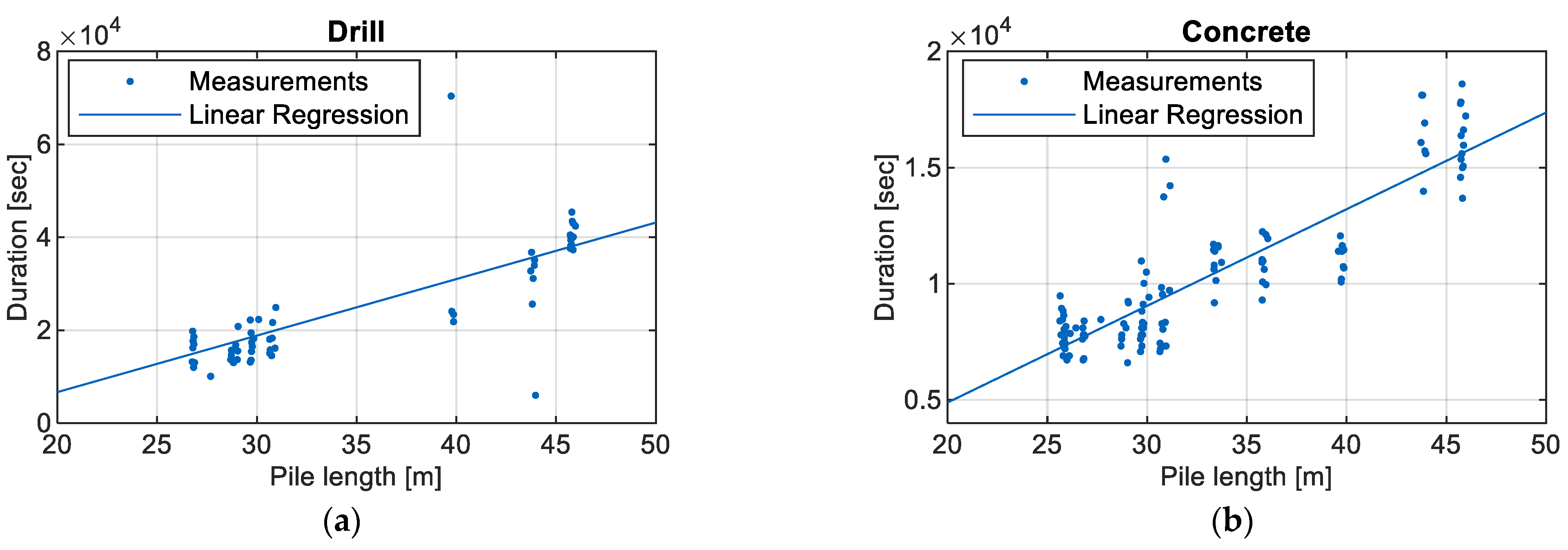
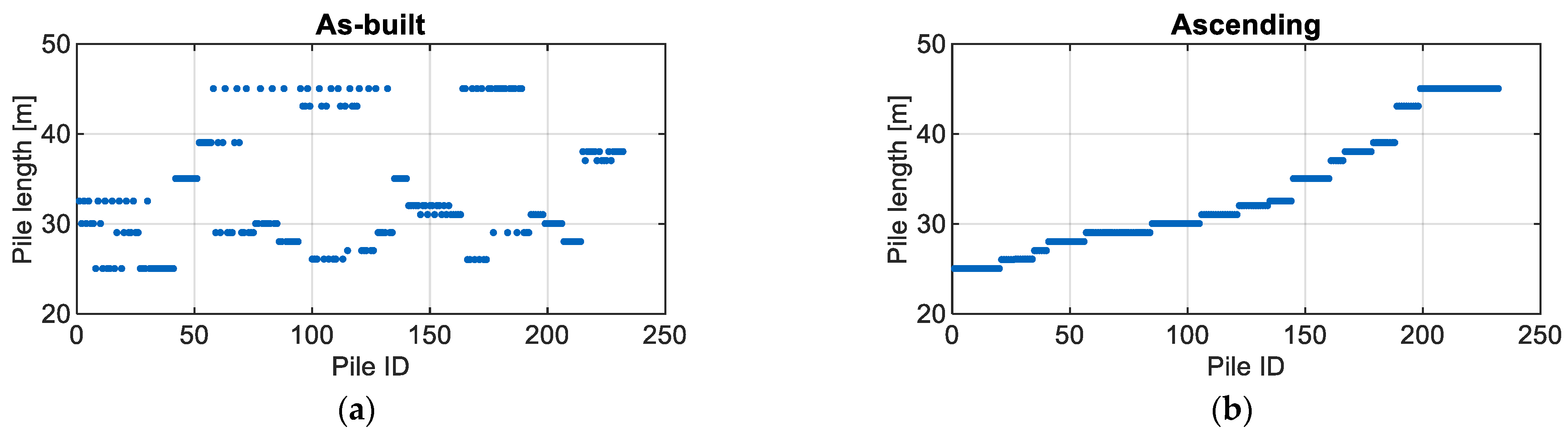
- Production log: Every pile was documented in a handwritten report. This report gave insight into the bored pile sequence and start and end times. Thus, the duration of the following seven subprocesses is derived: (1) drill, (2) idle between drill and reinforce, (3) reinforce, (4) idle between reinforce and install contractor pipe to fill in concrete, (5) install contractor pipe, (6) idle between install contractor pipe and concrete, and (7) concrete. Data from 232 bored piles were analyzed.
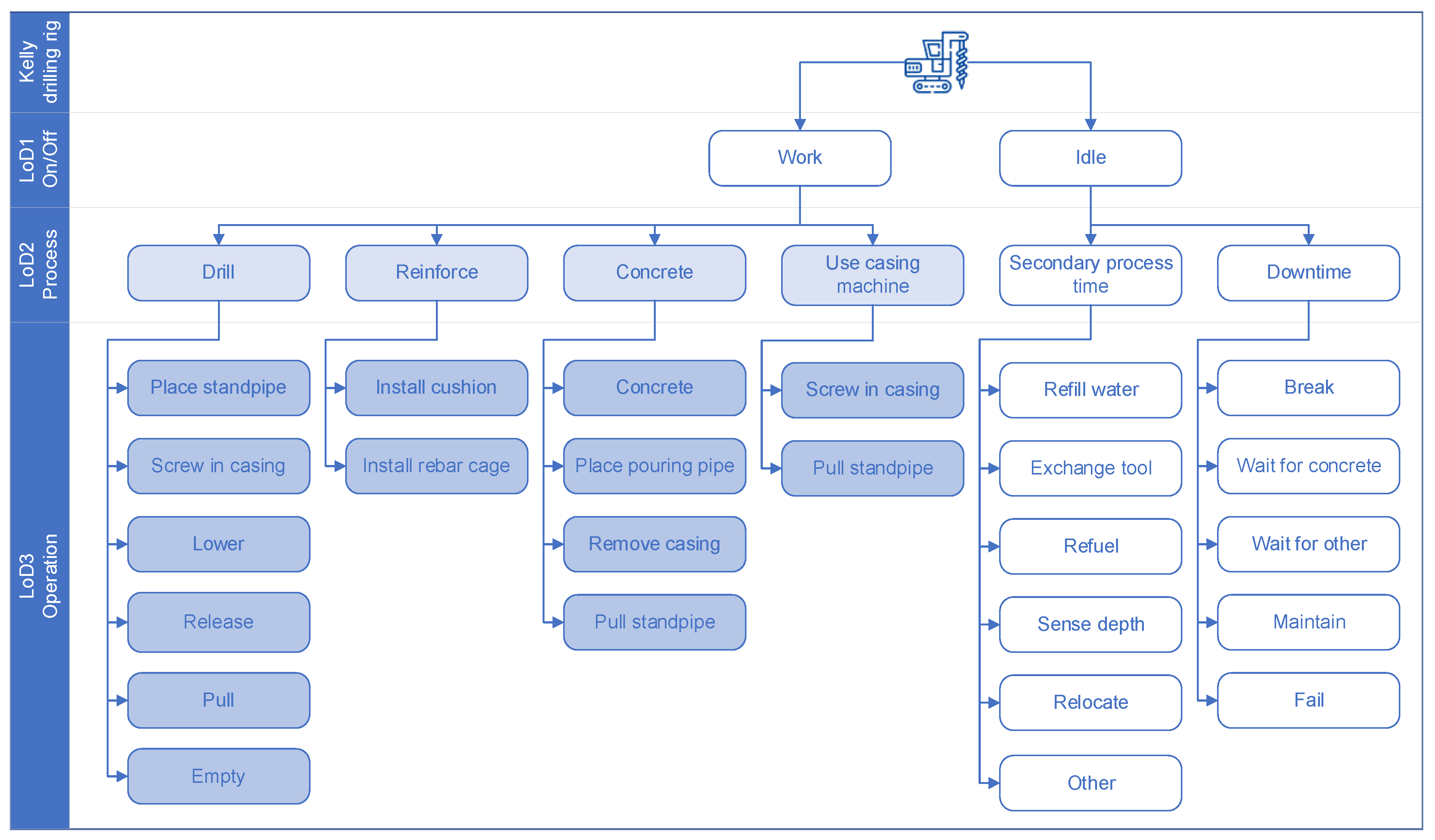
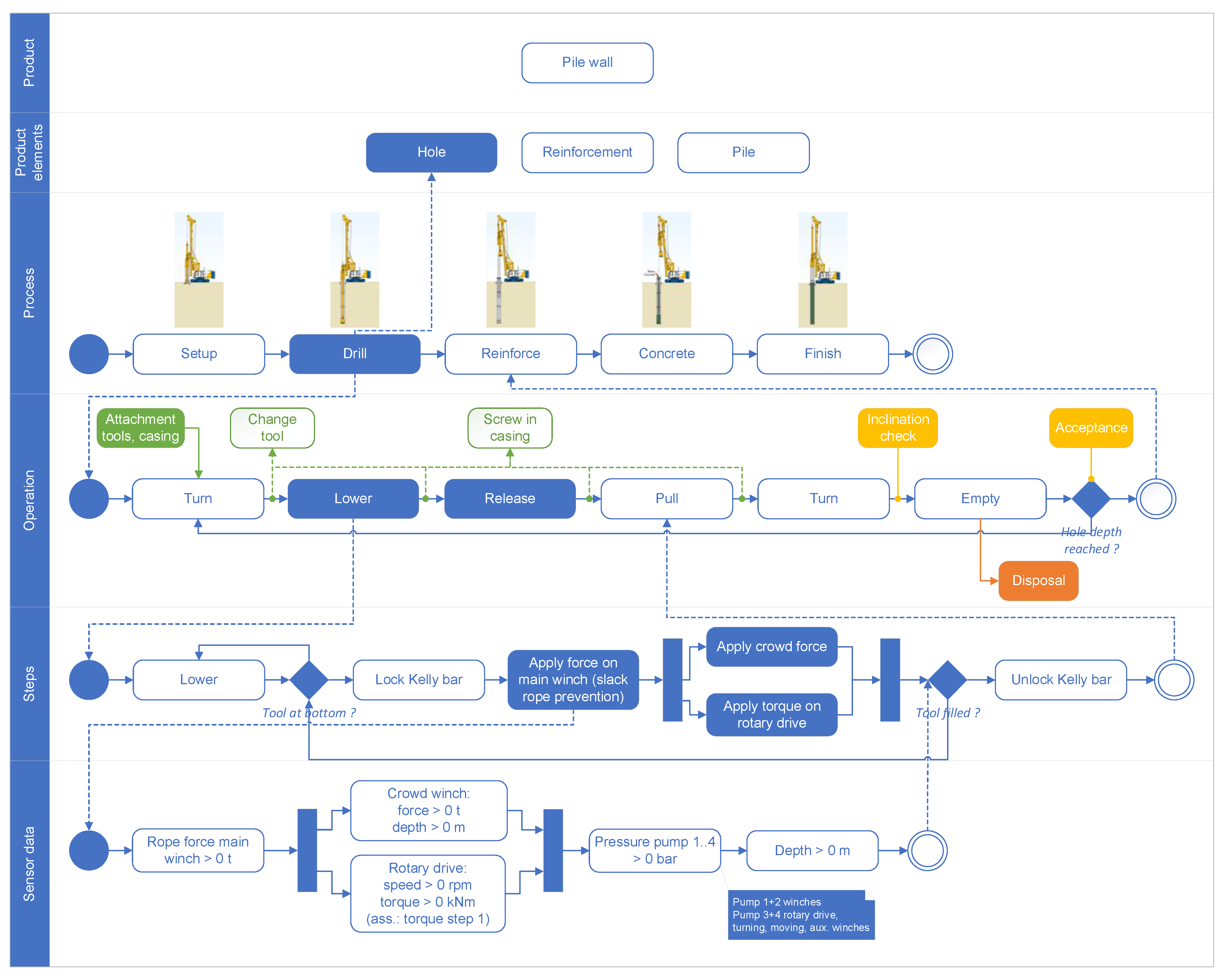
4. Kelly Pile Production System
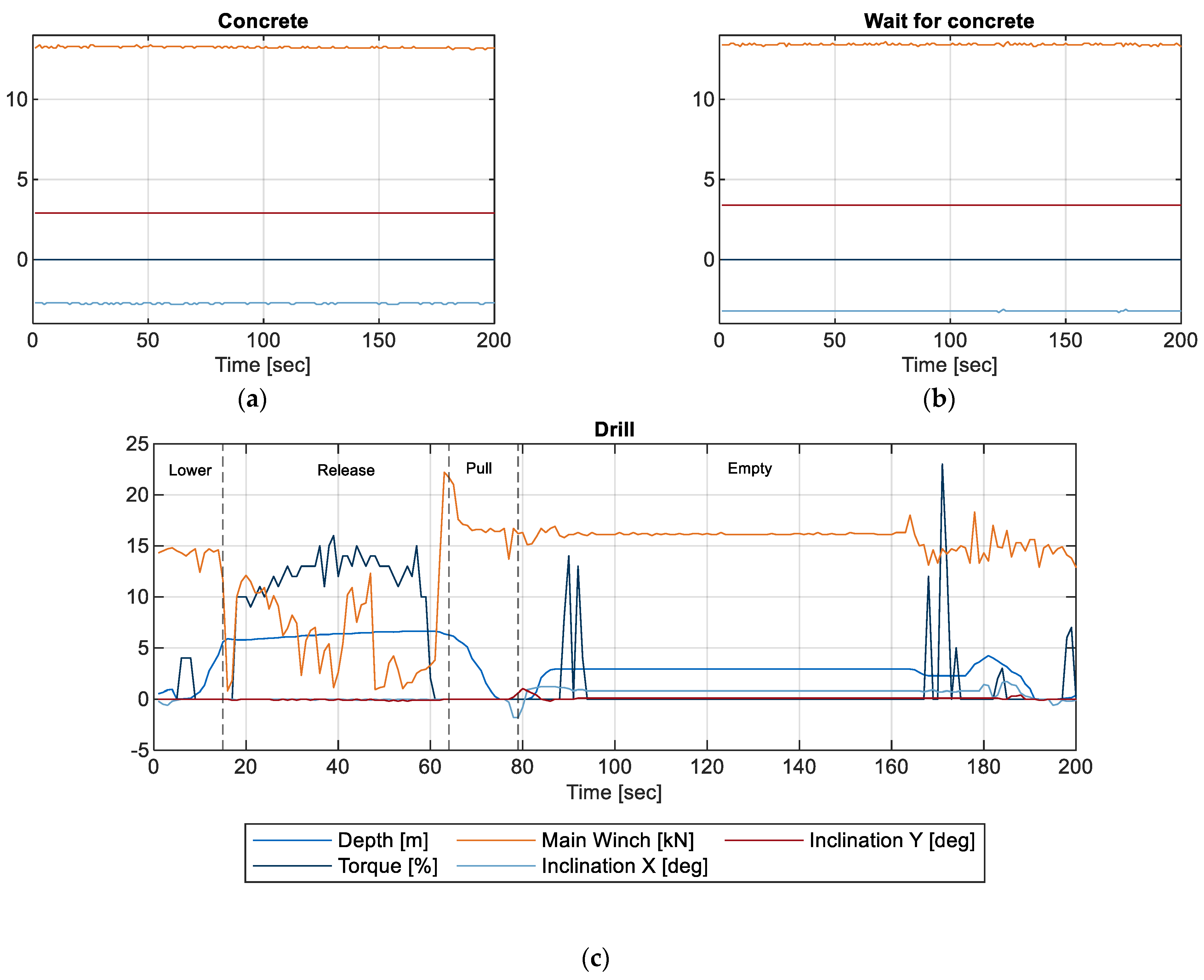
5. Activity Recognition
5.1. Deep Learning Models
5.2. Hierarchical Classification Study
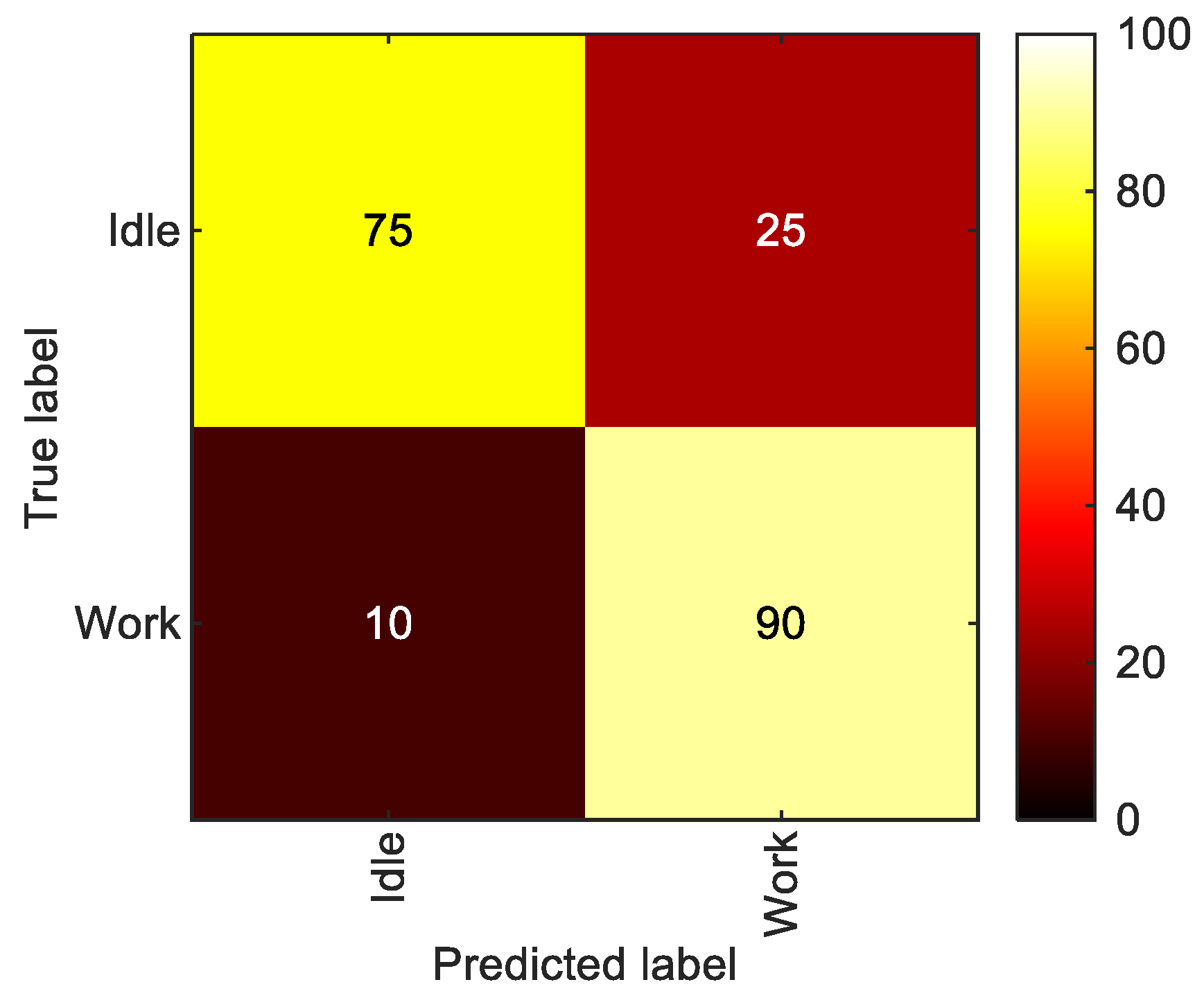
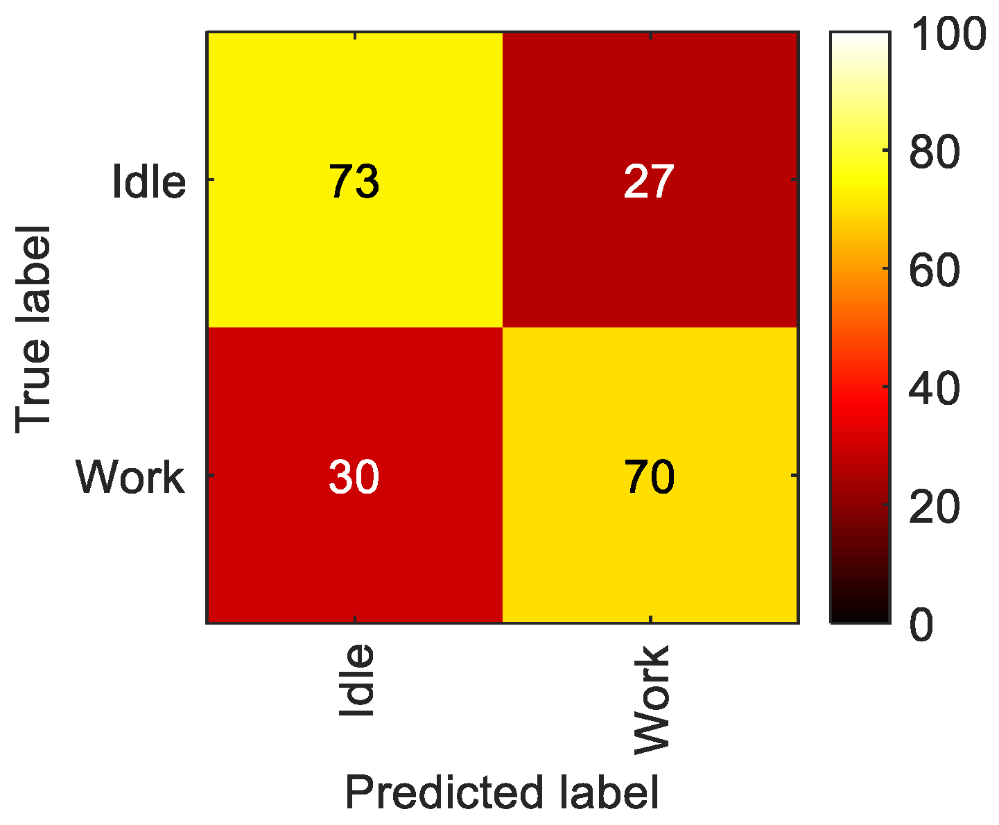
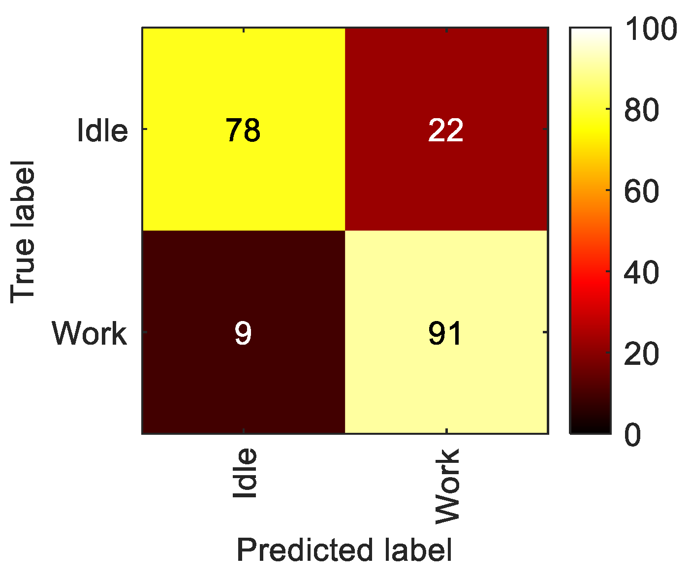
5.2.1. LoD1—Work vs. Idle
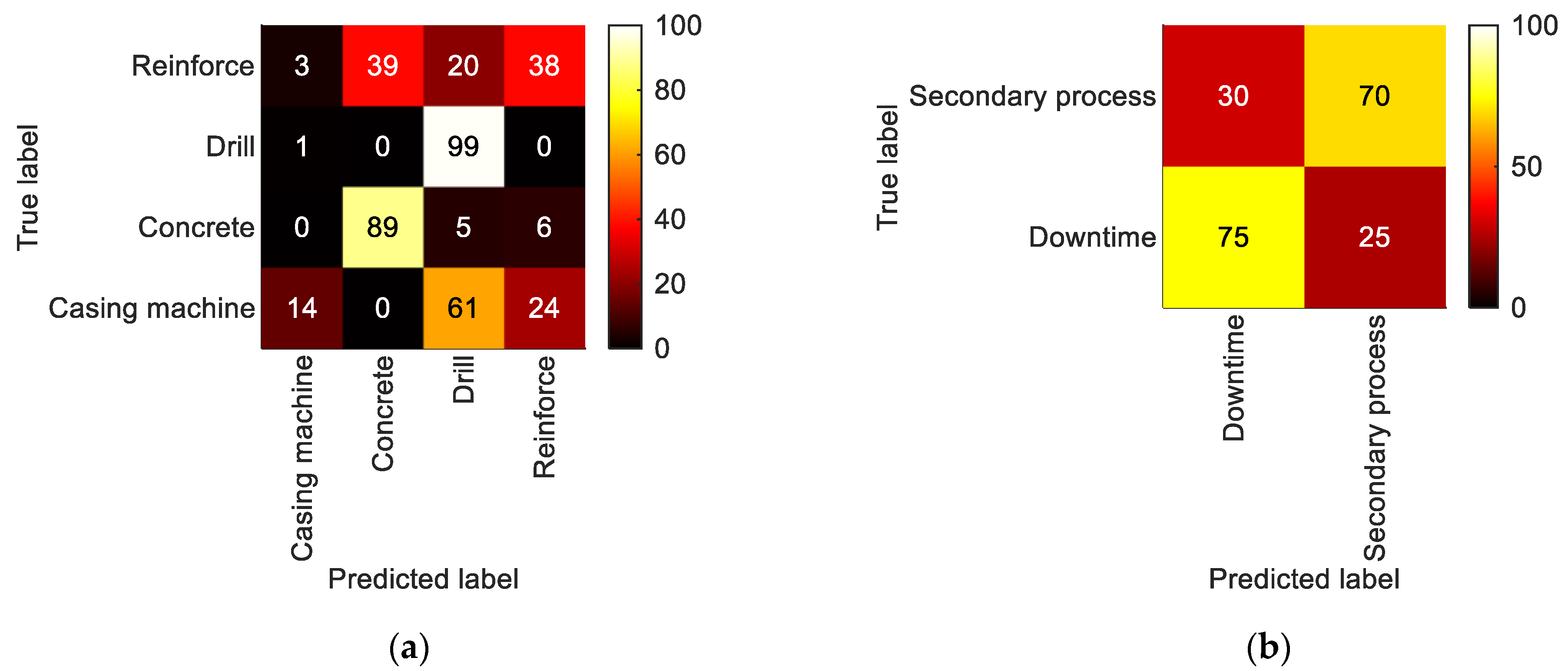
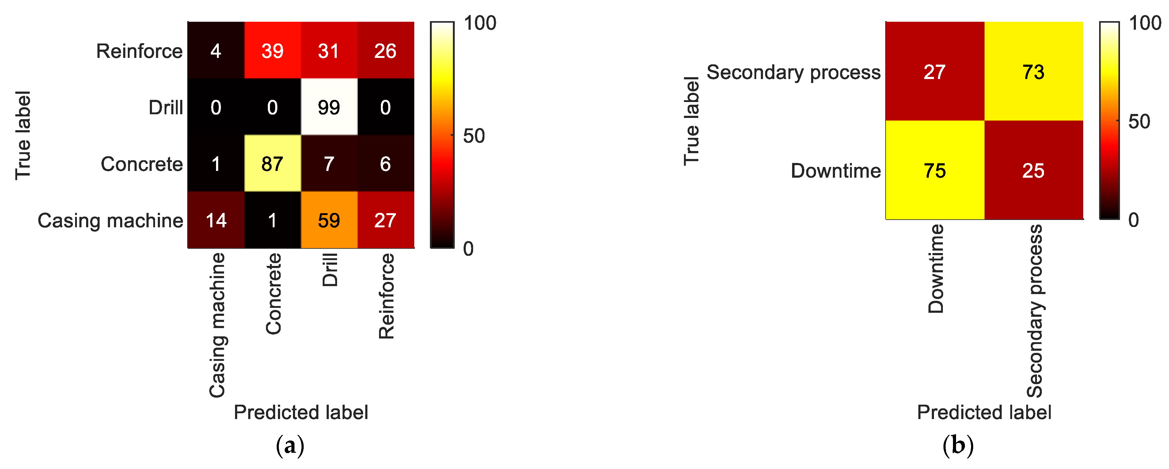
5.2.2. LoD2—Process Steps
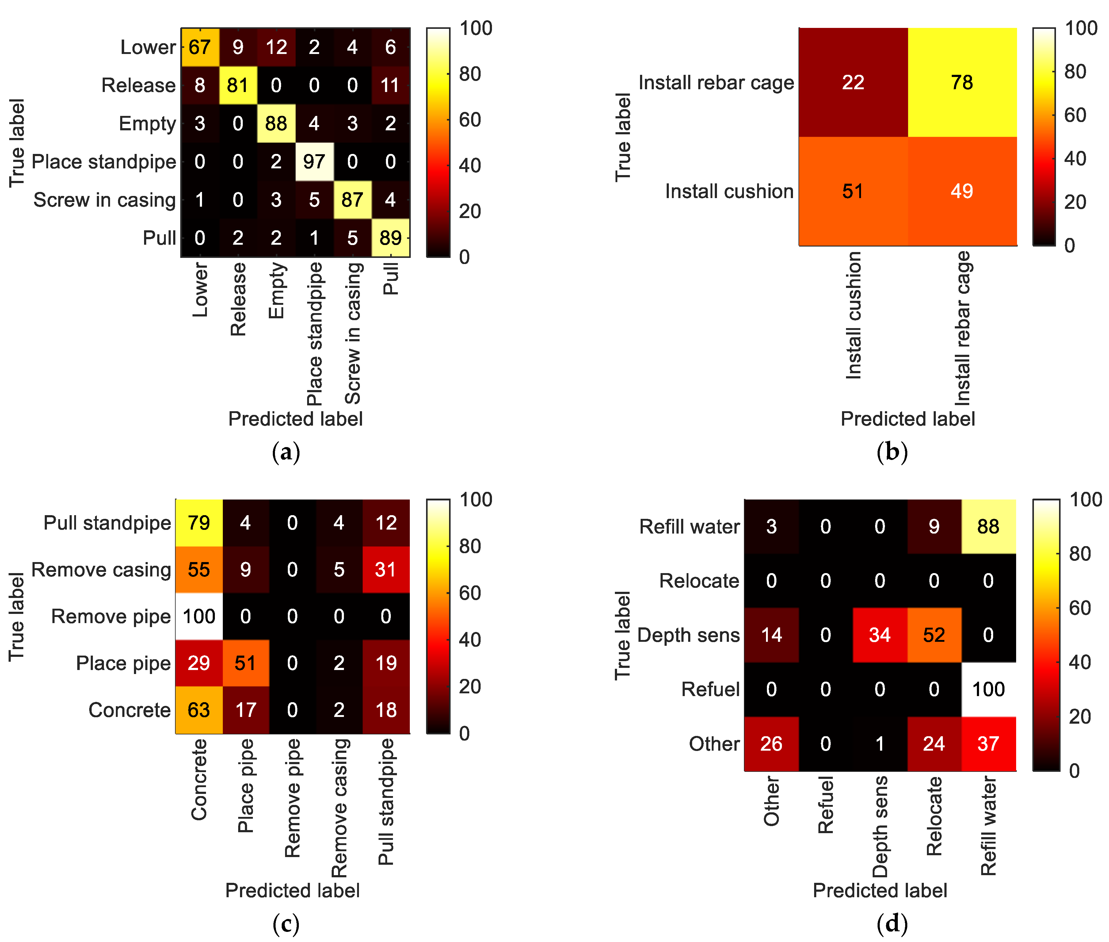
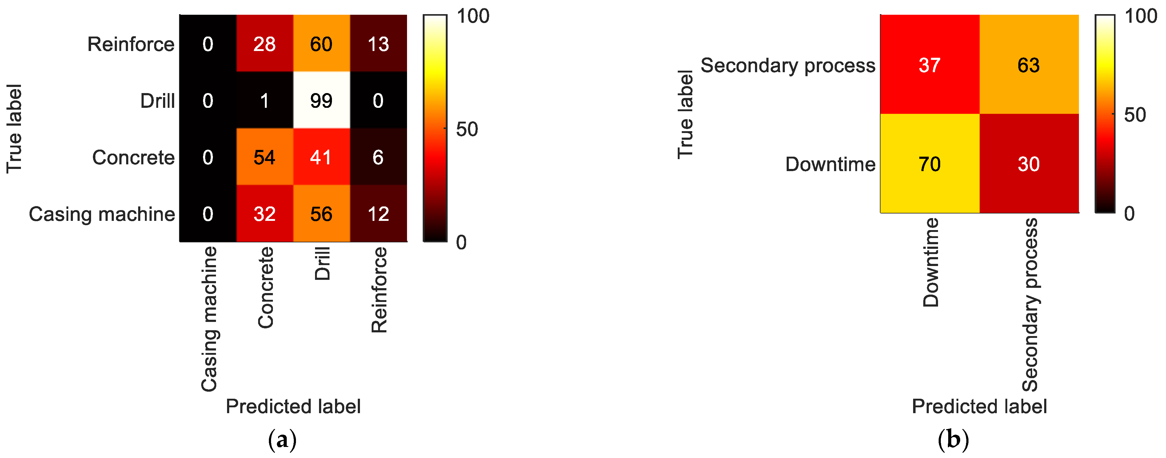
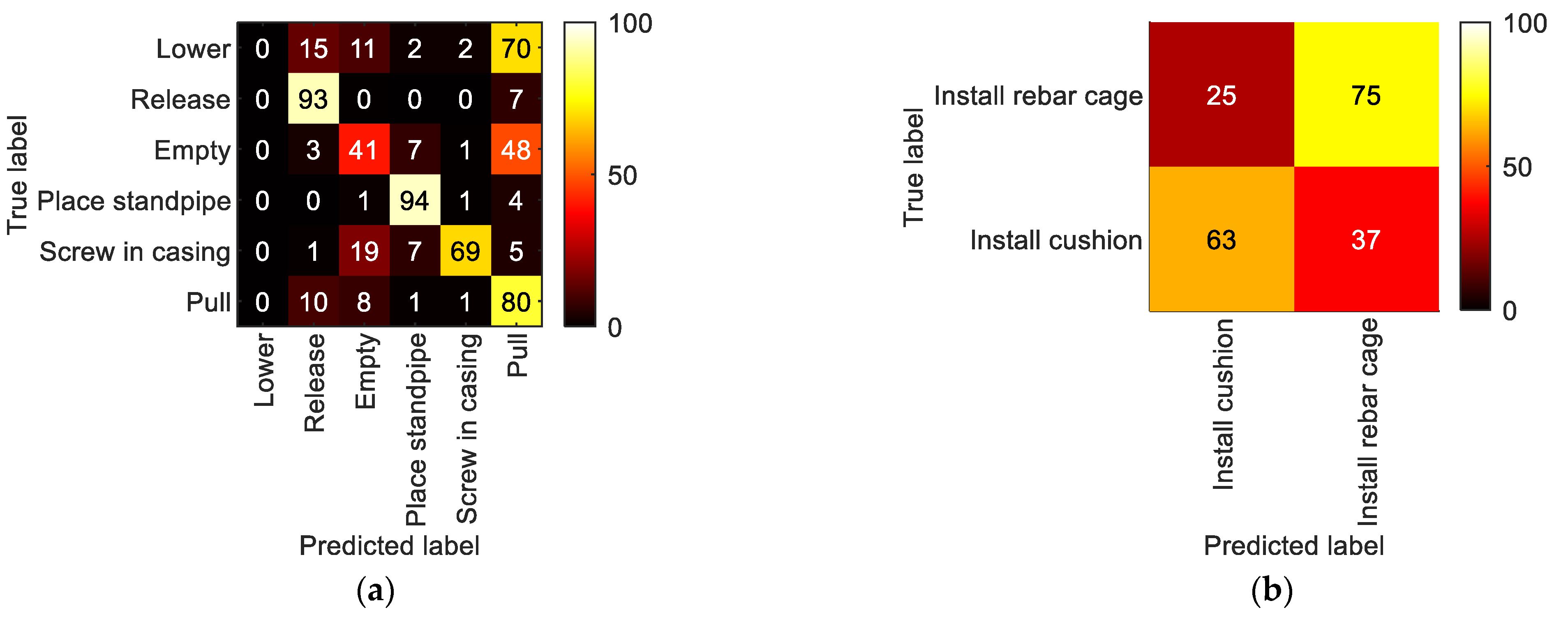
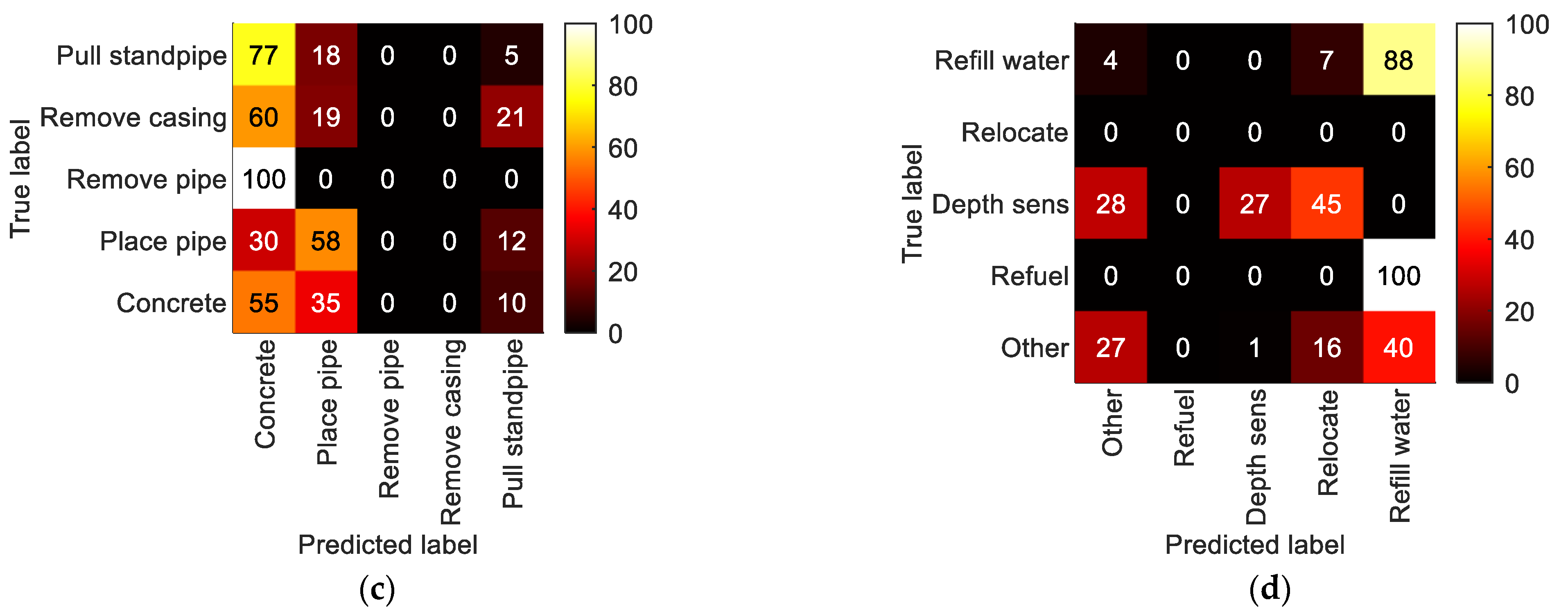
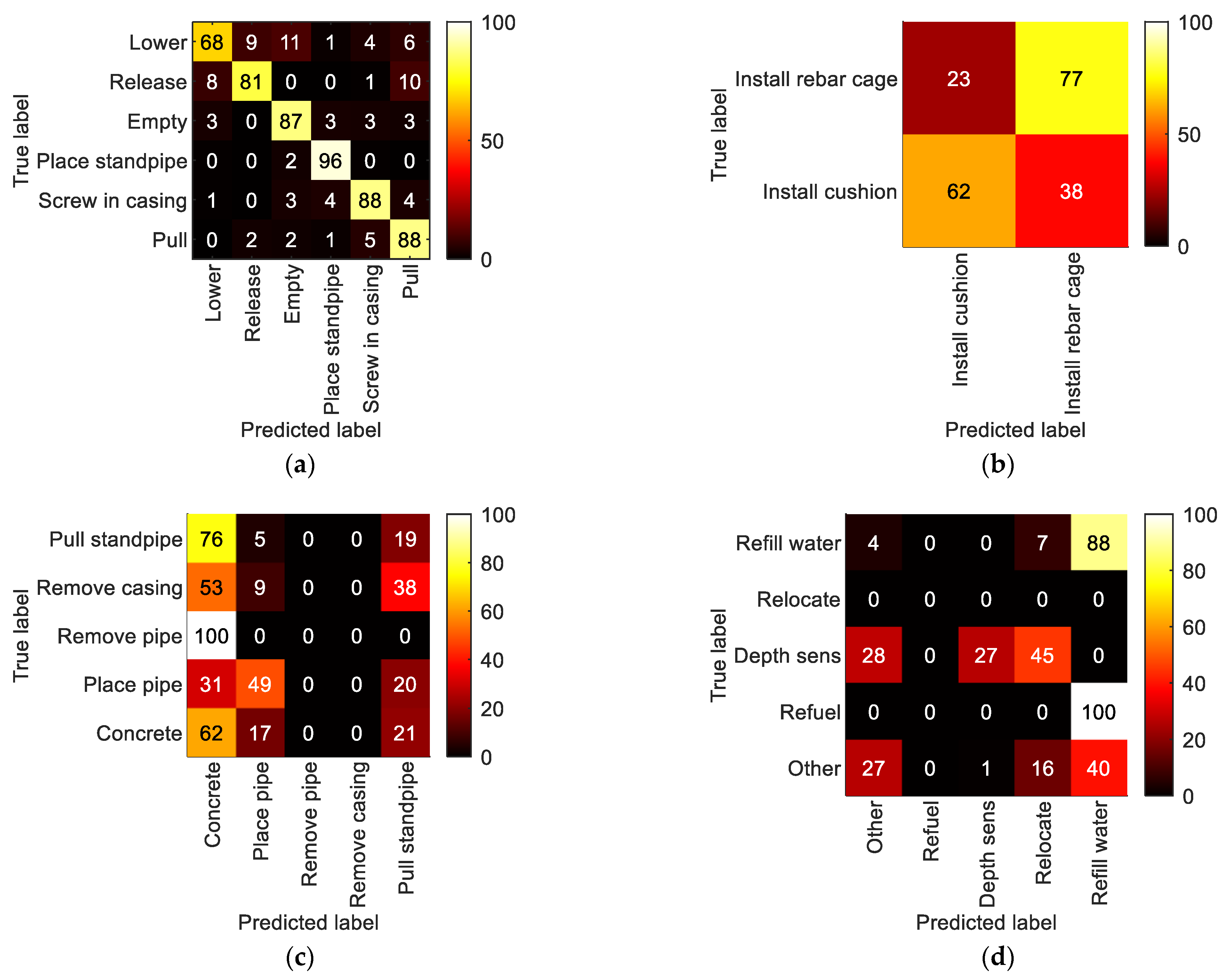
5.2.3. LoD3—Detailed Process Steps
5.3. Conclusion Regarding Activity Recognition
6. Data-Driven DES
6.1. DES Model
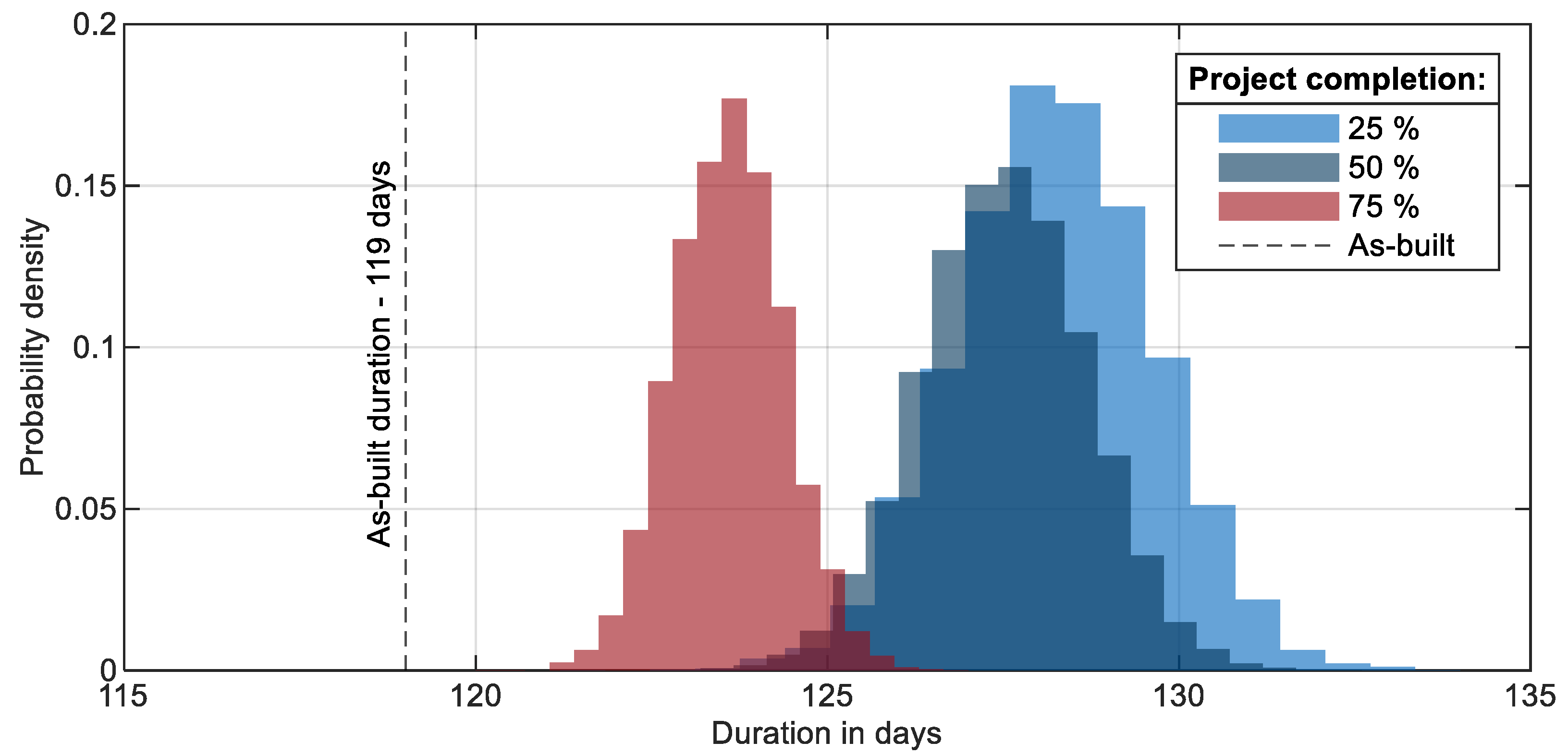
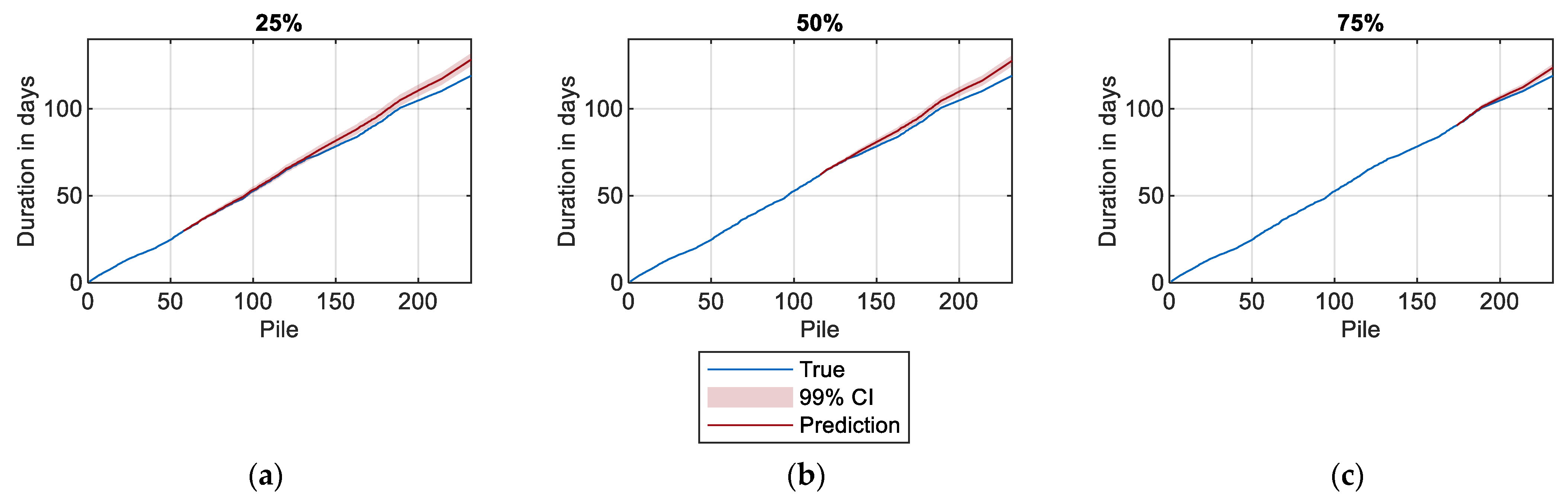
6.2. Forecast Study
6.3. Conclusion Regarding Data-Driven DES
7. Discussion
- RQ1: What impact does production model granularity have on activity recognition?
- RQ2: How does production model granularity affect the application of DTC?
- RQ3: What is needed to adopt production models for DTCs in heavy civil engineering?
8. Conclusions
Author Contributions
Funding
Data Availability Statement
Acknowledgments
Conflicts of Interest
Appendix A


References
- Lasi, H.; Fettke, P.; Kemper, H.-G.; Feld, T.; Hoffmann, M. Industry 4.0. Bus. Inf. Syst. Eng. 2014, 6, 239–242. [Google Scholar] [CrossRef]
- Fuller, A.; Fan, Z.; Day, C.; Barlow, C. Digital Twin: Enabling Technologies, Challenges and Open Research. IEEE Access 2020, 8, 108952–108971. [Google Scholar] [CrossRef]
- Oesterreich, T.D.; Teuteberg, F. Understanding the implications of digitisation and automation in the context of Industry 4.0: A triangulation approach and elements of a research agenda for the construction industry. Comput. Ind. 2016, 83, 121–139. [Google Scholar] [CrossRef]
- Turner, C.J.; Oyekan, J.; Stergioulas, L.; Griffin, D. Utilizing Industry 4.0 on the Construction Site: Challenges and Opportunities. IEEE Trans. Ind. Inf. 2021, 17, 746–756. [Google Scholar] [CrossRef]
- Hu, W.; Lim, K.Y.H.; Cai, Y. Digital Twin and Industry 4.0 Enablers in Building and Construction: A Survey. Buildings 2022, 12, 2004. [Google Scholar] [CrossRef]
- Sacks, R.; Brilakis, I.; Pikas, E.; Xie, H.S.; Girolami, M. Construction with digital twin information systems. Data-Cent. Eng. (DCE) 2020, 1, e14. [Google Scholar] [CrossRef]
- Rashid, K.M.; Louis, J. Integrating Process Mining with Discrete-Event Simulation for Dynamic Productivity Estimation in Heavy Civil Construction Operations. Algorithms 2022, 15, 173. [Google Scholar] [CrossRef]
- Akhavian, R.; Behzadan, A.H. Construction equipment activity recognition for simulation input modeling using mobile sensors and machine learning classifiers. Adv. Eng. Inform. 2015, 29, 867–877. [Google Scholar] [CrossRef]
- Rashid, K.M.; Louis, J. Times-series data augmentation and deep learning for construction equipment activity recognition. Adv. Eng. Inform. 2019, 42, 100944. [Google Scholar] [CrossRef]
- Golparvar-Fard, M.; Heydarian, A.; Niebles, J.C. Vision-based action recognition of earthmoving equipment using spatio-temporal features and support vector machine classifiers. Adv. Eng. Inform. 2013, 27, 652–663. [Google Scholar] [CrossRef]
- Rashid, K.M.; Louis, J. Automated Activity Identification for Construction Equipment Using Motion Data from Articulated Members. Front. Built Environ. 2020, 5, 144. [Google Scholar] [CrossRef]
- Slaton, T.; Hernandez, C.; Akhavian, R. Construction activity recognition with convolutional recurrent networks. Autom. Constr. 2020, 113, 103138. [Google Scholar] [CrossRef]
- Fischer, A.; Liang, M.; Orschlet, V.; Bi, H.; Kessler, S.; Fottner, J. Detecting Equipment Activities by Using Machine Learning Algorithms. In Proceedings of the 17th IFAC Symposium on Information Control Problems in Manufacturing (INCOM 2021), Budapest, Hungary, 7–9 June 2021. [Google Scholar]
- Fischer, A.; Bedrikow, A.B.; Kessler, S.; Fottner, J. Equipment data-based activity recognition of construction machinery. In Proceedings of the 2021 IEEE International Conference on Engineering, Technology and Innovation (ICE/ITMC), Cardiff, UK, 21–23 June 2021; pp. 1–6. [Google Scholar]
- Sherafat, B.; Ahn, C.R.; Akhavian, R.; Behzadan, A.H.; Golparvar-Fard, M.; Kim, H.; Lee, Y.-C.; Rashidi, A.; Azar, E.R. Automated Methods for Activity Recognition of Construction Workers and Equipment: State-of-the-Art Review. J. Constr. Eng. Manag. 2020, 146, 3120002. [Google Scholar] [CrossRef]
- Kritzinger, W.; Karner, M.; Traar, G.; Henjes, J.; Sihn, W. Digital Twin in manufacturing: A categorical literature review and classification. IFAC-PapersOnLine 2018, 51, 1016–1022. [Google Scholar] [CrossRef]
- AbouRizk, S. Role of Simulation in Construction Engineering and Management. J. Constr. Eng. Manag. 2010, 136, 1140–1153. [Google Scholar] [CrossRef]
- Fischer, A.; Li, Z.; Kessler, S.; Fottner, J. Importance of secondary processes in heavy equipment resource scheduling using hybrid simulation. In Proceedings of the 38th International Symposium on Automation and Robotics in Construction (ISARC), Dubai, United Arab Emirates, 4 August 2021; Feng, C., Linner, T., Brilakis, I., Castro, D., Chen, P.-H., Cho, Y., Du, J., Ergan, S., Garcia de Soto, B., Gasparík, J., et al., Eds.; International Association for Automation and Robotics in Construction (IAARC): Pittsburgh, PA, USA, 2021. [Google Scholar]
- Akhavian, R.; Behzadan, A.H. Automated knowledge discovery and data-driven simulation model generation of construction operations. In Proceedings of the 2013 Winter Simulations Conference (WSC), Washington, DC, USA, 8–11 December 2013; pp. 3030–3041. [Google Scholar]
- Kargul, A.; Günthner, W.; Bügler, M.; Borrmann, A. Web based field data analysis and data-driven simulation application for construction performance prediction. Electron. J. Inf. Technol. Constr. 2015, 20, 479–494. [Google Scholar]
- Liu, C.; AbouRizk, S.; Morley, D.; Lei, Z. Data-Driven Simulation-Based Analytics for Heavy Equipment Life-Cycle Cost. J. Constr. Eng. Manag. 2020, 146, 04020038. [Google Scholar] [CrossRef]
- Louis, J.; Dunston, P.S. Methodology for Real-Time Monitoring of Construction Operations Using Finite State Machines and Discrete-Event Operation Models. J. Constr. Eng. Manag. 2017, 143, 04016106. [Google Scholar] [CrossRef]
- Martinez, J.C. Stroboscope: State and Resource Based Simulation of Construction Processes. Ph.D. Dissertation, University of Michigan, Ann Arbor, MI, USA, 1996. [Google Scholar]
- Kim, H.; Bang, S.; Jeong, H.; Ham, Y.; Kim, H. Analyzing context and productivity of tunnel earthmoving processes using imaging and simulation. Autom. Constr. 2018, 92, 188–198. [Google Scholar] [CrossRef]
- Halpin, D.W.; Riggs, L.S. Planning and Analysis of Construction Operations; Wiley: New York, NY, USA, 1992. [Google Scholar]
- Halpin, D.W. An Investigation of the Use of Simulation Networks for Modeling Construction Operations. Ph.D. Dissertation, University of Illinois, Champaign, IL, USA, 1973. [Google Scholar]
- Siemens. Tecnomatix Digital Manufacturing Software. Available online: https://plm.sw.siemens.com/de-DE/tecnomatix/ (accessed on 29 December 2022).
- Fischer, A.; Li, Z.; Wenzler, F.; Kessler, S.; Fottner, J. Cyclic Update of Project Scheduling by Using Telematics Data. IFAC-PapersOnLine 2021, 54, 217–222. [Google Scholar] [CrossRef]
- Fischer, A.; Balakrishnan, G.; Kessler, S.; Fottner, J. Begleitende Prozesssimulation für das Kellybohrverfahren [Accompanying Process Simulation for the Kelly Drilling Process]. In 8. Fachtagung Baumaschinentechnik 2020; TU Dresden: Dresden, Germany, 2020. [Google Scholar]
- Harichandran, A.; Raphael, B.; Mukherjee, A. A hierarchical machine learning framework for the identification of automated construction. ITcon 2021, 26, 591–623. [Google Scholar] [CrossRef]
- Koskela, L. An Exploration towards a Production Theory and Its Application to Construction. Ph.D. Dissertation, Technical Research Centre of Finland, Espoo, Finland, 2000. [Google Scholar]
- Ballard, H.G. The Last Planner System of Production Control. Ph.D. Dissertation, University of Birmingham, Birmingham, UK, 2000. [Google Scholar]
- Koskela, L. Application of the New Production Philosophy to Construction. Stanf. Univ. Tech. Rep. 1992, 72, 39. [Google Scholar]
- Tommelein, I.D. Impact of Variability and Uncertainty on Product and Process Development. In Construction Congress VI; Walsh, K.D., Ed.; American Society of Civil Engineers: Reston, VA, USA, 2000; pp. 969–976. [Google Scholar]
- Ohno, T. Toyota Production System: Beyond Large-Scale Production; Productivity Press: Portland, IN, USA, 1988. [Google Scholar]
- Fischer, A.; Grimm, N.; Tommelein, I.D.; Kessler, S.; Fottner, J. Variety in Variability in Heavy Civil Engineering. In Proceedings of the 29th Annual Conference of the International Group for Lean Construction (IGLC), Lima, Peru, 12–18 July 2021. [Google Scholar]
- Kalsaas, B.T. Further Work on Measuring Workflow in Construction Site Production. In Proceedings of the 20th Annual Conference of the International Group for Lean Construction, San Diego, CA, USA, 18–20 July 2012. [Google Scholar]
- Xu, C.; Chai, D.; He, J.; Zhang, X.; Duan, S. InnoHAR: A Deep Neural Network for Complex Human Activity Recognition. IEEE Access 2019, 7, 9893–9902. [Google Scholar] [CrossRef]
- 1536:2010+A1:2015, 93.020; Execution of Special Geotechnical Work—Bored Piles: German Version EN. DIN Deutsches Institut für Normung: Berlin, Germany, 2015.
- Nübel, K.; Geiss, A.; Sommer, F.; Pielmeier, M.; Heinrich, M.; Rehfeld, B. Produktionsplanung und Produktionssteuerung im Spezialtiefbau [Production planning and production control in special foundation engineering]: Prozessorientierter Ablauf von Bauprojekten im Spezialtiefbau. Bauing. VDI Bautech. 2015, 101–107. [Google Scholar]
- Beiderwellen Bedrikow, A. Equipment Data-Based Activity Recognition of Construction Machinery. Bachelor Thesis, Chair of materials handling, material flow, logistics. Technical University of Munich (TUM), Garching, Germany, 2021. [Google Scholar]
- Hochreiter, S.; Schmidhuber, J. Long short-term memory. Neural Comput. 1997, 9, 1735–1780. [Google Scholar] [CrossRef]
- Ordóñez, F.J.; Roggen, D. Deep Convolutional and LSTM Recurrent Neural Networks for Multimodal Wearable Activity Recognition. Sensors 2016, 16, 115. [Google Scholar] [CrossRef]
- Géron, A. Hands-on Machine Learning with Scikit-Learn, Keras, and TensorFlow: Concepts, Tools, and Techniques to Build Intelligent Systems; O’Reilly Media: Newton, MA, USA, 2019. [Google Scholar]
- Goodfellow, I.; Courville, A.; Bengio, Y. Deep Learning: Das umfassende Handbuch: Grundlagen, aktuelle Verfahren und Algorithmen, neue Forschungsansätze [The Comprehensive Handbook: Fundamentals, Current Methods and Algorithms, New Research Approaches.], 1st ed.; Verlags GmbH & Co. KG: Frechen, Germany, 2018. [Google Scholar]


| Sensor | Unit | Sensor | Unit |
|---|---|---|---|
| Depth | m | Main winch rope speed | cm/min |
| Torque of rotary drive | kNm | Pressure pump 1–4 | bar |
| Speed of rotary drive | Rpm | Torque of Kelly bar | % |
| Main winch rope force | t | Auxiliary winch rope force | t |
| Crowd force | t | Crowd depth | m |
| Casing length | m | Boring threshold | m |
| Status rig | - | Torque steps | - |
| Main winch gear mode | - | Inclination X, Y | deg |
| MLP | DeepConvLSTM | DeepConvBiLSTM | |
|---|---|---|---|
| Architecture | 5xDense-Softmax | 3xCNN–2xLSTM-Softmax | 3xCNN–2xBiLSTM-Softmax |
| Temporal window | no | Overlapping sliding window | Overlapping sliding window |
| Window size | - | 16 s | 16 s |
| Level of Detail (LoD) | Parent Node | MLP | DeepConvLSTM | DeepConvBiLSTM |
|---|---|---|---|---|
| LoD1 | - | 0.83 | 0.84 | 0.83 |
| LoD2 | Work | 0.42 | 0.58 | 0.62 |
| Idle | 0.66 | 0.74 | 0.73 | |
| LoD3 | Drill | 0.59 | 0.85 | 0.85 |
| Reinforce | 0.68 | 0.68 | 0.68 | |
| Concrete | 0.20 | 0.24 | 0.24 | |
| Idle | 0.39 | 0.39 | 0.41 |
| Process | Parameter | 25% | 50% | 75% |
|---|---|---|---|---|
| Drill | Mu | −5.33 × 10⁻¹² | 7.21 × 10⁻¹² | −2.17 × 10⁻¹² |
| Sigma | 7995.83 | 7787.97 | 7090.17 | |
| Slope | 1211.12 | 1216.27 | 1173.93 | |
| Intercept | −16,781.52 | −17,638.90 | −17,837.04 | |
| Idle 1 | Mu | 2.82 × 10⁻¹³ | −7.37 × 10⁻¹³ | −5.02 × 10⁻¹³ |
| Sigma | 3619.61 | 4555.91 | 5119.83 | |
| Slope | −163.18 | −26.71 | −32.85 | |
| Intercept | 12,496.47 | 7209.08 | 7381.52 | |
| Reinforce | Mu | 7.84 × 10⁻¹⁵ | −3.18 × 10⁻¹³ | −6.27 × 10⁻¹³ |
| Sigma | 500.08 | 581.13 | 545.05 | |
| Slope | 105.71 | 83.95 | 75.64 | |
| Intercept | −2299.57 | −1480.55 | −1184.78 | |
| Idle 2 | Mu | 1.39 × 10⁻¹³ | 3.4 × 10⁻¹³ | 1.36 × 10⁻¹³ |
| Sigma | 762.92 | 1869.31 | 1636.55 | |
| Slope | −45.05 | −41.68 | −20.96 | |
| Intercept | 2596.29 | 2519.07 | 1639.18 | |
| Install contractor pipe | Mu | −2.59 × 10⁻¹³ | −3.72 × 10⁻¹³ | −3.55 × 10⁻¹³ |
| Sigma | 785 × 10−1 | 691.22 | 650.05 | |
| Slope | 72.25 | 58.94 | 56.68 | |
| Intercept | −1039.17 | −494.96 | −301.61 | |
| Idle 3 | Mu | 6.27 × 10⁻¹⁴ | −1.09 × 10⁻¹² | −3.35 × 10⁻¹³ |
| Sigma | 2238.13 | 2218.63 | 27,756.29 | |
| Slope | −30.32 | 89.56 | 129.42 | |
| Intercept | 3359.87 | −266.50 | −1134.46 | |
| Concrete | Mu | 0 | −1.11 × 10⁻¹² | −2.7 × 10⁻¹² |
| Sigma | 1407.71 | 1534.68 | 1448.72 | |
| Slope | 267.39 | 415.97 | 436.95 | |
| Intercept | 1505.92 | −3429.70 | −4101.32 |
| Project Completion: | Prediction of Total Pile Production: | |
|---|---|---|
| Ratio of as-Built Data | Mean | Standard Deviation |
| 25% | 128.2 days (+7.76%) | 1.4 days |
| 50% | 127.5 days (+7.14%) | 1.2 days |
| 75% | 123.6 days (+3.86%) | 0.8 days |
| 100% | 119.0 days | - |
Disclaimer/Publisher’s Note: The statements, opinions and data contained in all publications are solely those of the individual author(s) and contributor(s) and not of MDPI and/or the editor(s). MDPI and/or the editor(s) disclaim responsibility for any injury to people or property resulting from any ideas, methods, instructions or products referred to in the content. |
© 2023 by the authors. Licensee MDPI, Basel, Switzerland. This article is an open access article distributed under the terms and conditions of the Creative Commons Attribution (CC BY) license (https://creativecommons.org/licenses/by/4.0/).
Share and Cite
Fischer, A.; Beiderwellen Bedrikow, A.; Tommelein, I.D.; Nübel, K.; Fottner, J. From Activity Recognition to Simulation: The Impact of Granularity on Production Models in Heavy Civil Engineering. Algorithms 2023, 16, 212. https://doi.org/10.3390/a16040212
Fischer A, Beiderwellen Bedrikow A, Tommelein ID, Nübel K, Fottner J. From Activity Recognition to Simulation: The Impact of Granularity on Production Models in Heavy Civil Engineering. Algorithms. 2023; 16(4):212. https://doi.org/10.3390/a16040212
Chicago/Turabian StyleFischer, Anne, Alexandre Beiderwellen Bedrikow, Iris D. Tommelein, Konrad Nübel, and Johannes Fottner. 2023. "From Activity Recognition to Simulation: The Impact of Granularity on Production Models in Heavy Civil Engineering" Algorithms 16, no. 4: 212. https://doi.org/10.3390/a16040212
APA StyleFischer, A., Beiderwellen Bedrikow, A., Tommelein, I. D., Nübel, K., & Fottner, J. (2023). From Activity Recognition to Simulation: The Impact of Granularity on Production Models in Heavy Civil Engineering. Algorithms, 16(4), 212. https://doi.org/10.3390/a16040212