A Tri-Model Prediction Approach for COVID-19 ICU Bed Occupancy: A Case Study

Abstract

The impact of COVID-19 and the pressure it exerts on health systems worldwide motivated this study, which focuses on the case of Greece. We aim to assist decision makers as well as health professionals, by estimating the short to medium term needs in Intensive Care Unit (ICU) beds. We analyse time series of confirmed cases, hospitalised patients, ICU bed occupancy, recovered patients and deaths. We employ state-of-the-art forecasting algorithms, such as ARTXP, ARIMA, SARIMAX, and Multivariate Regression models. We combine these into three forecasting models culminating to a tri-model approach in time series analysis and compare them. The results of this study show that the combination of ARIMA with SARIMAX is more accurate for the majority of the investigated regions in short term 1-week ahead predictions, while Multivariate Regression outperforms the other two models for 2-weeks ahead predictions. Finally, for the medium term 3-weeks ahead predictions the Multivariate Regression and ARIMA with SARIMAX show the best results. We report on Mean Absolute Percentage Error (MAPE), Root Mean Squared Error (RMSE), R-squared ($R^2$), and Mean Absolute Error (MAE) values, for one-week, two-week and three-week ahead predictions for ICU bed requirements. Such timely insights offer new capabilities for efficient management of healthcare resources.

1. Introduction

COVID-19 is a critical and urgent threat to global health [1]. It originates from Wuhan, Hubei province of China. It debuted in late 2019 and spread throughout the world causing a pandemic [2,3]. The causes of its appearance have not yet been determined, although preliminary investigations suggest a zoonotic, possibly bat originated virus [4]. Most countries, including Greece, suffered from this epidemic and applied several policies, such as quarantine, social distancing, travel controls, lockdowns as well as strict monitoring of suspected cases and tracing of confirmed ones in order to mitigate the impact of the disease [5].

As the virus is highly contagious [6], the spread of the disease became unstoppable and met the necessary epidemiological criteria to be declared as a pandemic [7]. Since the outbreak in early December 2019, the number of confirmed COVID-19 cases have exceeded 136 million in 219 countries, and the number of people infected is probably much higher. More than 6.6 million people died from COVID-19 worldwide and in Greece more than 34,000 deaths, up to 20 December 2022 [8,9].

Even though the global response to prepare health systems worldwide is ongoing, it is very difficult to predict the expected number of infected patients and most importantly, the number of patients who require Intensive Care Unit (ICU) admission. Arguably such predictions are critical for resource planning and facility allocation/deployment in hospitals [7,10].

The focus during the pandemic lies within organizational issues, i.e., lack of ventilators, shortage of personal protection equipment, resource allocation, prioritization of limited mechanical ventilation options, and end-of-life care [8]. Efficient diagnosis and prognosis methods are needed to mitigate the burden of the healthcare system and provide patients with the best possible care. Mathematical forecasting models support policy making at the local, state, and national level. They are tools assisting public health decision making and facilitating optimal use of resources to reduce the morbidity and mortality associated with the pandemic [11].

A model for the COVID-19 pandemic developed specifically for China, incorporates several key features including: (1) the importance of the timing and magnitude of the implementation of major government imposed public restrictions designed to mitigate the severity of the epidemic; (2) the importance of both, reported and unreported cases, in interpreting the number of reported cases; and (3) the importance of asymptomatic infectious cases in disease transmission [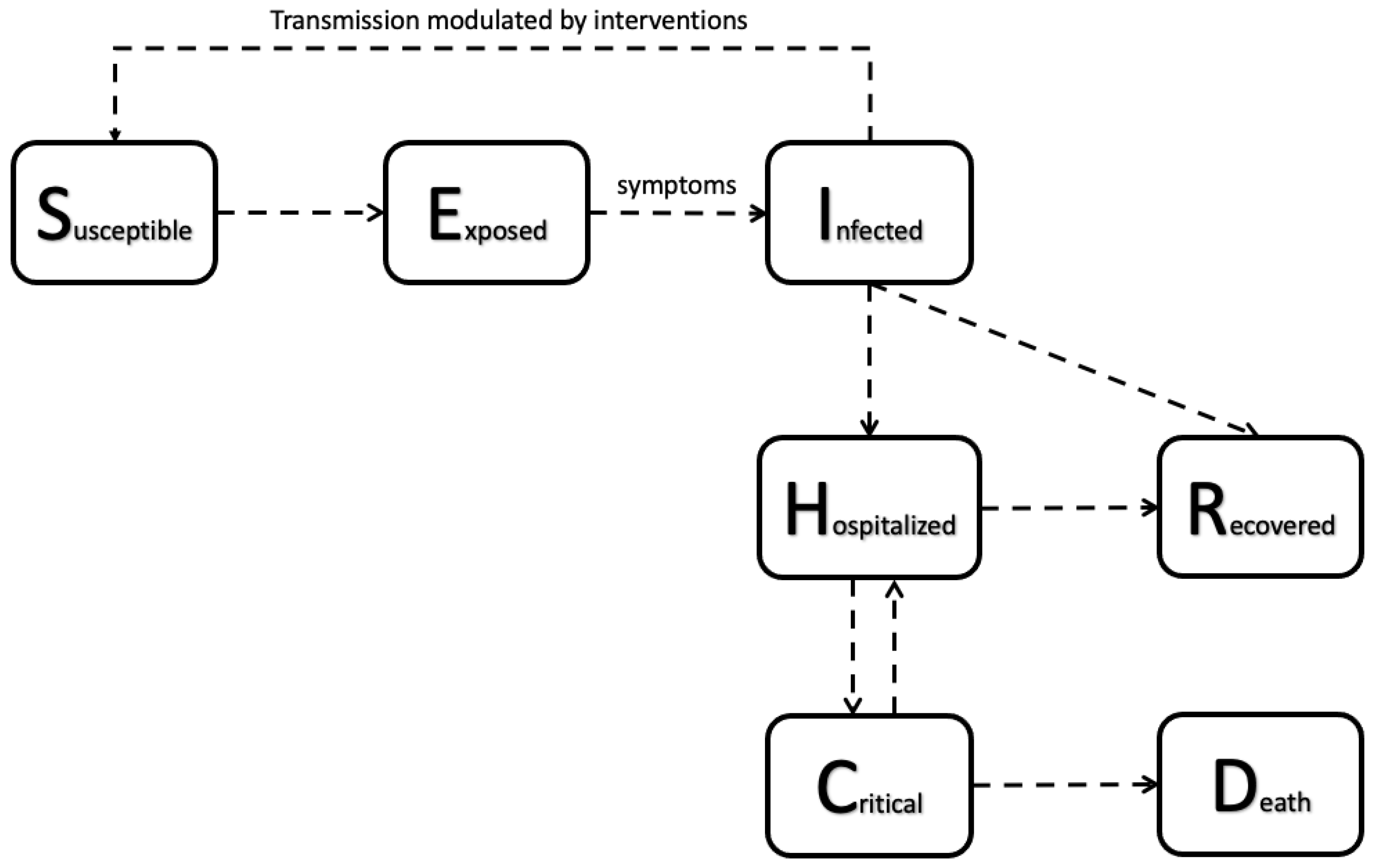12]. Given the same dataset of confirmed cases, high complexity models may not necessarily be more reliable in making predictions, due to the larger number of parameters to be estimated, by comparing standard Susceptible-Infectious-Recovered (SIR) and Susceptible-Exposed-Infectious-Recovered (SEIR) models in predicting the epidemic using the Akaike Information Criterion (Figure 1). Figure 1 refers to hospitalized, critical and death cases while, susceptible is the fraction of susceptible individuals (those able to contract the disease), exposed is the fraction of exposed individuals (those who have been infected but are not yet infectious), infected is the fraction of infective individuals (those capable of transmitting the disease), and recovered is the fraction of recovered individuals (those who have become immune) [2,13,14,15,16].

An attempt to estimate the main epidemiological parameters providing an estimation of the case fatality and case recovery ratios is reported in [17]. Based on the Susceptible-Infectious-Recovered-Dead (SIRD) model, the authors calculated the basic reproduction number ($R_0$), the per day infection mortality and the recovery rates. 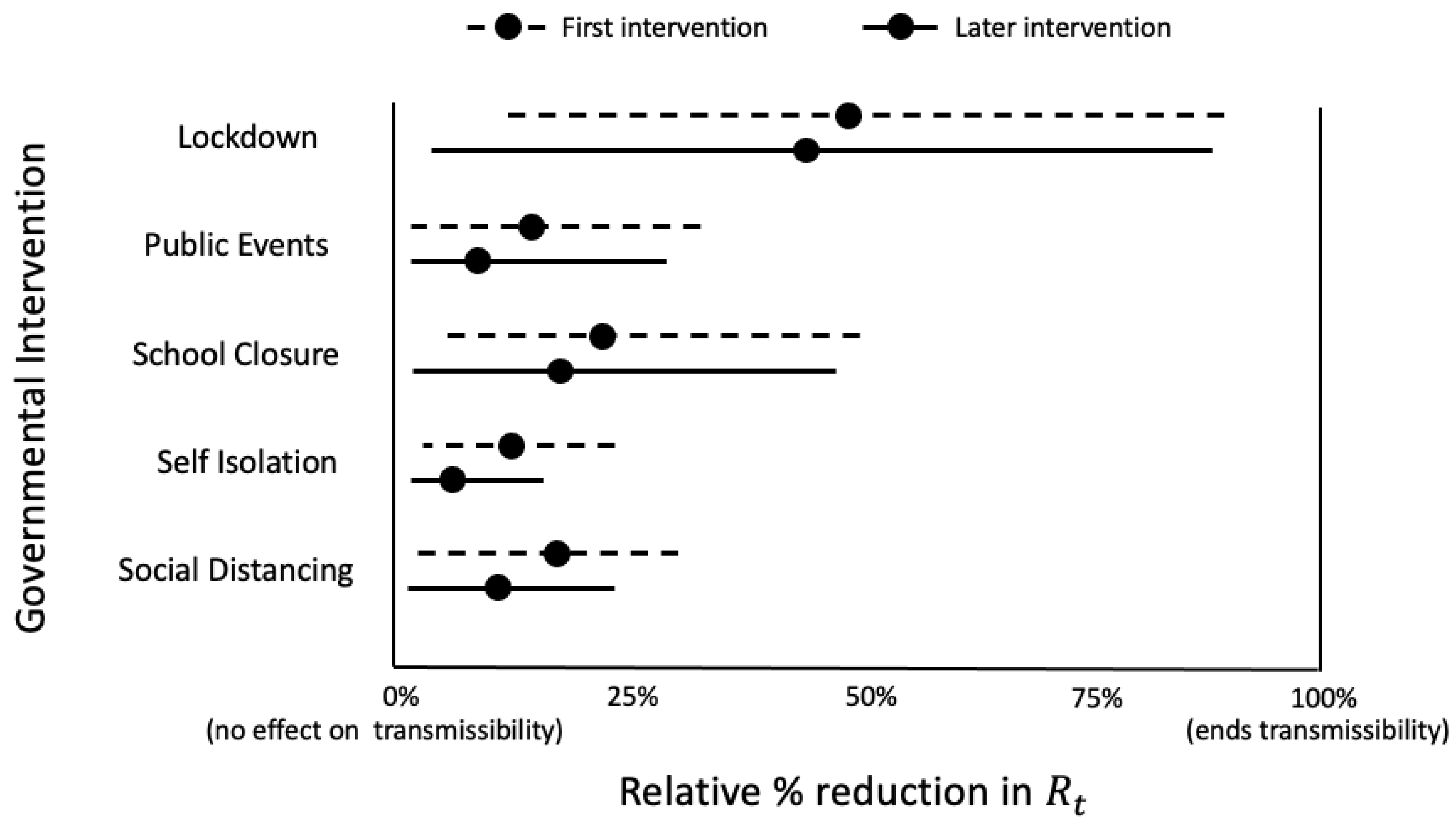The estimated average value for $R_0$ was found to be approximately 2.6 based on confirmed cases and close to 2 based on a second scenario, considering that the number of the infected individuals is much higher than the official numbers [17]. The basic interventions that governments follow to restrict the spread of COVID-19 include five covariates (1) Lockdown, (2) Public Events, (3) School Closure, (4) Self Isolation and (5) Social distancing (Figure 2).

COVID-19 presents a worldwide case study generating new opportunities for demonstrating real-world data mining applications related with epidemics [18,19,20]. The aim of this research is to forecast COVID-19 ICU beds needed in the short to mid-term, with high accuracy and low statistical error. Nevertheless, this kind of epidemiological prediction is ridden with high uncertainty and bias [21,22,23].

We collected time series data for COVID-19 confirmed cases, hospitalised, and intubated patients, ICU bed occupancy, recovered patients and deaths. Our approach is based on state-of-the-art forecasting algorithms (ARTXP, ARIMA, and SARIMAX) and regression models for prediction [24,25,26,27,28,29,30]. We introduce a tri-model time series forecasting approach that yields timely and high precision forecasts, by combining these algorithms into three distinct models, namely ARTXP and ARIMA, ARIMA and SARIMAX, and Multivariate Regression, running simultaneously [31].

The results showcase that this approach predicts ICU beds needs with high accuracy for a one-week ahead, while forecasting accuracy is lower for two weeks and three weeks ahead. In addition, combining ARIMA with SARIMAX produces more accurate results for the majority of the investigated regions in short term 1-week ahead predictions, while Multivariate Regression outperforms the other two models for 2-weeks ahead predictions. Finally, for the medium term 3-weeks ahead predictions the Multivariate Regression and ARIMA with SARIMAX show the best results.

This study aims to forecast COVID-19 ICU needs based on a number of algorithmic models and time series of six variables, including cases, ICU, hospitalized, intubated, recovered patients, and deaths.

The remainder of the article is structured as follows. Section 2 reviews the literature. Section 3 describes the methodology. Section 4 presents and evaluates experimental results. Finally, Section 5 outlines conclusions, along with future work directions.

2. Literature Review

There is a plethora of studies applying prediction models to various COVID-19 related aspects. As we focus on predicting ICU needs, we review recent research examining factors related to ICU requirements during the pandemic.

In [32], the authors developed a prediction model reporting risk scores for ICU admission and mortality for COVID-19. They applied the TRIPOD guideline for developing a multivariable regression model on 641 hospitalized COVID-19 positive patients. Their model yielded 74% accuracy when predicting ICU admission and 83% accuracy when predicting mortality.

In another study, several classification methods were applied to predict level-of-care requirements based on clinical and laboratory data. This information was collected for 2,566 COVID-19 patients and the model resulted in 88% accuracy for hospitalization needs, 87% for ICU care needs, and 86% for mechanical ventilation needs. The authors also produced predictions for Pneumonia severity for ICU care and ventilation with 73% and 74% accuracy, respectively. When predictions were limited to patients with more complex disease, the accuracy of ICU prediction and ventilation was 83% and 82% respectively [9].

A Machine Learning (ML)-based risk prioritization tool was developed to predict imminent (within 24 h) ICU Transfer for Hospitalized COVID-19 patients in [33]. Several time series analyses were used, including vital signs, nursing assessments, laboratory data, and electrocardiograms, as input for training a Random Forest (RF) model. The dataset, that was randomly split into training and test sets using a 70%:30% ratio, consisted of 1987 unique patients who were diagnosed with COVID-19 and admitted to non-ICU hospital units. The research found that the median time to ICU transfer was 2.45 days from the time of admission. Their model performed well compared to actual admissions, with 72.8% sensitivity, 76.3% specificity, 76.2% accuracy, and 79.9% Receiver Operating Characteristic (ROC) Area Under the ROC Curve (AUC).

A similar study was conducted by researchers who developed a Deep Learning prediction of likelihood of ICU admission and mortality for COVID-19 patients, using clinical variables. They collected data including demographics, chronic co-morbidities, vital signs, symptoms and laboratory tests at admission. With the aid of a deep neural model, they predicted ICU admission and mortality with an AUC of 0.780 and 0.844 respectively, whilst the corresponding risk scores yielded an AUC of 0.728 and 0.848, respectively [22,33,34].

In [28,35], researchers attempted to detect early predictive factors upon admission to enhance the management of COVID-19 patients hospitalized in ICUs. The study used data from a hospital in Paris, France, and the authors utilized multivariable logistic regression models; models’ performances, including discrimination and calibration (C-index, calibration curve, Coefficient of Determination ($R^2$), Brier score) were evaluated. Their dataset was about 152 patients hospitalized with positive severe COVID-19 symptoms and the probability of ICU transfer or death was found to be 32% at the 14th day of hospitalization.

Huang et al. [33] developed an external validation of a prognostic multivariable model on admission for hospitalized patients with COVID-19. They collected data from 299 patients for a hospital located at point zero of the pandemic, Wuhan, China (internal evaluation) whilst the external validation was conducted using a retrospective cohort from another Wuhan hospital (145 patients). They utilized a multivariable logistic regression model to predict inpatient mortality for COVID-19 positive patients using 9 variables common with acute respiratory symptoms. In this model they included parameters of age, lymphocyte count, lactate dehydrogenase and $Sp{O}_2$ as independent predictors of mortality, and performed very well in both internal (c = 0.89) and external (c = 0.98) validation.

Another study [12] tried to forecast the spread of COVID-19 and ICU requirements. The authors used data from Kaggle repository and performed regression analysis (ARIMA) in confirmed cases to predict future cases. In addition, using a dataset of 5644 samples, the aid of RF and hard voting, they achieved the highest classification accuracy values close to 98%, and the highest recall value of 98% when predicting whether a COVID-19 patient needs to be admitted to an ICU or semi-ICU room for their treatment.

In addition, a short-term forecast of ICU beds in times of the COVID-19 crisis was provided. The authors concluded that “the use of analytics can provide relevant support for decision making, even with incomplete data and without enough time to fully explore the numerical properties of all available forecasting methods”. Their model combined autoregressive, ML and epidemiological models to provide a short-term forecast of ICU utilization. Their approach demonstrated average forecasting errors of 4% and 9% for one- and two-week horizons, respectively, outperforming several other competing forecasting models [21].

Baas et al. [36] presented a mathematical model that provides a data-driven forecast of the ward and the ICU maximum occupancy of COVID-19 patients in a Dutch hospital. The model is based on the predicted inflow of patients, their Length of Stay (LoS), as well as, transfer of patients between the ward and the ICU.

Heo et al. [37] developed and validated an integer-based score using data from Centres for Disease Control and Prevention (CDC) of South Korea and provided a model for prediction of patients requiring ICU for COVID-19. For a two-month period (from 19 March 2021 until 20 March 2021) the researchers gathered data for 4,663 patients, and developed a model using only clinical variables, resulting in 0.884 AUC for the validation set. Even when seven radiologic and laboratory variables were added (age, sex, initial body temperature, dyspnoea, haemoptysis, history of chronic kidney disease, and activities of daily living), the performance remained almost the same (0.880 AUC).

In [38], an approach for detecting COVID-19 outbreak transmission for Asia Pacific countries utilized time series analysis. It expanded on three different forecasting models, based on Long Short Term Memory (LSTM) networks, Recurrent Neural Network (RNN), and Gated Recurrent Units (GRU), as deep learning techniques. The dataset used, comprised data about the virus spread in the countries under comparison, collected from the WHO website and pre-processed. Their accuracy was close to 90% for the next 10 days.

In [39,40], ML methods such as Decision Trees (DT), Artificial Neural Network (ANN), K-Nearest Neighbour (K-NN), RF, Linear Regression (LR), AdaBoost, Bayesian Boosting, Vote (DT+K-NN), and Vote (DT+K-NN+LR) were employed for ICU mortality prediction. Data about 180 patients were collected from a general hospital (between 2017 and 2018), including demographic information with medical variables, such as Body Mass Index (BMI), stroke, anemia, thrombosis, paraplegia, hypertension. Since there is plenty of research that can detect the possibility of mortality from a medical point of view, in their work they used a different approach that evaluated significant existence of several variables and captured the most important processing scenarios. The findings of the models were compared, and clues were detected about mortality due to underlying diseases, patient age, length of stay, smoking, nutrition, by generating score risks based on results with high accuracy.

The study in [41] referred to India in comparison with other countries, and focused on crucial sectors like the financial, educational, healthcare, industrial, energy, environment, oil market, employment and used exponential smoothing, LR, Holt, Winters as mathematical models to predict the impact on them during the pandemic period and how have lockdowns helped. A comparison for the models was applied for finding similarities between them and to conclude what was the best solution for predicting the impact on these sectors. They concluded that if the growth of a country freezes, the problem of unemployment will increase for these sectors. Results showed that the best performing model was Holt’s and Winter’s.

In another study, a usage of a triple-model forecasting strategy to minimize $R^2$ and maximize MAPE while concentrating on ICU beds was accomplished by the use of ANN, Extreme Gradient Boosting (XGB) and RF algorithms, and showed that ANN had a median $R^2$ value of 99.17% for 21 days while RF and XGB was close with 99.06% and 99.05% respectively [42].

Considering all the aforementioned, this work attempts to predict COVID-19 ICU needs for overall Greece and three distinct Greek areas (Attica, Thessaloniki and Northern Greece) based on several algorithmic models and time series of respected attributes.

3. Research Design

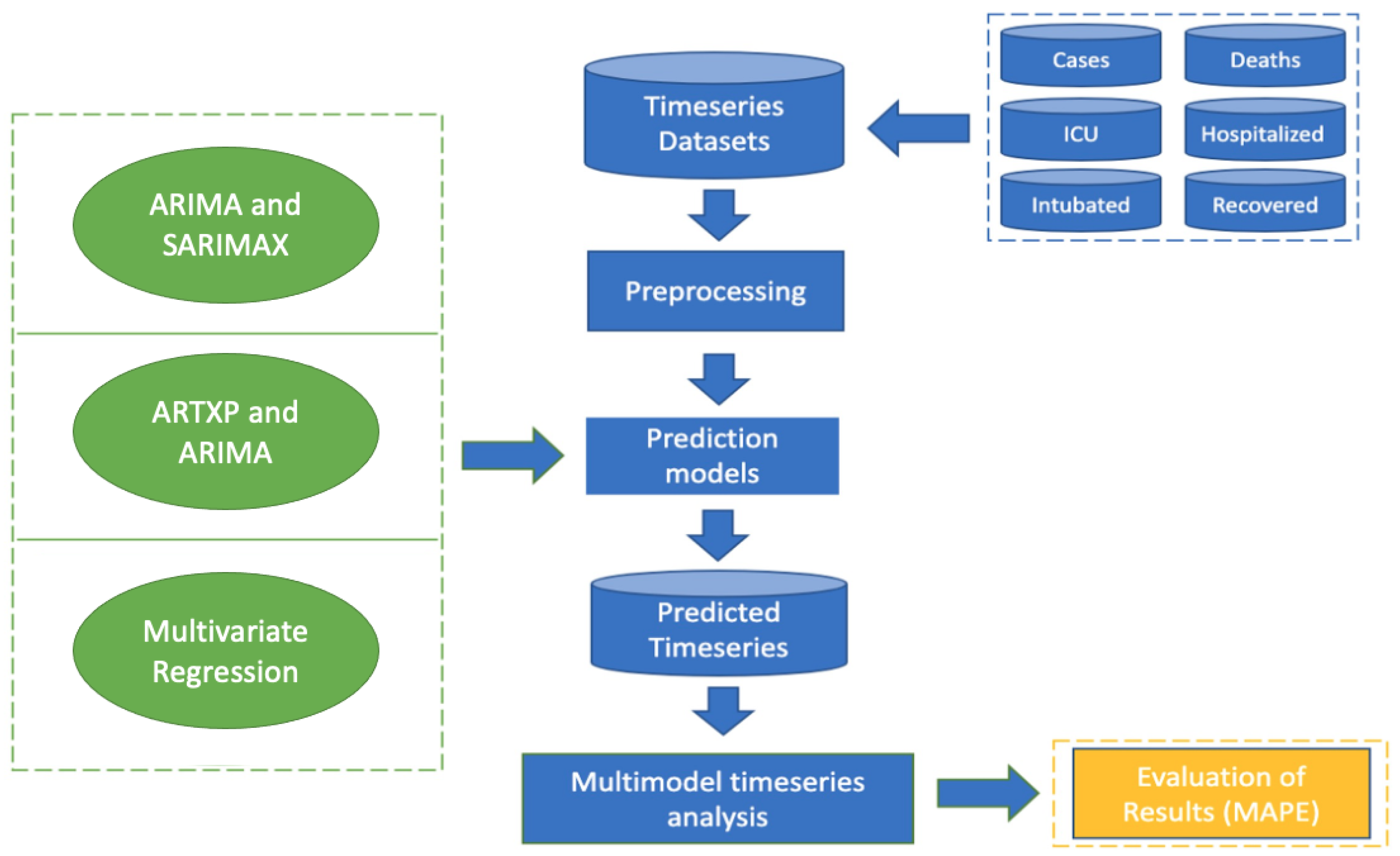
This research attempts to predict COVID-19 ICU needs based on several algorithmic models and time series of six attributes, namely (i) cases, (ii) ICU, (iii) hospitalized, (iv) intubated, (v) recovered patients, and (vi) deaths. These attributes may pose as highly mutable endogenous and exogenous variables, yielding a multi-variable phenomenon. We propose three models (ARTXP and ARIMA, ARIMA and SARIMAX, and Multivariate Regression) as presented in Section 3.2 and benchmark their results. Their purpose is to provide distinct and insusceptible predictions. This section outlines the steps of the proposed methodology. We constructed a database that aggregates and manages time series data (Figure 3). Next, we pre-process data to deal with missing values, noisy data and feature selection methodologies. Each model is executed on the trained time series dataset. The outcome is combined into a unified, tri-model output.

The tri-model output reports on the average values of each model per timestamp on 1-day time resolution for 141 days, from 23 November 2020 until 12 April 2021. Section 4 presents a detailed analysis and evaluates results.

3.1. Data Collection & Pre-Processing

The main data source is the Greek CDC [43] and Ministry of Health [44], but in order to improve the predictions, we also use other data sources providing supplementary attributes for improving forecasting [9]. The selected attributes are: COVID-19 cases, ICU, numbers of hospitalized, intubated, recovered patients and deaths. The time series dataset contains instances from 3 November 2020 until 23 March 2021, while the presentation and evaluation of findings narrate on short and mid-term predictions for COVID-19 related metrics for all the daily announced COVID-19 cases (hospitalized or not) overall Greece and three distinct Greek areas which are Attica, Thessaloniki and Northern Greece (Northern Greece, includes Thessaloniki, Macedonia, Thrace, Epirus, and Thessaly) for that period.

The process of data collection, management and cleansing takes place on a weekly basis. We perform data pre-processing including filling in missing values (0.02% were missing) by manually searching alternative sources to retrieve the actual values or by computing the average between the two closest dates.

Table 1. Periodic forecasting of dataset and model executions.

Variable	Model Execution Date
$d_0$	16 November 2020
$d_1=d_0+x$	23 November 2020
$d_2=d_1+x$	30 November 2020
…	…
$d_{n-1}=d_{n-2}+x$	1 March 2020
$d_n=d_{n-1}+x$	8 March 2020

where $d_{(0\dots n)}$ all the execution dates, from 16 November 2020 up to 8 March 2021, and x = 7.

contains the model execution timestamps related with the forecasting timeslots. We split the timeslots into three intervals, namely one-week (7 days) ahead, two-weeks (14 days) ahead and three-weeks (21 days) ahead. We execute our models on a weekly basis, forecasting daily ICU values for up to 21 days ahead.

3.2. Models & Algorithms

We use a tri-model forecasting approach to establish the best accuracy. Our experimentation process involves three different prediction models, namely ARIMA and SARIMAX, ARTXP and ARIMA, and Multivariate Regression. All models are applied to the same data source, yet utilizing data and parameters varies, as each model according to its process used parameters like periodicity detection, instability sensitivity, complexity penalty, and historic model count.

We implement algorithms and methods by using ML and data mining libraries for classification and regression, such as scikit-learn [45]. These involve scientific libraries, such as Pandas [46], Numpy [47] and Matplotlib [48] for calculus, linear algebra, probabilities, and statistics that enable data analysis, mining and forecasting with Python.

3.2.1. ARIMA and SARIMAX

This model averages the output from ARIMA and SARIMAX algorithmic executions. Next, we present the functionality of these two algorithms and the hyperparameter tuning for our experimentation.

The ARIMA method models the next step in a sequence of observations. It uses a function to linearly calculate the dissimilarity of observations and residual errors of antecedent time steps. A dissimilarity pre-processing step of the sequence and the integration of Autoregression (AR) with Moving Average (MA) models makes the sequence stationary, a process labelled as integration (I). Mathematically, ARIMA can be represented by Equation (1).

$$\Delta y_t=c+{\varphi }_1\Delta y_{t-1}+{\theta }_1{ϵ}_{t-1}+{ϵ}_t$$

(1)

where, c: an intercept of the ARMA (Autoregressive Moving Average) model [49], $\Delta$: the first difference operator and y: the time lags.

For the execution of ARIMA we set the order of AR (p), I (d) and MA (q) models as parameters where, p: the lags in the autoregressive model, d: the differencing/integration order and q: the moving average lags. These parameters are often used to implement AR, MA and ARIMA models.

We exploit ARIMA, when our data are univariate time series, with the existence of trend, yet, with no seasonal components [50]. Initially, we set the order (p, d, q) to (1, 1, 0) i.e., the default parameters set by scikit-learn [45] implementation of ARIMA. Next, since our predictions were running on a weekly basis and as more data were being appended to our initial dataset, we were recalibrating these parameters according to autocorrelation coefficient (ACF) and partial autocorrelation coefficient (PACF) per week. For brevity, we omit reporting these parameter values as it would require showing results for three different models, from the first week of our experimentation until the end.

Next, to examine the existence of seasonality and exogenous variables, we utilized SARIMAX. The exogenous variables are parallel input sequences containing data instances at the time steps of the original (endogenous) data. The exogenous instances stick directly to the model for each time step, while the endogenous time series are modelled differently (e.g., AR, MA). SARIMAX is often used to model the methods involved with exogenous variables, such as ARX, MAX, ARIMAX and many others [49].

Mathematically, SARIMAX can be represented by Equation (2).

$${\varphi }_p\left(L\right){\overline{\varphi }}_p\left(L^s\right){\Delta }^d{\Delta }_s^D{y}_t=A\left(t\right)+{\theta }_q\left(L\right){\overline{\theta }}_Q\left(L^s\right){ϵ}_t$$

(2)

where, ${\varphi }_p\left(L\right)$: the non seasonal autoregressive lag polynomial, ${\overline{\varphi }}_p\left(L^s\right)$: the seasonal autoregressive lag polynomial, ${\Delta }^d{\Delta }_s^D{y}_t$: the time series, differenced d times, and seasonally differenced D times, $A\left(t\right)$: the trend polynomial (including the intercept), ${\theta }_q\left(L\right)$: the non seasonal MA lag polynomial, and ${\overline{\theta }}_Q\left(L^s\right)$: the seasonal MA lag polynomial.

This method is suitable for univariate time series with the existence of trend and/or seasonality and exogenous instances. Similarly, to ARIMA the (p, d, q) parameters set the AR parameters, dissimilarity, and MA parameters. The parameter d is an integer for the integration, p an integer for the AR order and q an integer for the MA order. Otherwise, these parameters are iterables for AR and MA lags for the model. Regarding the seasonal process of SARIMAX we set a (P, D, Q, s) order that models AR, dissimilarities, MA and periodicity, respectively. Parameter D is an integer for the integration process order, P an integer for AR order, Q an integer for MA order or they can be parameters for iterables for AR and/or MA lags for the model, while parameter s gives the periodicity (4 is for quarterly, 12 for monthly data resolution etc.) [49]. After multiple trials for fine hyperparameter tuning, we set the order (p, d, q) to (1, 1, 2) and seasonal order (P, D, Q, s) to (1, 1, 1, 3).

3.2.2. ARTXP and ARIMA

This model utilises ARTXP and ARIMA time series algorithms from MS SQL Server Analysis Services [51]. ARIMA allows the determination of correlations in observations to be taken sequentially in time, as well as the inclusion of error terms in the model. ARTXP and ARIMA support multiplicative seasonality or periodicity generating options for altering the number of possible segments and expected cycles during algorithmic execution. This iterative process increases accuracy. Figure 4 depicts the execution process of this model. ARTXP forecasts the next possible value and ARIMA increases long-term accuracy. As for ARIMA’s parameter tuning, we set the order the same way as explained in Section 3.2.1, since we deal with exactly the same dataset. Each algorithm runs independently before combining results. The combined output is based on historic predictions using actual data. Each forecasted item links with a variable associating it with the historic executions for generating indexing weights.

The combination of algorithmic executions based on indexed weights achieves a cross-prediction process optimised towards the short or medium-term horizon. Depending on the forecasting period and if there is a lockdown in place, we empirically smooth over ARTXP or ARIMA based on historic outputs of this model. In general, when data observations are limited ARTXP performs better. When more data observations are available, ARIMA outperforms ARTXP.

The first step in the ARTXP methodology was to preprocess the time series data related to the spread of COVID-19. Cleaning the data, converting variables, and removing any outliers or abnormalities are all part of this operation. Next, the time series data were divided into segments. For each segment, an autoregressive model fits the data in that segment. The autoregressive models are used to make predictions for future time points. The prediction from the autoregressive models determines which model to use, based on the current state of the time series. This allows the ARTXP model to capture complex, non-linear relationships in the data and to make accurate predictions for future time-points. The performance of the ARTXP model was evaluated (with the metrics reported in this paper) by comparing the predictions with actual values for the spread of COVID-19.

Also, ARTXP tends to report with high accuracy in the short term, i.e., forecasting up to one-week ahead. Although ARIMA is more preferable for predictions beyond a week, it yields a high error rate for the 1st week. For this reason, we utilized a mixed mode prioritizing reporting on ARTXP for the first week and ARIMA for subsequent weeks.

The ARTXP and ARIMA model implements algorithmic optimization by calculating the error rate for each execution iteration. Error rate detects accuracy reduction and enables a mechanism that re-trains the model by automatically introducing coefficients for re-calibrating output values. Model calibration utilizes past error rates.

After experimenting with the effect of error rates on this model’s output, we noticed that by forecasting error rate and supplying it as input to the model, it may improve the model’s performance. In case there are post forecasting actual values available for week n, we perform this process, else we apply error correction based on week $n-1$. Identically, the same process applies for $n+1$ weeks and so on. We calculate the $error\_rate$ (%) on a specific timestamp t according to Equation (3).

$$error\_rat{e}_t=\frac{|Predicte{d}_t-Actua{l}_t|}{Actua{l}_t}\times 100$$

(3)

Finally, the ARTXP and ARIMA model utilizes a variance as a metric for reporting on lower and upper forecasting bounds. Since this model is the most complex among the ones we used, we provide Appendix A clarifying its execution process and parameters involved.

3.2.3. Multivariate Regression

This model takes the average of two predictive scenarios. The first is pessimistic and the second optimistic, following a Multivariate Regression (MR- or multiple LR) model. The MR model is an enhancement of the simple LR equation by increasing the complexity and adding more independent variables in the model. In addition, it considers $R_0$ and lockdown variables. The mathematical formula for this model is presented by Equation (4):

$$ICUbeds=b_0+b_1\times PositiveCases+b_2\times R_0-b_3\times lockdown+e$$

(4)

where, $b_x$: vector/scalar, $PositiveCases$: an independent variable, $R_0$ and $lockdown$: independent variables and e: the statistical error of the equation.

According to Equation (4), the ICU Beds give a forecast based on PositiveCases (dependent variable), $R_0$ and lockdown (which are the independent parameters of the equation) considering the statistical error e and the vector $b_x$ that follows the trend of the phenomenon. Concerning this research study, the output is two datasets of prediction, the pessimistic and the optimistic. Their average is the result of the Multivariate Regression forecasting. Regression analysis is a method which tries to identify and quantify the relationships between multiple variables. The outcome can be adjusted according to the impact of other factors. The advantages of regression are the ease of variable control and isolation by keeping them constant in case of need [52,53,54].

Moreover, the maximum likelihood estimate was utilised for this model in order to maximise the likelihood of the model’s accuracy based on the observed data. Consequently, the optimal values were attained, and this estimate was chosen on the basis of the independent and identical data distribution [55,56].

This method attempts to identify the best fit in their linear multivariate relationship with all variables of the model. Regression is used by quantifying relationships in case of lockdown. When the country was under strict lockdown the independent binary variable $lockdown$ was activated in the equation as a decreasing coefficient. Regression analysis has the capacity to quantify relationships for ICU bed prediction in the short and mid-term. Based on regression analysis by the Multivariate Regression model, there is a relationship between ICU beds (the predicted value), positive COVID-19 cases and the metrics of $R_0$ and lockdown. Experimental trials influenced feature selection with the purpose to eliminate noise of other independent variables that do not affect ICU Beds and finalizing independent parameters ($R_0$ and $lockdown$) of the multivariate model. By selecting different features and checking the correlation of dependent and independent variables separately as for hospitalized, recovered, deaths, $R_0$, means of transport mobility, this study concluded to using positive COVID-19 cases, $R_0$ and the existence of lockdown as independent variables for the regression model.

3.3. Evaluation Metrics

For the validation of results we used MAPE, RMSE, $R^2$ and MAE which refer to the performance of models ARTXP and ARIMA, ARIMA and SARIMAX, and Multivariate Regression as described in Section 3.2. A short description and the mathematical formulation per metric follows.

3.3.1. Mean Absolute Percentage Error (MAPE)

MAPE is a metric that defines the accuracy of a forecasting model. It represents the average of the absolute percentage error of each actual value to assess how close the predicted values were compared with the actual ones. The formula for MAPE is given by Equation (5):

$$MAPE=\frac{100}{i}\sum _{t=1}^i\left|\frac{Actua{l}_t-Forecas{t}_t}{Actua{l}_t}\right|$$

(5)

where, $Actua{l}_t$ is the actual value, $Forecas{t}_t$ the forecasted value, i number of fitted points and t the timestamp.

3.3.2. Root Mean Squared Error (RMSE)

The RMSE is defined as the square root of the average squared difference of actual value and prediction value. RMSE is widely used, since it is measured in the same unit as the target variable. This metric applies more weight to larger errors, given that the impact of a single error on the total is in proportion to its square rather than its magnitude. The formula for RMSE is given by Equation (6):

$$RMSE=\sqrt{\frac{1}{N}\sum _{i=1}^N{(y_i-f_i)}^2}$$

(6)

where $y_i$ is the actual and $f_i$ is the forecasted value for ICUs and N is the amount of values.

3.3.3. R-Squared ($R^2$)

The coefficient of determination ($R^2$) constitutes the comparison of the variance of the errors to the variance of the data to be modeled. It refers to the proportion of variance described by the forecasting model and, unlike other error-based metrics, a higher value means better fit. The formula of $R^2$ is given by Equation (7):

$$R^2=1-\frac{S{S}_{res}}{S{S}_{tot}}=1-\frac{\sum {(y_i-f_i)}^2}{\sum {(y_i-\overline{y})}^2}$$

(7)

where $S{S}_{res}$ is the sum of squares of residuals (errors) and $S{S}_{tot}$ is the total sum of squares (proportional to the variance of the data), $y_i$ is the actual ICUs value, $\overline{y}$ is the mean of the actual values and $f_i$ is the forecasted value for the ICUs.

3.3.4. Mean Absolute Error (MAE)

The calculation of MAE is relatively simple, since it just sums the absolute values of the errors (i.e., the difference between the actual and the predicted value) and then dividing the total error by the number of observations. Compared to other statistical methods, MAE considers all errors having the same weight. The formula of MAE is given by Equation (8):

$$MAE=\frac{1}{N}\sum _{i=1}^N|y_i-f_i|$$

(8)

where $y_i$ is the actual and $f_i$ is the forecasted ICU value and N is the amount of values.

3.4. Limitations

There are various parameters that introduce uncertainty, threatening the validity of our results. For example, parameters related with different demographics and government mitigation actions, changes on traffic regulations, mask policies, social distancing, mini lockdowns in various areas and enforcement of area-specific regulations.

During the COVID-19 spread the Greek government enforced a series of nationwide lockdowns. The first lasted from 22 March 2020 up to 4 May 2020, relaxing special mobility rules in a gradual manner. It was the beginning of the novel COVID-19 virus spread and data were scarce. When more data started to become available, collection and validation involved a quality process of extensive cross checking with other available accredited sources leading to the conception of our proposed forecasting approach [57,58].

In addition, during the first and the second nationwide lockdowns, with the latter lasting from 7 November 2020 until 18 January 2021, Greek citizens complied with the government’s rules and recommendations yielding low levels of mobility, which may be associated with COVID-19 spread. The Greek tactic posed as a paradigm for imitation by other EU countries [59]. These exponential rises or drops in values of observations, such as mobility, were not captured, occasionally resulting in poor forecasting performance [60].

This study reports on a forecasting period from 23 November 2020 until 12 April 2021, engulfing the third nationwide lockdown that lasted from 18 February 2021 until 5 April 2021. Since the datasets improved in terms of observations and validity, the algorithms were recalibrated and performed more efficiently. In addition, the data availability increased, enabling the proposed algorithms to train with bigger dataset and give more accurate results. The main challenge during this period was to consider the forecasting distortion due to lockdowns. We had different kinds of lockdowns and strict government regulations in this time frame. Mini, short-term, long-term, (i.e., days, weeks, months) and distinct lockdowns in various geographical places were applied. In addition, two nation-wide lockdowns took place. This study considers lockdown attribute in a binary form (Yes/No = 1/0), and does not identify hot spots of COVID-19 spread.

COVID-19 outbreaks may also be affected by vaccinations, but during the period of the study the rates were rather low (9% of Greek population fully vaccinated) in order to be considered for our models. In the last three months of the forecasting period (January 2021 to March 2021) more than one million citizens had been vaccinated. We do not consider how this parameter may affect forecasting accuracy [61]. The abovementioned points, generate biases and limitations for the proposed approach to be discussed in Section 5.1, and reduce the accuracy levels of our tri-model approach.

4. Results & Evaluation

The trained forecasting algorithms get as input daily time series including COVID-19 cases, hospitalized, intubated, recovered, ICU patients and deaths. All results were collected to calculate new values, such as error rate to be used for further calculations. For evaluating model accuracy, the average of each metric for all algorithms was compared with actual values.

The forecasting period expands from 23 November 2020 until 12 April 2021, utilizing data from 3 November 2020 until 23 March 2021. We focused on predicting hospitalized patients and more specifically ICU requirements. Confirmed cases may not represent the real number of infected people, as there is a limitation in the number of COVID-19 tests, but official numbers of ICU admissions is a solid data source.

In order to evaluate the accuracy of each method, we used MAPE (

Table 2. MAPE of Predicted vs. Actual ICUs.

Geographical Area	Weeks Ahead Prediction Target	ARTXP and ARIMA (Actual/3d) (%)	ARIMA and SARIMAX (Actual/3d) (%)	Multivariate Regression (Actual/3d) (%)	All Models’ Average (Actual/3d) (%)
Thessaloniki	1	12.22/11.36	13.35/12.41	13.09/11.88	11.53/10.69
	2	26.46/25.12	27.86/25.74	22.63/20.77	21.80/19.53
	3	41.97/39.89	32.72/31.82	35.95/34.17	29.80/27.95
Northern Greece	1	17.26/15.92	9.36/7.99	9.74/8.12	10.88/9.12
	2	32.05/29.52	21.80/19.40	18.80/16.50	20.61/17.98
	3	52.56/49.56	34.44/33.77	30.05/29.18	31.94/30.94
Greece	1	8.15/7.51	5.05/4.69	5.53/4.80	5.45/4.73
	2	16.73/15.48	13.90/13.11	9.73/8.52	11.40/10.24
	3	24.15/23.28	23.49/22.87	21.32/19.80	18.81/17.86
Attica	1	7.07/6.47	5.83/4.60	7.92/6.26	6.26/4.79
	2	14.76/13.79	12.20/10.87	14.07/12.74	12.14/11.07
	3	23.96/23.50	17.63/16.69	21.42/20.19	18.55/17.81
Overall Average		23.11/21.78	18.14/17.00	17.52/16.08	16.60/15.23

), RMSE (

Table 3. RMSE of Predicted vs. Actual ICUs.

Geographical Area	Weeks Ahead Prediction Target	ARTXP and ARIMA (Actual/3d) (ICUs)	ARIMA and SARIMAX (Actual/3d) (ICUs)	Multivariate Regression (Actual/3d) (ICUs)	All Models’ Average (Actual/3d) (ICUs)
Thessaloniki	1	16.88/16.00	16.81/15.25	15.98/14.17	16.56/15.14
	2	35.58/33.38	33.13/30.13	25.03/22.33	31.25/28.61
	3	49.57/46.88	34.97/33.03	36.28/33.86	40.27/37.92
Northern Greece	1	41.96/39.20	20.54/16.86	76.28/74.66	46.26/43.57
	2	70.25/65.88	48.01/43.60	39.26/35.50	52.51/48.33
	3	107.01/102.87	66.60/64.29	59.29/56.03	77.63/74.40
Greece	1	54.47/52.32	32.71/28.12	34.14/28.91	40.44/36.45
	2	100.46/94.69	73.40/69.97	61.64/55.47	78.50/73.38
	3	139.97/134.86	124.58/122.09	113.60/107.02	126.05/121.32
Attica	1	19.87/19.32	18.17/15.21	23.29/18.08	20.44/17.54
	2	46.40/45.08	35.21/32.10	42.24/37.27	41.28/38.15
	3	83.28/82.27	55.60/52.41	69.02/63.98	69.30/66.22
Overall Average		63.81/61.06	46.64/43.59	49.67/45.61	53.37/50.09

), $R^2$ (

Table 4. $R^2$ of Predicted vs. Actual ICUs.

Geographical Area	Weeks Ahead Prediction Target	ARTXP and ARIMA (Actual/3d) (%)	ARIMA and SARIMAX (Actual/3d) (%)	Multivariate Regression (Actual/3d) (%)	All Models’ Average (Actual/3d) (%)
Thessaloniki	1	94/95	94/95	91/93	93/94
	2	86/88	85/88	83/88	85/88
	3	64/70	69/72	56/62	63/68
Northern Greece	1	91/92	97/98	96/97	95/96
	2	76/79	91/94	85/87	84/87
	3	44/49	77/79	69/72	63/66
Greece	1	89/90	96/98	96/97	94/95
	2	68/71	87/89	87/90	81/83
	3	45/48	70/72	58/62	58/61
Attica	1	99/99	98/99	98/98	98/99
	2	93/94	97/97	96/96	95/96
	3	88/89	92/93	91/92	90/91
Overall Average		78/80	88/89	84/86	83/85

) and MAE (

Table 5. MAE of Predicted vs. Actual ICUs.

Geographical Area	Weeks Ahead Prediction Target	ARTXP and ARIMA (Actual/3d) (ICUs)	ARIMA and SARIMAX (Actual/3d) (ICUs)	Multivariate Regression (Actual/3d) (ICUs)	All Models’ Average (Actual/3d) (ICUs)
Thessaloniki	1	11.67/10.26	12.52/11.59	12.19/11.29	12.13/11.04
	2	27.37/25.63	25.53/23.37	19.26/17.71	24.05/22.24
	3	38.41/36.59	27.71/26.51	27.88/26.21	31.33/29.77
Northern Greece	1	33.38/30.49	15.19/12.27	31.90/28.99	26.83/23.92
	2	58.37/54.49	37.95/34.32	32.58/29.33	42.96/39.38
	3	84.82/81.08	55.24/53.57	50.06/47.92	63.37/60.86
Greece	1	40.10/37.28	22.76/20.72	26.81/23.30	29.89/27.10
	2	81.79/76.25	63.37/59.13	47.11/41.28	64.09/58.89
	3	112.47/107.98	104.12/100.45	100.24/93.55	105.61/100.66
Attica	1	17.91/17.45	15.00/11.94	20.27/15.88	17.73/15.09
	2	41.30/38.79	32.80/29.29	36.20/32.49	36.77/33.52
	3	74.00/72.26	49.78/46.48	61.00/56.14	61.59/58.29
Overall Average		51.80/49.04	38.50/35.80	38.79/35.34	43.03/40.06

) for the predicted versus the actual values for this period, for four separate geographical regions of interest (Thessaloniki, Northern Greece, Attica and Greece) and for 1–3 weeks ahead. In these tables we also include the 3-day MA values per metric, providing a more reliable outlook on prediction error, given that the 3-day MA method unravels data collection lags attributed to weekends or national holidays.

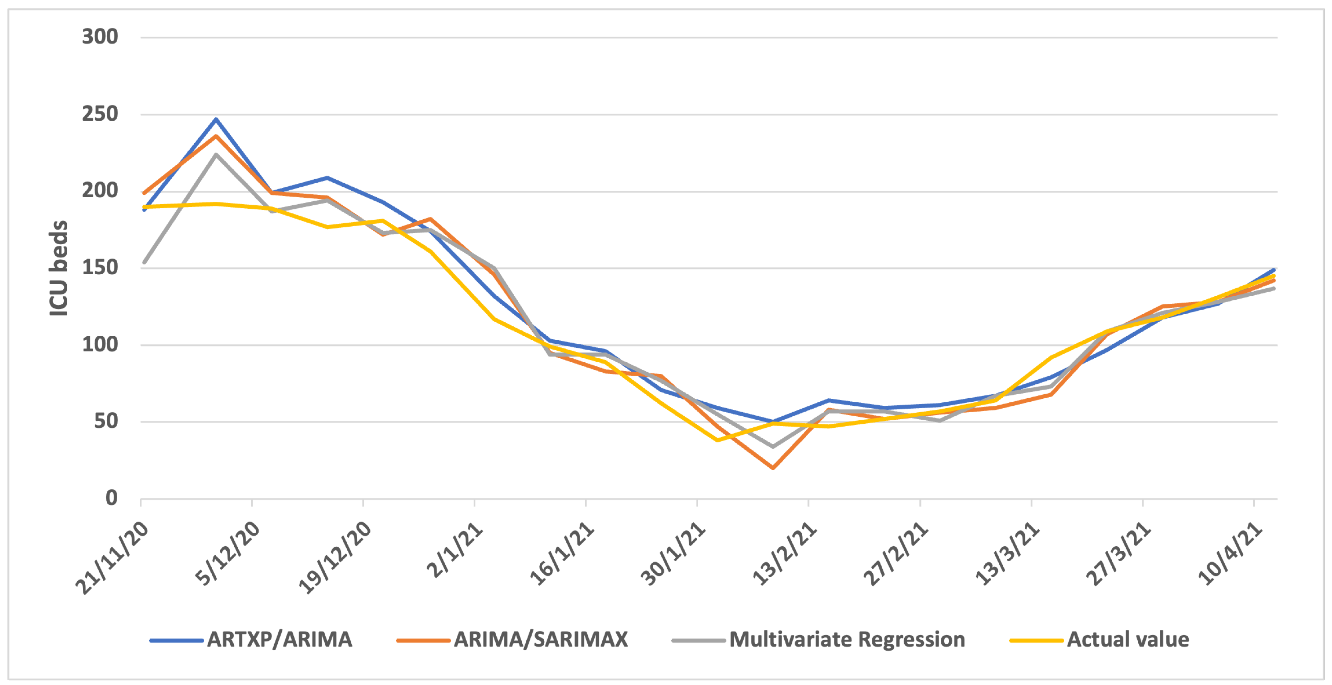
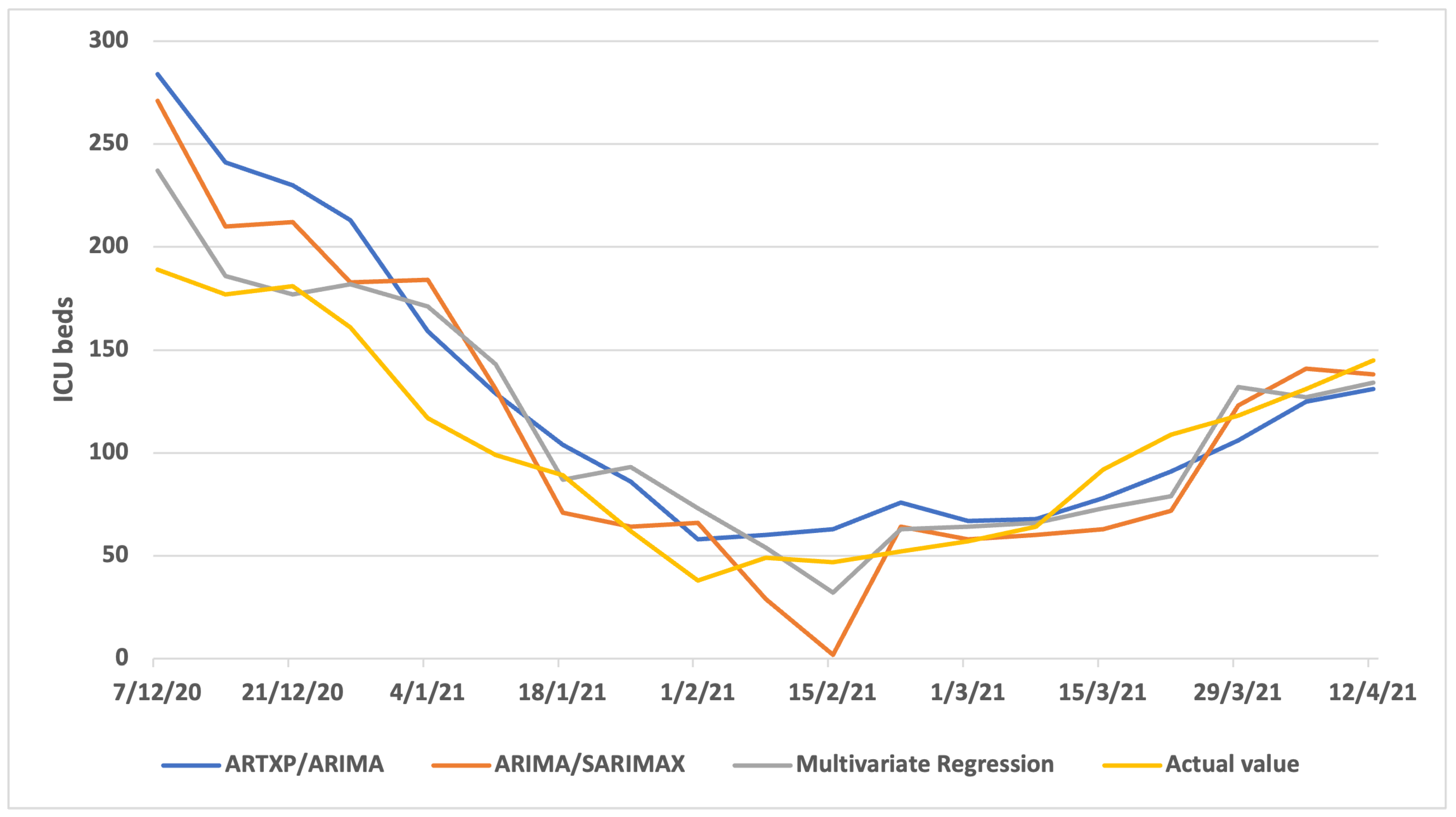
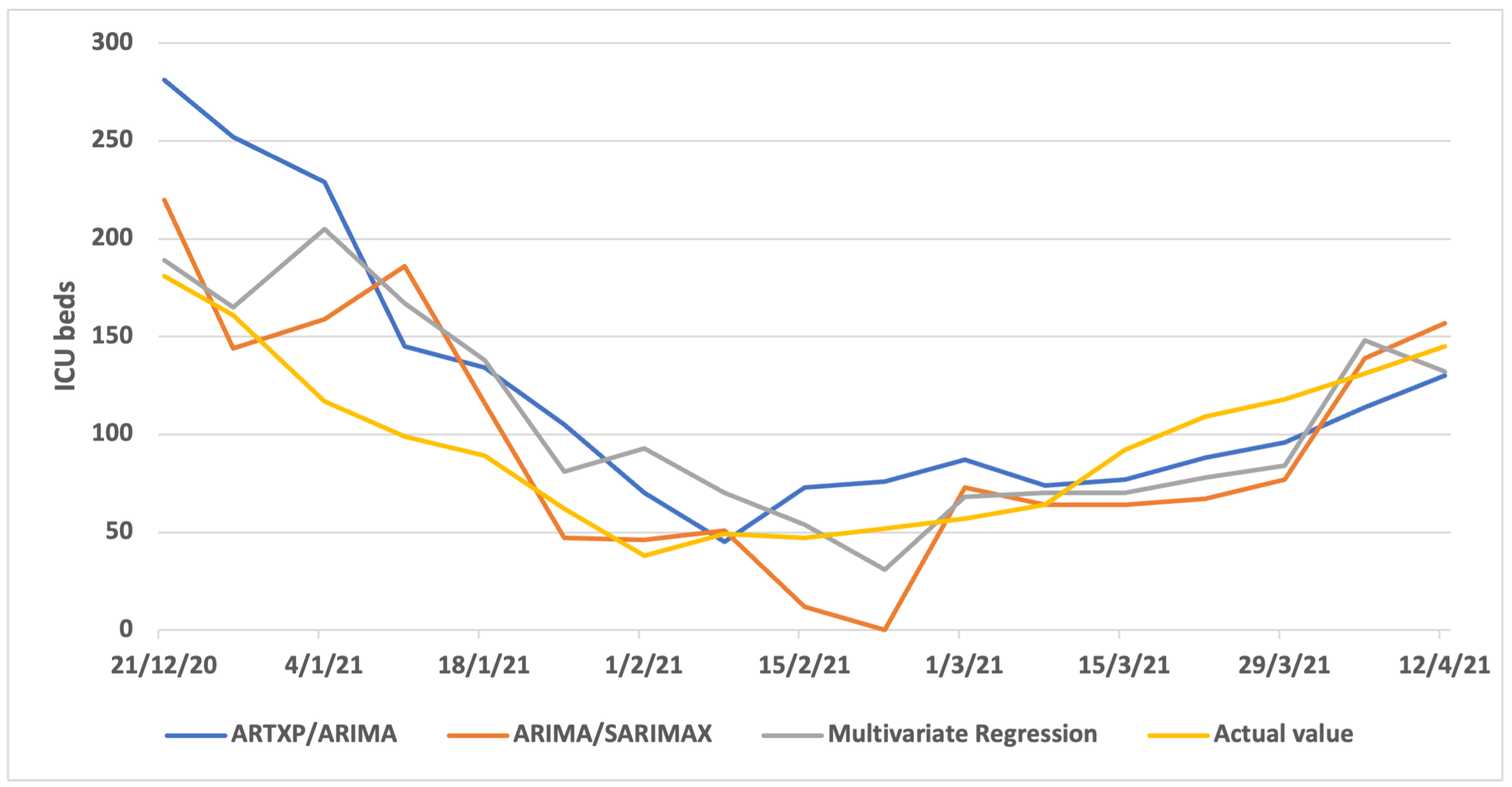
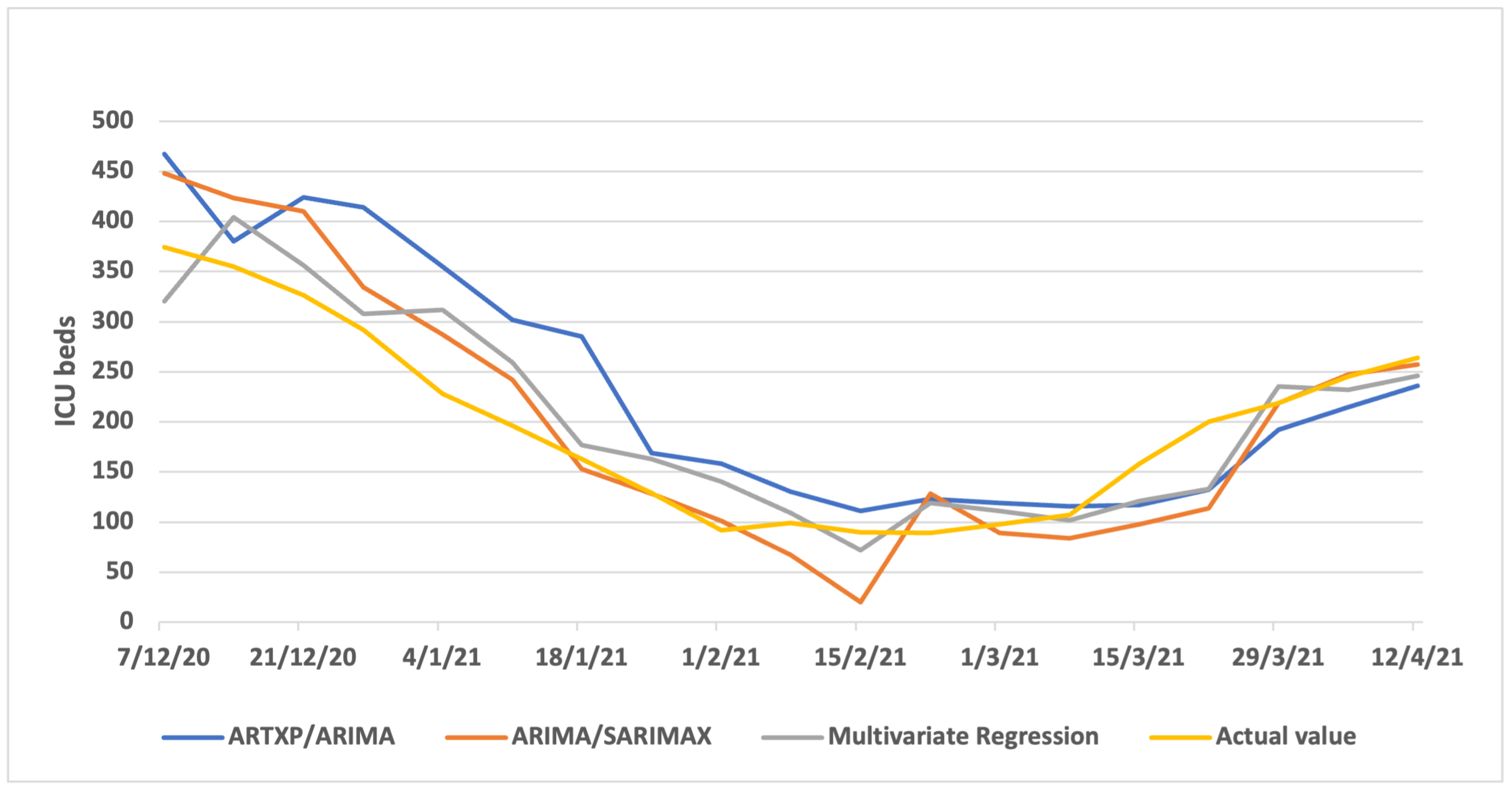
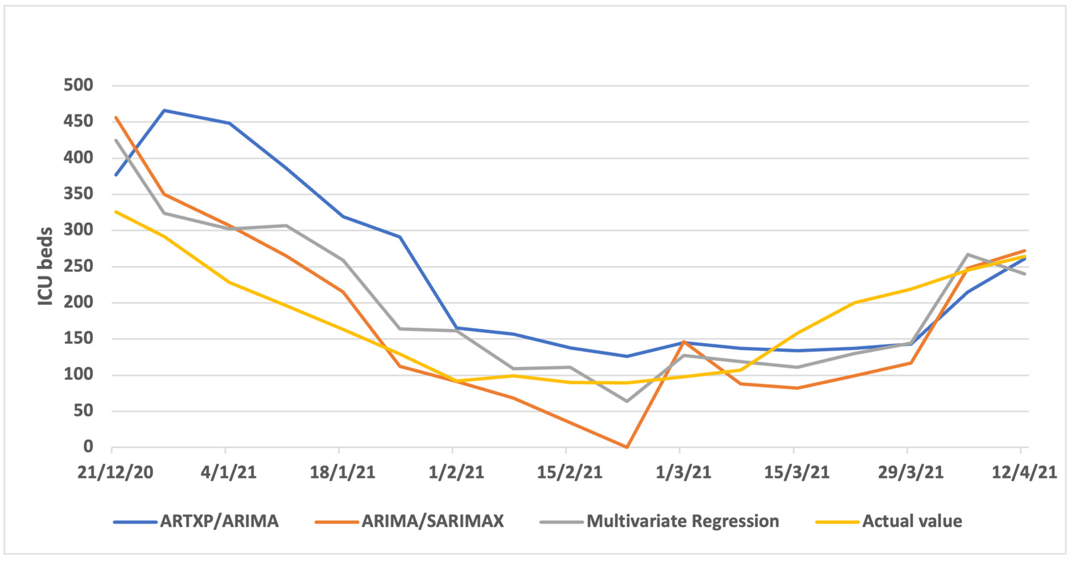
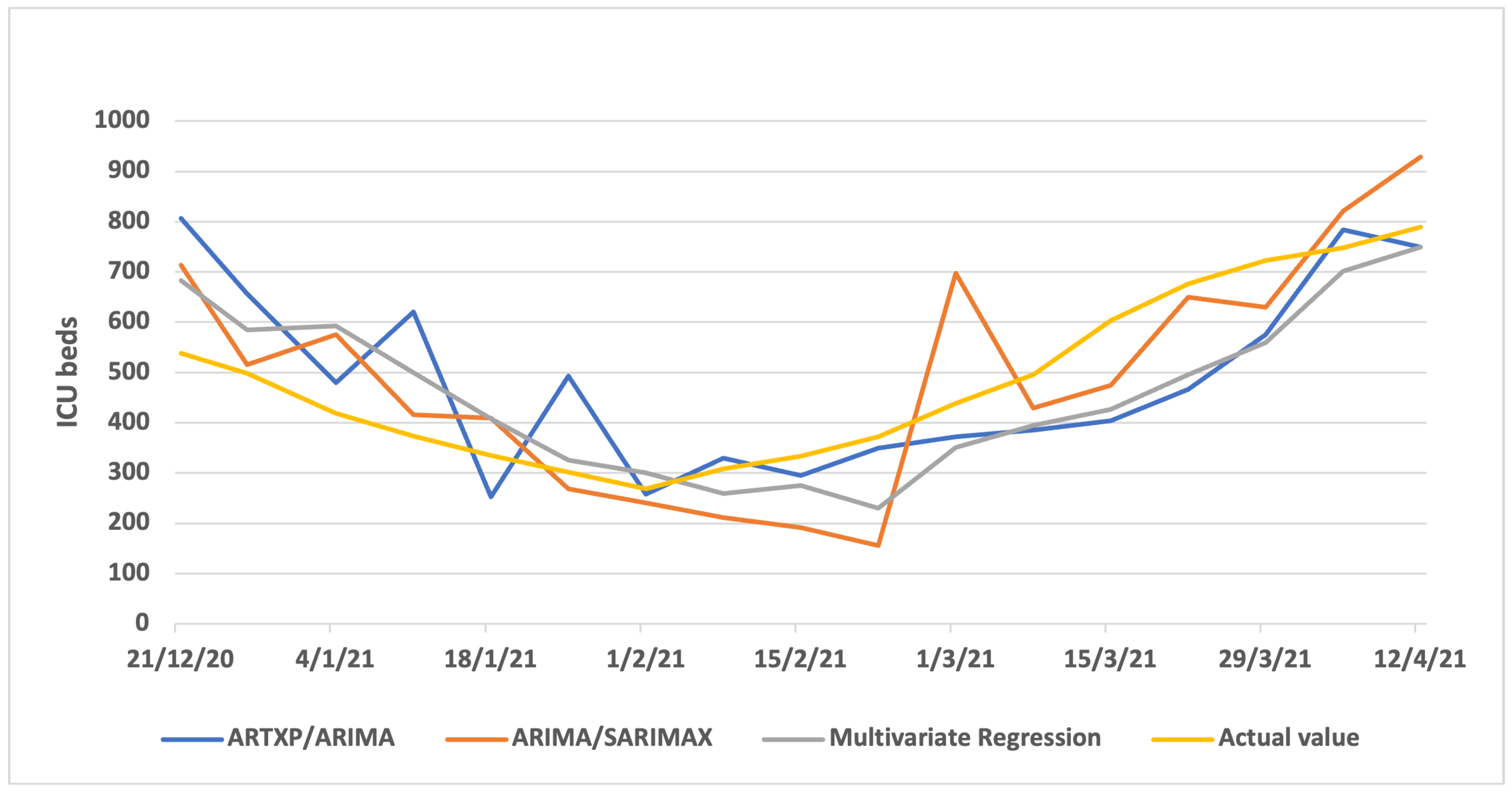
The first region in our report is the prefecture of Thessaloniki. For 1-week ahead predictions, from 23/11 until 22/3 the actual day and 3-day MA of all Models’ Average for MAPE were 11.53% and 10.69%, for RMSE were 16.56 ICUs and 15.14 ICUs, for $R^2$ were 93% and 94%, and for MAE were 12.13 ICUs and 11.04, respectively. Regarding the 2-weeks ahead prediction, from 7/12 until 22/3 the actual day and 3-day MA of all Models’ Average for MAPE were 21.80% and 19.53%, for RMSE were 31.25 ICUs and 28.61 ICUs, for $R^2$ were 85% and 88%, and for MAE were 24.05 ICUs and 22.24 ICUs, respectively. Finally, for the 3-weeks ahead prediction, from 21/12 until 22/3 the actual day and 3-day MA of all Models’ Average for MAPE were 29.80% and 27.95%, for RMSE were 40.27 ICUs and 37.92 ICUs, for $R^2$ were 63% and 68%, and for MAE were 31.33 ICUs and 29.77 ICUs, respectively.

The second region is Northern Greece, including Thessaloniki along with Macedonia, Thrace, Epirus, and Thessaly. For 1-week ahead predictions, from 23/11 until 22/3 the actual day and 3-day MA of all Models’ Average for MAPE were 10.88% and 9.12%, for RMSE were 46.26 ICUs and 43.57 ICUs, for $R^2$ were 95% and 96%, and for MAE were 26.83 ICUs and 23.92 ICUs, respectively. Regarding the 2-weeks ahead prediction, from 7/12 until 22/3 the actual day and 3-day MA of all Models’ Average for MAPE were 20.61% and 17.98%, for RMSE were 52.51 ICUs and 48.33 ICUs, for $R^2$ were 84% and 87%, and for MAE were 42.96 ICUs and 39.38 ICUs, respectively. Finally, for the 3-weeks ahead prediction, from 21/12 until 22/3 the actual day and 3-day MA of all Models’ Average for MAPE were 31.94% and 30.94%, for RMSE were 77.63 ICUs and 74.40 ICUs, for $R^2$ were 63% and 66%, and for MAE were 63.37 ICUs and 60.86 ICUs, respectively.

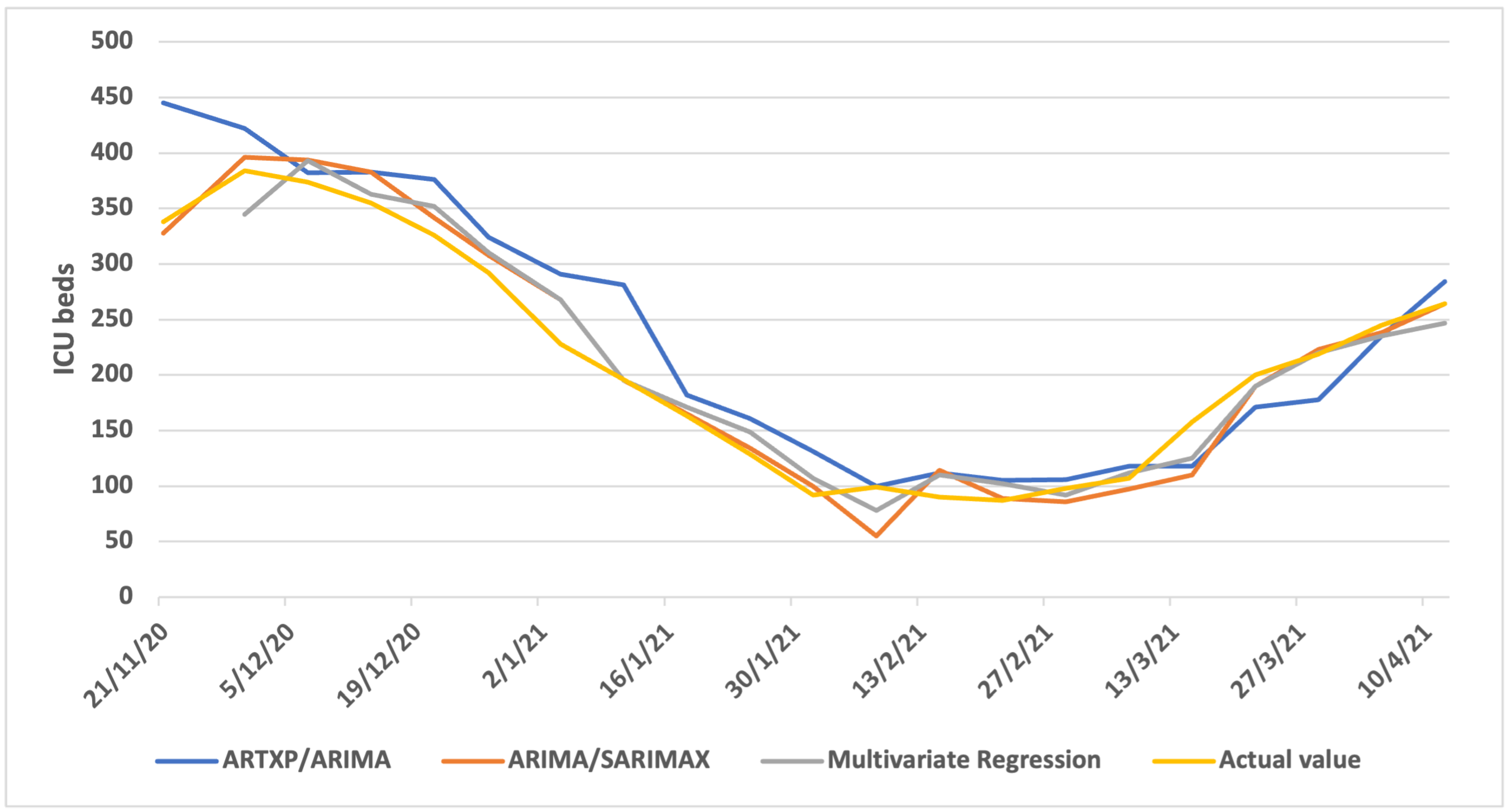
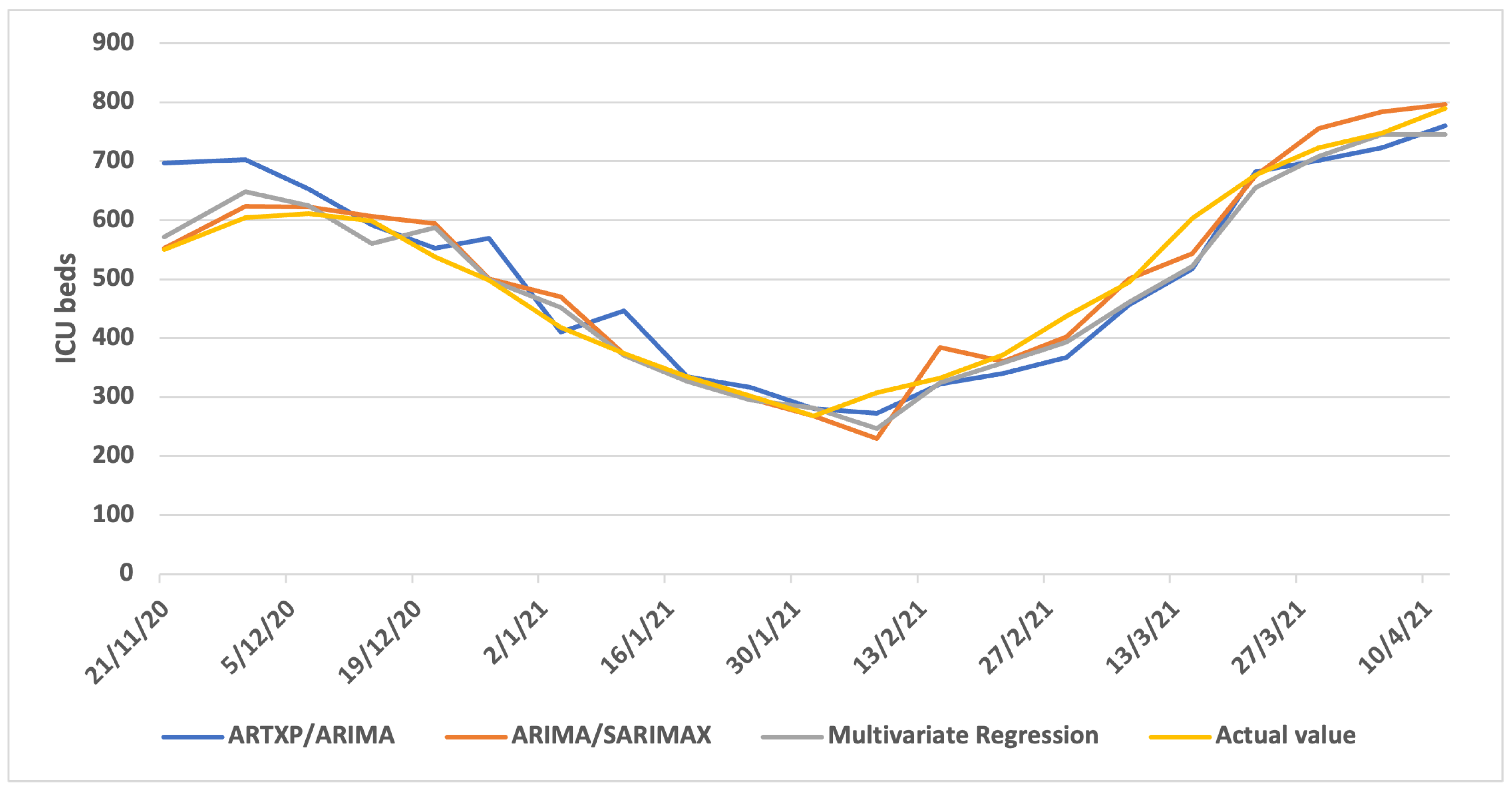
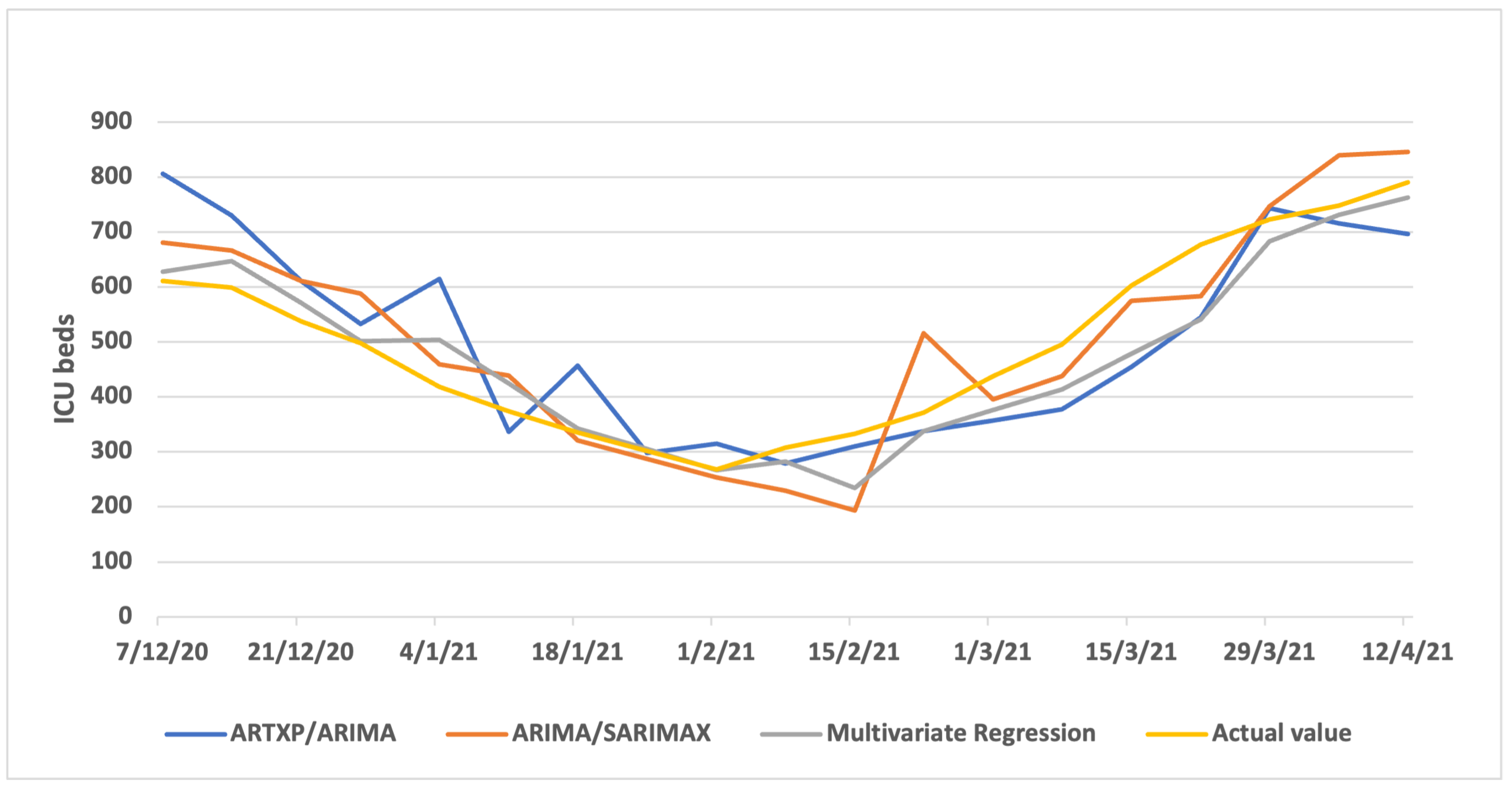
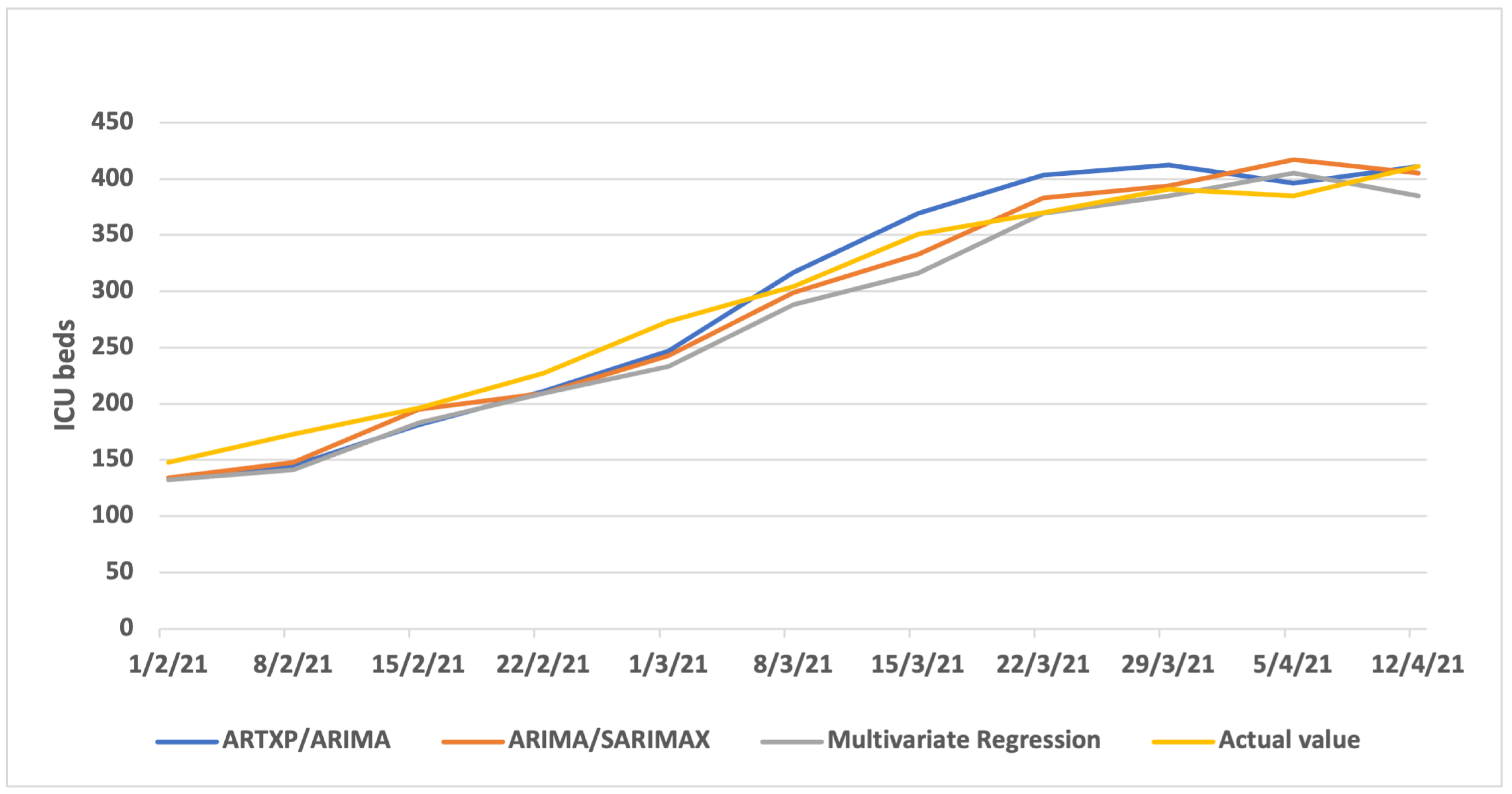
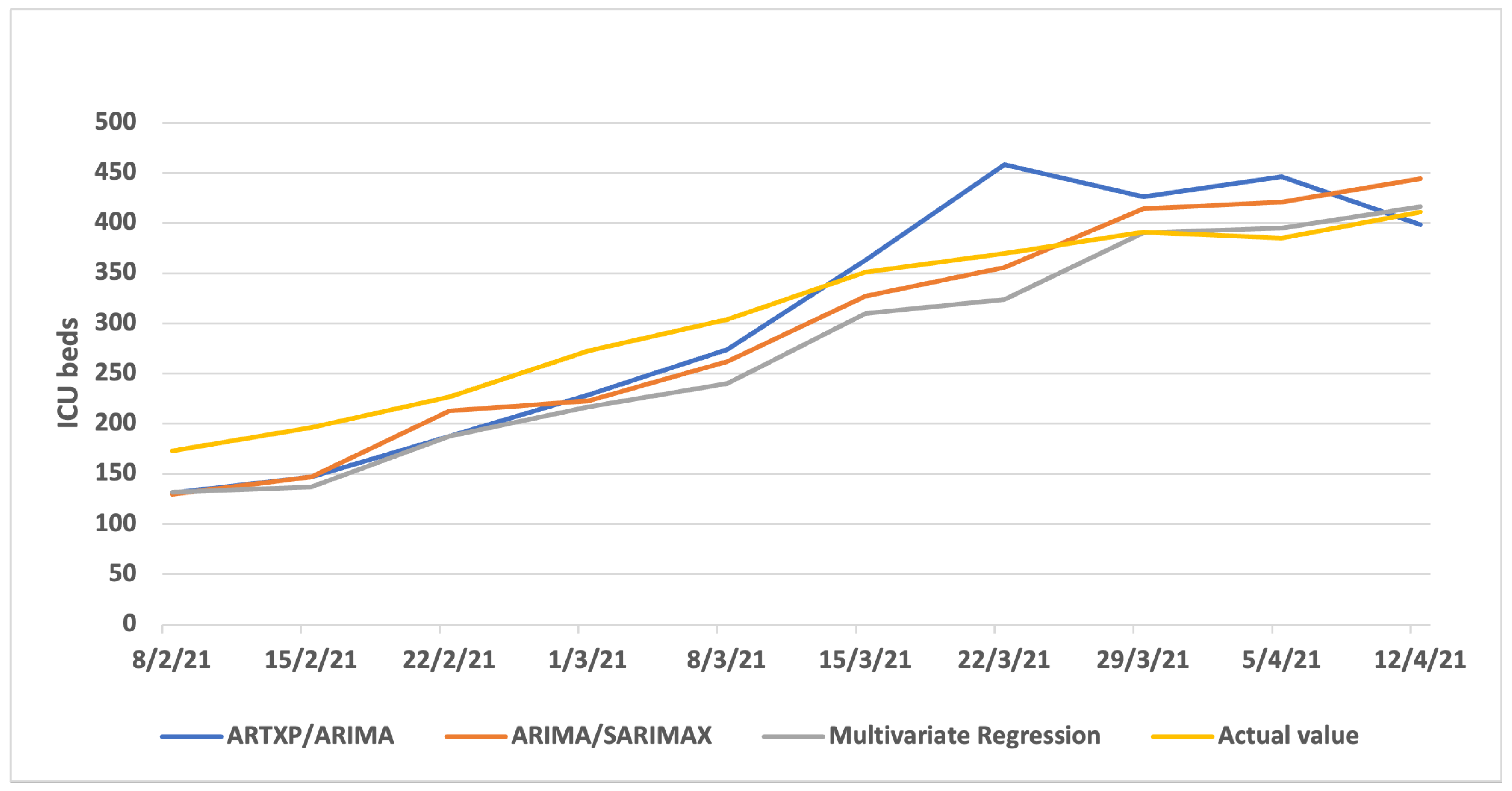
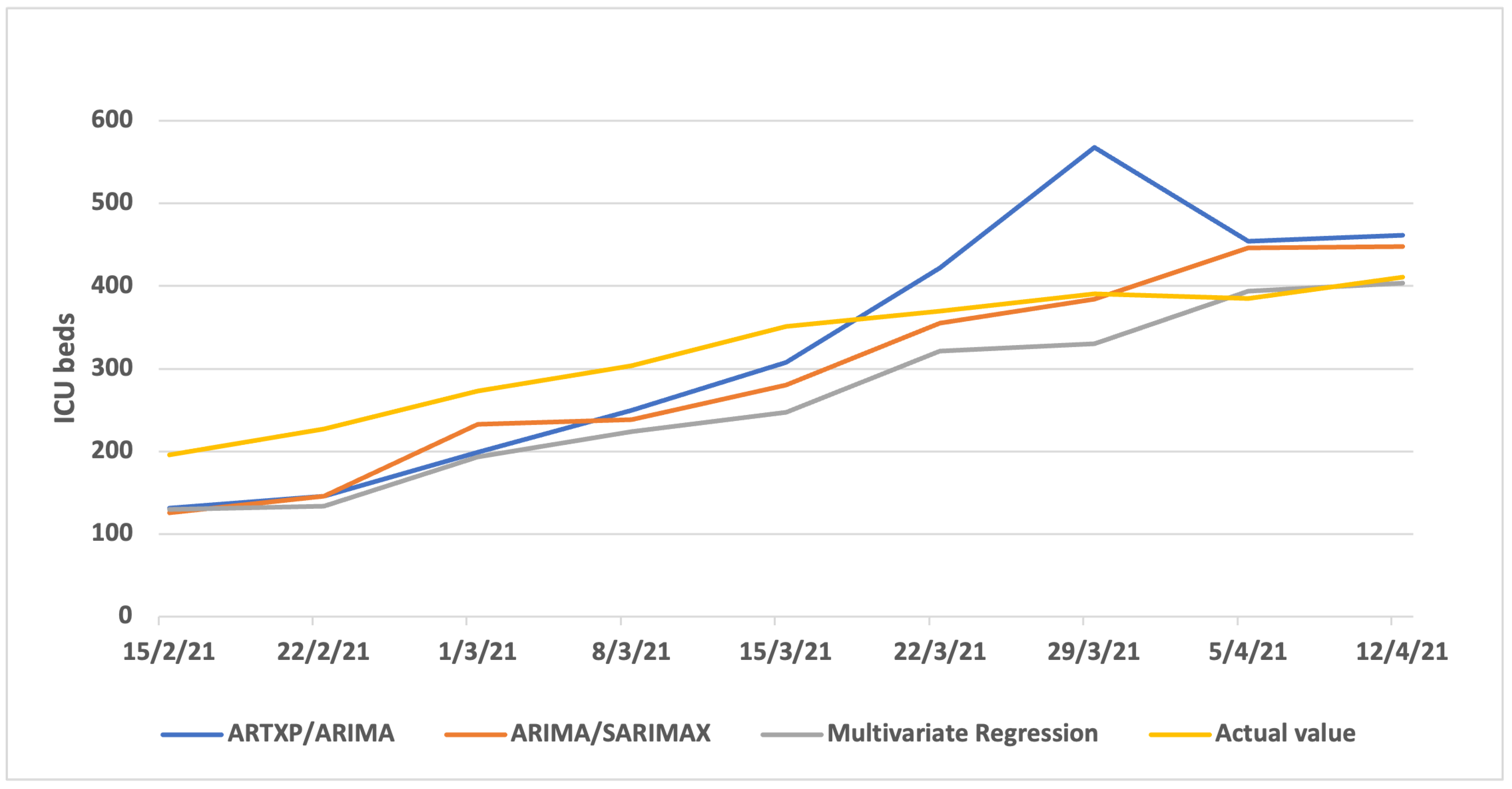
The third region is Greece, nationwide. For 1-week ahead predictions, from 1/2 until 22/3 the actual day and 3-day MA of all Models’ Average for MAPE were 5.45% and 4.73%, for RMSE were 40.44 ICUs and 36.45 ICUs, for $R^2$ were 94% and 95%, and for MAE were 29.89 ICUs and 27.10 ICUs, respectively. Regarding the 2-weeks ahead prediction, from 8/2 until 22/3 the actual day and 3-day MA of all Models’ Average for MAPE were 11.40% and 10.24%, for RMSE were 78.5 ICUs and 73.38 UCUs, for $R^2$ were 81% and 83%, and for MAE were 64.09 ICUs and 58.89 ICUs, respectively. Finally, for the 3-weeks ahead prediction, from 15/2 until 22/3 the actual day and 3-day MA of all Models’ Average for MAPE were 18.81% and 17.86%, for RMSE were 126.05 ICUs and 121.32 ICUs, for $R^2$ were 58% and 61%, and for MAE were 105.61 ICUs and 100.66 ICUs, respectively.

The last region is the prefecture of Attica. For 1-week ahead predictions, from 23 November 2020 until 22 March 2021, the actual day and 3-day MA of all Models’ Average for MAPE were 6.26% and 4.79%, for RMSE were 20.44 ICUs and 17.54 ICUs, for $R^2$ were 98% and 99%, and for MAE were 17.73 ICUs and 15.09 ICUs, respectively. Regarding the 2-weeks ahead prediction, from 7/12 until 22/3 the actual day and 3-day MA of all Models’ Average MAPE were 12.14% and 11.07%, for RMSE were 41.28 ICUs and 38.15 ICUs, for $R^2$ were 95% and 96%, and for MAE were 36.77 ICUs and 33.52 ICUs, respectively. Finally, for the 3-weeks ahead prediction, from 21/12 until 22/3 the actual day and 3-day MA of all Models’ Average MAPE were 18.55% and 17.81%, for RMSE were 69.3 ICUs and 66.22 ICUs, for $R^2$ were 90% and 91%, and for MAE were 61.59 ICUs and 58.29 ICUs, respectively.

In addition, in Table 2, Table 3, Table 4 and Table 5 we highlighted with bold text the best individual value per prediction horizon, model and geographical area. Therefore, for the Thessaloniki area the best values for MAPE are reported by All Models’ Average (1–3 weeks ahead), for RMSE by Multivariate Regression (1–2 weeks ahead) and ARIMA and SARIMAX (3 weeks ahead), for $R^2$ by ARTXP and ARIMA (1–2 weeks ahead) and ARIMA and SARIMAX (1 week and 3 weeks ahead), and for MAE by Multivariate Regression (2–3 weeks ahead) and ARTXP and ARIMA (1 week ahead). For the Northern Greece area, the best values for MAPE are reported by ARIMA and SARIMAX (1 week ahead) and Multivariate Regression (2–3 weeks ahead), for RMSE by ARIMA and SARIMAX (1 week ahead) and Multivariate Regression (2–3 weeks ahead), for $R^2$ by ARIMA and SARIMAX (1–3 weeks ahead), and for MAE by ARIMA and SARIMAX (1 week ahead) and Multivariate Regression (2–3 weeks ahead). For the Greece area, the best values for MAPE are reported by ARIMA and SARIMAX (1 week ahead) and Multivariate Regression (2 weeks ahead) and All Models’ Average (3 weeks ahead), for RMSE by ARIMA and SARIMAX (1 week ahead) and Multivariate Regression (2–3 weeks ahead), for $R^2$ by ARIMA and SARIMAX (1 week and 3 weeks ahead) and Multivariate Regression (2 weeks ahead), and for MAE by ARIMA and SARIMAX (1 week ahead) and Multivariate Regression (2–3 weeks ahead). Finally, for the Attica area, the best values for MAPE are reported by ARIMA and SARIMAX (1 week and 3 weeks ahead) and All Models’ Average (2 weeks ahead), for RMSE by ARIMA and SARIMAX (1–3 weeks ahead), for $R^2$ by ARTXP and ARIMA (1 week ahead) and ARIMA and SARIMAX (2–3 weeks ahead), and for MAE by ARIMA and SARIMAX (1–3 weeks ahead).

Time series models such as ARIMA and ARIMAX, require sufficient amount of historical data to accurately estimate the parameters of the model. During the COVID-19 pandemic, the situation was evolving, and the number of cases could significantly increase or decrease in response to various interventions, such as lockdowns or vaccine rollouts. Regression models typically do not consider the impact of exogenous variables, such as interventions. These interventions can have a significant impact on the number of cases and the demand for ICU beds, and ignoring these factors can lead to inaccurate predictions [28,62,63].

5. Conclusions

The healthcare domain attracts a great amount of research interest, often requiring inter-disciplinary approaches. It involves predictive analytics for prompt forecasting and prevention methods incorporating a mix of concepts from statistics, medicine, computer science etc. [64].

Many countries, including Greece, early on during the COVID-19 epidemic attempted to avoid ICU bed shortage, which could put a strain on intensive care patient management. Accurate forecasting assisted Health authorities to deploy resources and prioritise patient care. ICU bed management during the COVID-19 pandemic emphasises the necessity of accurate forecasting in public health decision making. Health officials were able to respond to patient needs and prevent the healthcare system from becoming overloaded by employing data-driven approaches, saving lives.

This work reports on findings regarding forecasting COVID-19 ICU bed needs during the pandemic. According to the literature, most of the forecasting attempts utilize a mix of SIS and SIR models or incorporate them in their approach [17]. Also, they base their forecasting accuracy in a limited number of observations [11,12,41,43] or report forecasting results for a short timeframe (2 months) [44]. The evaluation of results involves a variety of metrics, such as sensitivity, specificity, accuracy ROC, AUC [11,21,41,43].

In contrast, our approach does not depend on epidemiological models like SIS and SIR; it rather uses a dataset comprising features for a whole country (Greece), it expands the forecasting timeframe to almost 5 months (141 days) and reports findings utilizing four metrics (MAPE, RMSE, $R^2$ and MAE). We argue that these characteristics constitute it an efficient, comprehensive and intelligible novel approach on health related time series forecasting.

We employed various state-of-the-art ML algorithms to address this challenge. The results show that the adopted algorithms performed very well when reporting on their 3-day MA metric values.

For one week ahead predictions using the MAPE metric (Table 2), the best average model was 10.69% for Thessaloniki, 4.79% for Attica, 9.12% for Northern Greece and 4.73% for Greece. For the two weeks ahead predictions the results were expectedly less accurate, the best average model MAPE was 19.53% for Thessaloniki, 11.07% for Attica, 17.98% for Northern Greece and 10.24% for Greece. Even for three weeks ahead forecasting, the results may be useful for healthcare recourse management as the algorithms performed with significantly lower average MAPE, at 27.95% for Thessaloniki, 17.81% for Attica, 30.94% for Northern Greece and 17.86% for Greece. Similar reports apply for the other metrics as shown in Table 3 for RMSE, Table 4 for $R^2$ and Table 5 for MAE.

It should be noted that population-wise Thessaloniki as well as Northern Greece is much smaller than Attica, which hosts nearly half the Greek population, which may partly explain why predictions for Thessaloniki and Northern Greece were substantially less accurate than for Greece or Attica.

Considering the results presented in Table 2, Table 3, Table 4 and Table 5, we conclude that for the short term 1-week ahead prediction, ARIMA and SARIMAX is more accurate for the majority of the investigated regions. For the 2-weeks ahead prediction, Multivariate Regression outperforms the other two models. Finally, for the medium term 3-weeks ahead prediction the Multivariate Regression and ARIMA with SARIMAX show the best results.

5.1. Implications

The pandemic caused enormous pressure on the healthcare systems all over the world. The excessive COVID-19 spread rate forced governments to take specific measures like social distancing, remote working, distance learning, wearing surgery masks or in some cases, wide-ranging lockdowns to mitigate the virus spread. Despite the government measures, there has been a lot of pressure on national health systems, especially on ICUs, which require high standards and scarce resources, such as qualified medical staff.

The exact forecast of ICU requirements can be very useful for the optimal management of finance, resource planning and human resources [65], especially in the short to mid-term where life-saving decisions may take place. Since the human factor is involved, any such attempts should yield high precision results (low statistical error) mitigating disease uncertainty variables and biases. Pressure applies in financial and asset management often relating with materials and medical personnel. For example, ventilators, protection equipment, resource allocation and prioritization. A tool that offers predictive analytics should be able to offer options for relaxing healthcare system pressure, while enhancing the quality of offered services to the patients. Such implementations may constitute sub-components incorporating data mining and ML approaches for smart healthcare support in smart city ecosystems [66].

Governments and policy makers require such produced insights for enforcing policies at local, state or nation-wide level. Timely and efficient public health decision making for optimal resource management offers new capabilities for addressing world-wide event issues (e.g., reducing morbidity and mortality) such as pandemics.

5.2. Future Work

We aim to expand our research on COVID-19 forecasting and optimize our models based on the following directions.

• Regarding the choice of features for forecasting, the utilization of a correlation process that relates virus epidemiological characteristics with metrics may yield even better results [67]. In addition, the impact of temperature, climate and incubation period are important factors which can be used in correlation with demographics or country characteristics [11]. Furthermore, different government mitigation actions (lockdown, social distancing etc.) in terms of time and strictness are also crucial and could be assigned extra weight in the aggregated formula for the predictions [11,68].
• Time series modelling, especially predicting infectious diseases like COVID-19, has heavily exploited LSTM and RNN models. These models predict complex time series trends. They rely on time series length, frequency of observations, number of variables, and training data. These algorithms learn from similar trends, and with more data forecasting accuracy may be improved. Data augmentation and subsampling handle the trade-off between enough data to train the model and too much data that makes it computationally intractable or may cause overfitting. Greece initially had low volume of data. A held-out validation set should rigorously examine the model to avoid overfitting to training data. Thus, enough data against too much data must be carefully considered. Considering the above, future research could also include tests with LSTM and RNN algorithms.
• We also aim to enhance the forecasting capabilities in geographical partitions by utilizing Deep Learning (DL) and ANN. An extra step regarding COVID-19 ICU forecasting would be the use of different and/or combined machine and deep learning algorithms. Since the amount of data is increasing over time and there might be also other parameters that could have a significant impact on COVID-19 infection [9], utilizing DL and ANNs could make a difference. Moreover, other regression algorithms, like RF regressor or XGB regressor could be tested, possibly combined with ANNs like LSTMs [16].
• Finally, according to the reported limitations, identification of time series trend traversal could improve forecasting accuracy. We aim to develop a rule-based methodology that effectively analyses trends in ICU time series and fully adapts them according to changes in trends. Hence, this process would enhance forecasting capabilities by improving the selection of the time series training dataset.