A Hybrid Direct Search and Model-Based Derivative-Free Optimization Method with Dynamic Decision Processing and Application in Solid-Tank Design

Abstract

A derivative-free optimization (DFO) method is an optimization method that does not make use of derivative information in order to find the optimal solution. It is advantageous for solving real-world problems in which the only information available about the objective function is the output for a specific input. In this paper, we develop the framework for a DFO method called the DQL method. It is designed to be a versatile hybrid method capable of performing direct search, quadratic-model search, and line search all in the same method. We develop and test a series of different strategies within this framework. The benchmark results indicate that each of these strategies has distinct advantages and that there is no clear winner in the overall performance among efficiency and robustness. We develop the Smart DQL method by allowing the method to determine the optimal search strategies in various circumstances. The Smart DQL method is applied to a problem of solid-tank design for 3D radiation dosimetry provided by the UBCO (University of British Columbia—Okanagan) 3D Radiation Dosimetry Research Group. Given the limited evaluation budget, the Smart DQL method produces high-quality solutions.

1. Introduction

An optimization problem

$$min\left\{f\left(x\right):x\in \Omega \right\}$$

(1)

is considered a black-box optimization (BBO) problem if the objective function f is provided by a black box. That is, for a given input, the function returns an output, but provides no information on how the output was generated. As such, no higher-order information (gradients, Hessians, etc.) are available. Developing methods to solve BBO problems is a highly valued field of research, as the methods are used in a wide range of applications [1,2,3,4,5,6,7,8] (amongst many more).

In many BBO problems, heuristic techniques are used [1,2,3]. In this paper, we focus on provably convergent algorithms. The study of provably convergent algorithms that do not explicitly use high-order information in their execution is often referred to as derivative-free optimization (DFO). We refer readers to [9,10] for a general overview of DFO and to [11,12] for recent surveys of applications of DFO.

DFO is often separated into two disjoint strategies: direct search methods and model-based methods [10]. Direct search methods involve looking for evaluation candidate(s) directly in the search domain [9,10]. Conversely, model-based methods involve building a surrogate model from the evaluated points to find the next evaluation candidate [9,10]. As DFO research has advanced, researchers have proposed that these two strategies should be merged to create hybrid algorithms that applied both techniques [9,10,13,14,15]. However, very few algorithms have been published that hybridize theses two methods.

In this research, we seek to develop a framework that allows for direct search and model-based methods to be united into a single algorithm. We further seek to develop dynamic approaches to select and adjust how the direct search and model-based methods are used. In doing so, we aim to apply both a mathematical analysis that guarantees convergence (under reasonable assumptions) and numerical testing to determine techniques that work well in practice.

1.1. Overview of DQL and Smart DQL Method

Some efforts have been made to hybridize direct search and model-based methods. For example, the SID-PSM method involves combining a search step of minimizing the approximated quadratic model over a trust region with the direct search [13,14]. The rqlif method, which we discuss next, provides a more versatile approach [15].

To understand the rqlif method, we note that there are two common ways to find the next evaluation candidate during a model-based method [10]. First, methods can find the candidate at the minima of the surrogate model within some trust region or constraints. These are referred to as model-based trust-region (MBTR) methods. Second, methods can use the model to predict the descent direction and perform a line-search on the direction. These are referred to as model-based descent (MBD) methods.

At each iteration, the rqlif method searches for an improvement using three distinct strategies without relying on gradient or higher-order derivative information. These steps are referred to as the direct step, quadratic step, and linear step. These three steps correspond to three distinct search strategies from the direct search method, MBTR methods, and MBD methods.

Inspired by the structure of the rqlif method, we propose the DQL method framework. The purpose of this framework is to allow a flexible hybrid method that permits a direct search, quadratic-model search, and line-search all in the same method. Our objective is to design a framework that allows the development of a variety of search strategies and to determine the strategies that perform best. The DQL method is a local method for solving unconstrained BBO problems. We ensure its local convergence by implementing a two-stage procedure. The first stage focuses on finding an improvement in an efficient manner. It accepts an improvement whenever the candidate yields a better solution. We call this stage the exploration stage. The second stage focuses on the convergence to a local optimum; we call this stage the convergence stage.

In Section 2, we introduce the DQL method’s framework and the search strategies. In Section 3, we conduct the convergence analysis. Provided that the objective function has a compact level set $L\left(x_0\right)$ and the gradient of the objective function is Lipschitz continuous in an open set containing $L\left(x_0\right)$, the convergence analysis indicates that there exists a convergent subsequence of iterations with a gradient of zero at its limit. This demonstrates that when the evaluation budget is large enough, the method will converge to a stationary point.

Using the framework of the DQL method, we obtain a series of combinations of quadratic and linear step strategies. In order to select the best combination among them, in Section 3, we perform a numerical benchmark across all the possible combinations. The quadratic step strategies are capable of improve the overall performance of the method. However, the linear steps show a mixed performance and there is no clear winner on efficiency or robustness. This inspires the idea that by employing an appropriate strategy in certain circumstances, we may be able to achieve an overall improvement in performance.

This idea of allowing the method to make decisions on search strategies in various circumstances leads to the Smart DQL method, which we discuss in Section 4. By analyzing the search results from various strategies, we develop decision processes that select the appropriate strategies for the search steps during the optimization. This allows the method to dynamically decide the appropriate strategies for the given information. In Section 4, we perform numerical tests on the Smart DQL method and discover that the Smart DQL method outperforms the DQL methods in terms of both robustness and performance.

In Section 5, we apply the Smart DQL method to the problem of design of solid tanks for optical computed tomography scanning of 3D radiation dosimeters described in [16]. The original paper employs a grid-search technique combined with a manual refinement to solve the problem. This process involves considerable human interaction. Conversely, we find that the Smart DQL method is capable of producing a high-quality solution without human interaction.

1.2. Definitions

Throughout this paper, we assume $f:{\mathbb{R}}^n\to \mathbb{R}$. Let $x_{\mathrm{best}}^k$ denote the best solution found by the method at iteration k and $f_{\mathrm{best}}^k$ denote the corresponding function value.

We present the definitions that are used to approximate gradient and Hessian by the DQL method as follows. We begin with the Moore–Penrose pseudoinverse.

Definition 1  

(Moore–Penrose pseudoinverse). Let $A\in {\mathbb{R}}^{n\times m}$. The  Moore–Penrose pseudoinverse of A, denoted by $A^{†}$, is the unique matrix in ${\mathbb{R}}^{m\times n}$ that satisfies the following four equations:

$$A{A}^{†}A=A,$$

(2)

$$A^{†}A{A}^{†}=A,$$

(3)

$${\left(A{A}^{†}\right)}^{\top }=A{A}^{†},$$

(4)

$${\left(A^{†}A\right)}^{\top }=A^{†}A.$$

(5)

The generalized centred simplex gradient and generalized simplex Hessian are studied in [17,18], respectively.

Definition 2  

(Generalized centred simplex gradient [17]). Let $f:{\mathbb{R}}^n\to \mathbb{R}$, $x_0\in {\mathbb{R}}^n$ be the point of interest, and $D=\left[\begin{array}{cccc}{d}^1& d^2& \cdots & d^k\end{array}\right]\in {\mathbb{R}}^{n\times k}$. The generalized centred simplex gradient of f at $x_0$ over D is denoted by ${\nabla }_{c}f(x_0;D)$ and defined by,

$${\nabla }_{c}f(x_0;D)={\left(D^{\top }\right)}^{†}{\delta }_f^c(x_0;D)\in {\mathbb{R}}^n,$$

(6)

where

$${\delta }_f^c(x_0;D)=\frac{1}{2}{\left[\begin{array}{ccc}f(x_0+d^1)-f(x_0-d^1),& \cdots ,& f(x_0+d^k)-f(x_0-d^k)\end{array}\right]}^{\top }.$$

(7)

Definition 3  

(Generalized simplex Hessian). Let $f:{\mathbb{R}}^n\to \mathbb{R}$ and $x_0$ be the point of interest. Let $S=\left[\begin{array}{cccc}{s}^1& s^2& \cdots & s^m\end{array}\right]\in {\mathbb{R}}^{n\times m}$ and $\{D^i:D^i\in {\mathbb{R}}^{n\times k},i=0,1,2,\cdots ,m\}$ be the set of direction matrices used to approximate the gradients at $x_0, x_0+s^1,\cdots ,x_0+s^m$, respectively. The generalized simplex Hessian of f at $x_0$ over S and $\left\{D^i\right\}$ is denoted by ${\nabla }_s^{2}f(x_0;S,\left\{D^i\right\})$ and defined by

$${\nabla }_s^{2}f(x_0;S,\left\{D^i\right\})={\left(S^{\top }\right)}^{†}{\delta }_{{\nabla }_{c}f}(x_0;S,\left\{D^i\right\}),$$

(8)

where

$${\delta }_{{\nabla }_{c}f}(x_0;S,\left\{D^i\right\})=\left[\begin{array}{c}{({\nabla }_{c}f(x_0+s^1;D^1)-{\nabla }_{c}f(x_0;D^0))}^{\top }\\ {({\nabla }_{c}f(x_0+s^2;D^2)-{\nabla }_{c}f(x_0;D^0))}^{\top }\\ ⋮\\ {({\nabla }_{c}f(x_0+s^m;D^m)-{\nabla }_{c}f(x_0;D^0))}^{\top }\end{array}\right]\in {\mathbb{R}}^{m\times n}.$$

(9)

In Section 3, in order to prove convergence of our method, we make use of the cosine measure as defined in [9].

Definition 4  

(Cosine measure). Let $D=\left[\begin{array}{cc}{d}^1& d^2,\cdots ,d^m\end{array}\right]\in {\mathbb{R}}^{n\times m}$ form a positive basis. We say D forms a positive basis if $\{x:x={\sum }_{i=1}^m\lambda d^i,\lambda \ge 0\}=R^n$ but no proper subset of D has the same property. The cosine measure of D is defined by,

$$cm\left(D\right)=\underset{\omega \in {\mathbb{R}}^n}{min}\left\{\underset{d\in D}{max}\left\{\frac{{\omega }^{\top }d}{∥\omega ∥∥d∥}\right\}:∥\omega ∥=1\right\}.$$

(10)

2. DQL Method

In this section, we introduce the framework of the DQL method. At each iteration, the method starts from an initial search point $x_0^k$ and a search step length ${\delta }^k$. Note that at the first iteration, the initial search point and the search step length are given by the inputs $x_0$ and ${\delta }_0$, so $x_0^1=x_0$ and ${\delta }^1={\delta }_0$. The initial search point and the search step length are used to initiate three distinct search steps: the direct step, the quadratic step, and the linear step. A variable $x_{\mathrm{best}}^k$ is used to track the current best solution at iteration k. If an improvement is found in the search step length at iteration k, the method updates $x_{\mathrm{best}}^k$. Three Boolean values are used to track the results from each search step: Direct_Flag, Quadratic_Flag, and Linear_Flag. If a search step succeeds at finding an improvement, it sets the corresponding Flag to true; otherwise, the corresponding Flag is set to false. These search steps are then followed by the update step. In the update step, the search step length is updated according to the search results and the method uses the current best solution as the starting search point of the next iteration.

As mentioned, the DQL method utilizes two different stages: the exploration stage and the convergence stage. In the exploration stage, the method enables all the search steps, and it accepts the improvement whenever the evaluation candidate yields a lower value than the current best solution. If the iteration counter k reaches the given max_search, then the method proceeds with the convergence stage, the method disables the quadratic and the linear step and the solution acceptance implements a sufficient decrease rule.

This framework allows various search strategies to be implemented. We provide some basic strategies for performing the search steps. The analysis of the convergence and the performance of these search steps are discussed in the next section.

2.1. Solution Acceptance Rule

In the DQL method, each search step returns a set of candidate(s). Then, these candidate(s) are evaluated and compared to the current best solution $x_{\mathrm{best}}^k$. If the best candidate is accepted by the solution acceptance rule, then $x_{\mathrm{best}}^k$ is updated. There are two solution acceptance rules that are used in the DQL method. The first rule is used in the exploration stage and updates $x_{\mathrm{best}}^k$ whenever an improvement is found. The second rule is used in the convergence stage and updates $x_{\mathrm{best}}^k$ only when the candidate makes sufficient decrease. Specifically, in the convergence stage of the DQL method, a candidate $x_{\mathrm{current}}\in$ Candidate_Set is accepted as $x_{\mathrm{best}}^k$ only if

$$f\left(x_{\mathrm{current}}\right)<f\left(x_{\mathrm{best}}^k\right)-{\left({\delta }^k\right)}^2,$$

(11)

where ${\delta }^k$ is the current search step length. We show that this sufficient decrease rule is crucial for the convergence of the DQL method in the next section. The algorithm of the solution acceptance is denoted as

Improvement_Check (Candidate_Set, $x_{\mathrm{BEST}}^k$, ${\delta }^k$)

and is shown in Algorithm 1.

Algorithm 1 Improvement_Check (Candidate_Set, $x_{\mathrm{BEST}}^k$, ${\delta }^k$)

1: Evaluate Candidate_Set   2: $x_{\mathrm{current}}\leftarrow arg\; min\{\mathrm{function}\mathrm{evaluations}\mathrm{of}$Candidate _ Set}   3: if$k\le$MAX_SEARCH  then   4:     if $f\left(x_{\mathrm{current}}\right)<f\left(x_{\mathrm{best}}^k\right)$ then   5:         $x_{\mathrm{best}}^k\leftarrow x_{\mathrm{current}}$   6:     end if   7: else   8:     if $f\left(x_{\mathrm{current}}\right)<f\left(x_{\mathrm{best}}^k\right)-{\left({\delta }^k\right)}^2$ then   9:         $x_{\mathrm{best}}^k\leftarrow x_{\mathrm{current}}$ 10:     end if 11: end if

2.2. Direct Step

2.2.1. Framework of the Direct Step

In the direct step, the method searches from the starting search point $x_0^k$ in the positive and negative coordinate directions or a rotation thereof. We denote the set of search directions at iteration k as ${\overline{D}}^k$. The positive and negative coordinate directions can be written as the columns of an $n\times 2n$ matrix $\left[\begin{array}{cc}{I}_n& -I_n\end{array}\right]$. The method applies an $n\times n$ rotation matrix $D^k=\left[\begin{array}{cccc}{d}_1^k& d_2^k& \cdots & d_n^k\end{array}\right]\in {\mathbb{R}}^{n\times n}$, so $D^k$ can be written as $\left[\begin{array}{cc}{D}^k& -D^k\end{array}\right]$.

We first need to determine how we want to rotate the search directions. We have two possible situations. First, if the method predicts a direction for which improvement is likely to be found, then we call this direction a desired direction. Notice that, since we search on both positive direction and negative direction, we also search the direction where an improvement is unlikely to be found. Conversely, if the method predicts a direction that is highly unlikely to provide improvement, then we call the corresponding direction an undesired direction. Denoting the predicted direction by $r^k$, we have the following 2 possibilities.

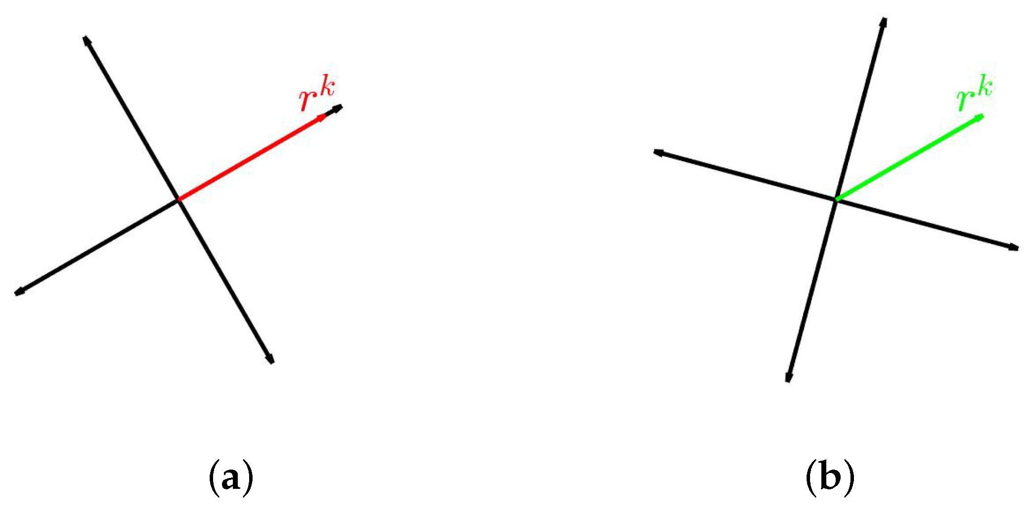
• If $r^k$ is a desired direction, then we construct $D^k$ such that it rotates one of the search directions to align with $r^k$.
• If $r^k$ is an undesired direction, then we construct $D^k$ such that it rotates the vector $\left[\begin{array}{ccc}1& \cdots & 1\end{array}\right]$ to align with $r^k$. In this way, the coordinate directions are rotated to point away from $r^k$ as much as possible.

Figure 1 shows how the method rotates the search direction matrix $D^k$ towards a desired direction or away from an undesired direction for an ${\mathbb{R}}^2$ problem.

Figure 1. An example of rotating search direction $D^k$ (black) for (a) a desired direction (red) and (b) an undesired direction (green). (a) Align ${\overline{D}}^k$ towards the desired direction $r^k$. (b) Align ${\overline{D}}^k$ away from the undesired direction $r^k$.

For an n-dimensional rotation $(n>3)$, the rotation is described as rotating by an angle of $\alpha$ on an $n-1$ dimension hyperplane that is spanned by a pair of orthogonal unit vectors u and $v\in {\mathbb{R}}^n$. According to Masson, such a rotation matrix D can be defined as follows [19],

$$L(\alpha ,u,v)=I_n+(v{u}^{\top }-u{v}^{\top })sin\alpha +(u{u}^{\top }+v{v}^{\top })(cos\alpha -1).$$

(12)

For a desired direction $r^k$, the rotation matrix $D^k$ can be found by rotating the coordinate directions on the hyperplane spanned by one coordinate direction, e.g., $e_1$, and $r^k$ by the angle between $e_1$ and $r^k$. Notice that if $e_1$ and $r^k$ are linearly dependent, then $r^k$ lies on the coordinate direction $e_1$, so $D^k$ is the identity matrix. In conclusion, if $r^k$ is a desired direction, the search directions $D^k$ is calculated as follows,

$$D^k=L(arccos\left({r^k}^{\top }{e}_1\right),r^k,e_1).$$

(13)

For an undesired direction $r^k$, the method needs to keep the search directions as far from $r^k$ as possible. In order to do so, it first constructs a normalized one-vector $\widehat{\mathbf{1}}$, which is calculated as follows,

$$\widehat{\mathbf{1}}=\frac{{\Sigma }_{i=1}^n{e}_i}{∥{\Sigma }_{i=1}^n{e}_i∥}=\frac{{\Sigma }_{i=1}^n{e}_i}{\sqrt{n}}.$$

(14)

Then, the method aligns $\widehat{\mathbf{1}}$ with the undesired direction $r^k$. The rotation matrix $D^k$ for an undesired direction $r^k$ is calculated as follows,

$$D^k=L(arccos\left({r^k}^{\top }\widehat{\mathbf{1}}\right),r^k,\widehat{\mathbf{1}}).$$

(15)

After the search directions $D^k$ are built, the search candidates from the direct step at iteration k can be determined as

$${\mathbb{D}}^k=\{x_0^k+{\delta }^k{d}^k:d^k\in {\overline{D}}^k\}.$$

(16)

We then check if any of the candidates yield improvement by

Improvement_Check(${\mathbb{D}}^k$, $x_{\mathrm{best}}^k$, ${\delta }^k$).

If an improvement is found, then the Direct_Flag is set to be true. Otherwise, the Direct_Flag is set to be false.

The pseudocode of the direct step in the DQL method is shown in Algorithm 2. The direct step is always initiated at every iteration, and it produces $|{\mathbb{D}}^k|=2n$ candidates, so it requires $2n$ function evaluations to perform. Since these candidates are independent from each other, the function evaluations proceed in parallel. Although this step is computationally expensive, it is necessary to prove convergence of our method as shown in Theorem 4. The freedom of choosing the rotation direction is essential to the development of the Smart DQL method. This allows us to develop a variety of rotation strategies that are discussed in the next section.

Algorithm 2Direct_Step ($x_0^k$, ${\delta }^k$)

1: Determine the rotation direction $r^k\in {\mathbb{R}}^n$ 2: if$r^k$ is a desired direction then 3:     Align $D^k$ towards $r^k$ 4: else 5:     Align $D^k$ away from $r^k$ 6: end if 7: The direct search candidates ${\mathbb{D}}^k=\{x_0^k+{\delta }^k{d}^k:d^k\in {\overline{D}}^k\}$ 8: improvement_check(${\mathbb{D}}^k$, $x_0^k$, ${\delta }^k$) 9: Update Direct_Flag accordingly

Direct Step Strategy

The first direct step strategy is inspired by the direct step in the rqlif method [15]. The rotation directions alternate between two options:

• A coordinate direction being the desired direction;
• A random direction being the desired direction.

At odd iterations, the method searches on the positive and negative coordinate directions. At even iterations, the method searches on the random rotations of the coordinate directions. We denote this strategy as direct step strategy 1. In Section 4, when developing the Smart DQL method, we introduce new rotation strategies.

2.3. Quadratic Step

2.3.1. Framework of Quadratic Step

If the direct step fails to find an improvement, then the method proceeds to the quadratic step. Note that after a failed direct step, the best point remains at $x_0^k$. In the quadratic step, the method first selects the points that have been previously evaluated within some radius $q^k\ge \beta {\delta }^k$ of the point of centre $x_0^k$ for some $\beta \ge 1$. These points are used to construct a quadratic model of the objective function. The radius condition $q^k\ge \beta {\delta }^k$ ensures that all the points from the direct search are taken into account. The method extracts the quadratic information from these calculated points using a least-squares quadratic model or Hessian approximation. The pseudocode of the quadratic step is shown in Algorithm 3. Note that in the third line of Algorithm 3, the methods of extracting and utilizing the quadratic information varies for different strategies. The idea of the quadratic step is to use these previously evaluated points $\left\{x_i\right\}$ to predict a candidate by using quadratic approximations.

Algorithm 3 Quadratic_Step ($x_0^k$, $\beta$, ${\delta }^k$, $\left\{x_i\right\}$)

1: $q^k\leftarrow \beta {\delta }^k$ 2: Determine the set of evaluated points within the trust region $Q^k=\{x_i:∥x_i-x_0^k∥\le q^k\}$ 3: Determine the quadratic search candidates ${\mathbb{Q}}^k$ using the quadratic information from $Q^k$ 4: improvement_check (${\mathbb{Q}}^k$, $x_0^k$, ${\delta }^k$) 5: Update Quadratic_Flag accordingly

Quadratic Step Strategies

Our first option for the quadratic step begins by constructing a least-squares quadratic model. We use the quadprog and trust functions from Matlab [20] to find the least-squares quadratic model and its optimum within the trust region. We label this quadratic step strategy as quadratic step strategy 1.

Our second option for the quadratic step is to take one iteration of an approximated Newton’s method. Approximation techniques are introduced to obtain the required gradient and Hessian. Notice that at the end of the direct step, the centred simplex gradient approximation is performed, so we take

$$\nabla f\left(x_0^k\right)\approx {\nabla }_{c}f(x_0^k;{\delta }^k{D}^k).$$

(17)

To approximate the Hessian at $x_0^k$, we need all the points within radius $q^k$ that have a gradient approximation. Since the gradient approximations are performed in previous unsuccessful direct steps, we can reuse those approximation. First, the points that have gradient approximation and are within the radius $q^k$ are determined. We denote these by $x_h^j$$(j=1,2,\cdots ,m)$. The corresponding search directions and search step lengths are denoted by $D_h^j$ and ${\delta }_h^j$$(j=1,2,\cdots ,m)$. We take $D_h^0$ and ${\delta }_h^0$ as the search direction and search step length in the direct step of the current iterate. We obtain

$$S=\left[\begin{array}{cccc}{x}_h^1-x_0^k& x_h^1-x_0^k& \cdots & x_h^m-x_0^k\end{array}\right].$$

(18)

The Hessian at $x_0^k$ can be approximated as,

$${\nabla }^{2}f\left(x_0^k\right)\approx {\nabla }_s^{2}f(x_0^k;S,\left\{{\delta }_h^j{D}_h^j\right\})={\left(S^{\top }\right)}^{†}{\delta }_{{\nabla }_{c}f}(x_0^k;S,\left\{{\delta }_h^j{D}_h^j\right\}),$$

(19)

where ${\delta }_{{\nabla }_{c}f}(x_0^k;S,\left\{{\delta }_h^j{D}_h^j\right\})$ is defined in Definition 3.

If the approximated Hessian is positive definite, then the search candidate is determined via

$$x_Q=x_0^k-{\left({\nabla }_s^{2}f(x_0^k;S,\left\{{\delta }_h^j{D}_h^j\right\})\right)}^{-1}{\nabla }_{c}f(x_0^k;{\delta }^k{D}^k).$$

(20)

If the approximate Hessian is not positive definite, we can perform a trust-region search by building a quadratic model with the approximate gradient and Hessian at $x_0^k$.

We label this quadratic step strategy as quadratic step strategy 2.

Discussion on Quadratic Step Strategies

Both quadratic step strategies try to build a quadratic model and extract the optima from the quadratic model. However, there are some major differences between the two strategies.

• The points chosen to construct the model are different. In the quadratic step strategy 1, any evaluated points that are within the trust region are chosen. In the quadratic step strategy 2, the chosen points have an additional requirement that they should also have a gradient approximation.
• In the quadratic step strategy 1, $x_Q$ lies within the trust region. In the quadratic step strategy 2, if the approximated Hessian is positive definite, then $x_Q$ may lie outside of the trust region.

We demonstrate in the numerical benchmarking that these differences lead to distinct behaviours and performances.

2.4. Linear Step

2.4.1. Framework of Linear Step

If the quadratic step fails to find an improvement, then the method performs the linear step. The idea of the linear step is to find evaluation candidate(s) in a desired direction $d\in {\mathbb{R}}^n$ at some step length(s) ${\alpha }^j\in {\mathbb{R}}^n$. The search candidates can be obtained as

$$x_l^j=x_0^k+{\alpha }^{j}d,$$

(21)

and we denote the set of all candidates as ${\mathbb{L}}^k$. The idea of the linear step is to perform a quick search in the direction that is likely to be a descent direction. The pseudocode of the linear step in the DQL method is shown in Algorithm 4. Note that in order to perform Line 2 of Algorithm 4, there are two components we need to determine: the desired direction and the step length(s). We discuss this in the next section.

Algorithm 4 Linear_Step ($x_0^k$, ${\delta }^k$)

1: Determine the search direction $d\in {\mathbb{R}}^n$ 2: Determine the step lengths $\left\{{\alpha }^j\in \mathbb{R}\right\}$ 3: The linear search candidates ${\mathbb{L}}^k=\{x_0^k+{\alpha }^j{d}^j\}$ 4: improvement_check (${\mathbb{L}}^k$, $x_0^k$, ${\delta }^k$) 5: Update Linear_Flag;

The linear step is an efficient and quick method to quickly search for an improvement. Not only does it not require as many function calls as the direct step, but it also does not require as much computational power to determine the candidate as the quadratic step. However, it is not as robust as the direct step or as precise as the quadratic step. If a linear step fails, then it indicates that we are either converging to a solution, or the method to determine the desired direction is not performing well for the current problem. In either case, the result from the linear step can provide some crucial information for future iterations, which is discussed in Section 4.

Linear Step Strategies

We propose two methods to find the linear search directions. The first method is to use the centred-simplex gradient from the direct step. In particular, $d=-{\nabla }_{c}f(x_0^k;{\delta }^k{D}^k)$ is the approximated steepest descent direction.

The second method is to use the last descent direction as the desired direction. If the method was able to find an improvement in this direction, then it is likely that an improvement can be found again in this direction. This direction can be calculated as $d=x_0^k-x_0^s$, where the index s is the most recent successful iteration before $x_0^k$.

To determine the step length, the simplest way is to use ${\delta }_k$ as the search step length, that is ${\mathbb{L}}^k=\{x_0^k+{\delta }^{k}d\}$. The other method is to consider (approximately) solving the following problem

$$\underset{\alpha }{min}\{F\left(\alpha \right):\alpha \ge 0\},$$

(22)

where $F\left(\alpha \right)=f(x_0^k+\alpha d)$. To solve this problem, we utilize the safeguarded bracketing line search method [21]. Combining the two ways of determining the search directions and the two ways of determining the search step, we obtain four linear search strategies, as shown in Table 1.

Table 1. Linear Search Strategies.

Label	Search Direction d	Search Step $\mathit{\alpha }$
Strategy 1	$-{\nabla }_{c}f(x_0^k;{\delta }^k{D}^k)$	$\left\{{\delta }^k\right\}$
Strategy 2	$-{\nabla }_{c}f(x_0^k;{\delta }^k{D}^k)$	$\{0,1/2{\delta }^k,{\delta }^k\}\cup A_{\mathrm{BRACKET}\_\mathrm{SEARCH}}$
Strategy 3	$x_{\mathrm{best}}^k-x_{\mathrm{best}}^s$	$\left\{{\delta }^k\right\}$
Strategy 4	$x_{\mathrm{best}}^k-x_{\mathrm{best}}^s$	$\{-{\delta }^k,0,{\delta }^k\}\cup A_{\mathrm{BRACKET}\_\mathrm{SEARCH}}$

2.5. Update Step

Depending on the search results from the direct, quadratic and linear steps, the method updates the search step length for the next iterate ${\delta }^{k+1}$ in different ways. If an improvement is found in the direct step, then the search step length is increased for the next iteration. If an improvement is not found in the direct step, then the method proceeds with the quadratic step. If an improvement is found in the quadratic step, then the search step length remains the same. If no improvement is found in either quadratic or direct steps, then the method initiates the linear step. If an improvement is still not found, then the search step length is decreased. Otherwise, if an improvement is found in the linear step, then the search step length remains the same. Algorithm 5 shows the pseudocode for the update step of the DQL method. Notice that an update parameter $\gamma$ needs to be selected to perform the DQL method.

2.6. Pseudocode for DQL Method

The input of the DQL method requires the objective function f, the initial point $x_0$, the initial search step length ${\delta }^0$, and the update parameter $\gamma$. In addition, a maximum iteration threshold for the exploration stage, max_search is required for the convergence of the method. The method implements a sufficient decrease rule for the search candidates and stops searching in the quadratic and direct step after the maximum iteration threshold max_search. The necessity of this threshold is discussed in the next section.

The stopping condition(s) need to be designed for specific applications. For example, the method can be stopped when it reaches a certain maximum number of iterations, maximum number of function calls, or maximum run-time. In addition, a threshold for the search step length and the norm of the approximate gradient can be set to stop the method. The pseudocode for the DQL method is shown in Algorithm 6.

Algorithm 5 Parameter_Update (${\delta }^k$, $0<\gamma <1$, Direct_Flag, Quadratic_Flag, Linear_Flag)

1: if  Direct_flag $==$ true then   2:       set ${\delta }^{k+1}={\gamma }^{-1}{\delta }^k$   3: else   4:       if Quadratic_flag $==$ false AND   5: Linear_flag $==$ false then   6:            SET ${\delta }^{k+1}=\gamma {\delta }^k$   7:        else   8:            SET ${\delta }^{k+1}={\delta }^k$   9:        end   if 10:  end   if 11:  Set $k\leftarrow k+1$

Algorithm 6   DQL (f, $x_0$, ${\delta }_0$, $0<\gamma <1$, $\beta >1$, max_search)

1: Initiate $k\leftarrow 1$, ${\delta }^1\leftarrow {\delta }_0$, Stop_Flag ← False   2: while  Stop_flag $==$ false do   3:       Initiate Direct/Quadratic/Linear_Flags ← False;   4:       Initiate $x_0^k\leftarrow x_{\mathrm{best}}^{k-1}$ ($x_0^1\leftarrow x_0$)   5:       Direct_Step($x_0^k$, ${\delta }^k$)   6:       if an improvement is found in the direct step then   7:             Direct_flag ← true   8:       else   9:             Direct_flag ← false 10:       end if 11:       if stopping conditions are met then 12:             Stop_flag ← true 13:             Program terminates 14:       end if 15:       if $k\le$ max_search then 16:             if Direct_flag $==$ false then 17:                  Quadratic_Step($x_0^k$, $\beta$, ${\delta }^k$, $\left\{x_i\right\}$) 18:                  if an improvement is found in the quadratic step then 19:                        Quadratic_flag ← true 20:                  else 21:                        Quadratic_flag ← false 22:                        Linear_Step($x_0^k$, ${\delta }^k$) 23:                        if an improvement is found in the direct step then 24:                            Linear_flag ← true 25:                        else 26:                            Linear_flag ← false 27:                        end if 28:                  end if 29:             end if 30:       end if 31:       Parameter_Update(${\delta }^k$, $\gamma$, Direct_Flag, ... 32:       Quadratic_Flag, Linear_Flag) 33: end while

3. Analysis of the DQL Method

3.1. Convergence Analysis

In this section, we show that the DQL method converges to a critical point at the limit of the iteration and its direct step is crucial for the convergence. To analyze the convergence of the DQL method, we introduce another well-studied method, the directional direct search method ([9] p. 115).

3.1.1. Directional Direct Search Method

There are three steps in a directional direct search method. First, in the search step, it tries to find an improvement by evaluating at a finite number of points. If it fails, then in the poll step, it chooses a positive basis $D^k$ from a set D and tries to find an improvement among ${\mathbb{D}}^k=\left\{x_0^k+{\delta }^{k}d:d\in D^k\right\}$. Last, the algorithm updates the search step length depending on the result of the poll step. The pseudocode for the directional direct search method can be found in ([9] p. 120).

Notice that the linear and the quadratic step of the DQL method can be treated as the search step of the directional direct search method. In addition, the update step from the DQL method only decreases the search step length in an unsuccessful iteration, which is identical to the update step from the directional direct search method. The direct step from the DQL method can be seen as the poll step from the directional direct search method, with the set D being an infinite set that consists of all the rotations of the coordinate directions. As such, the DQL method fits under the framework of the directional direct search  method.

3.1.2. Convergence of the Directional Direct Search Method

The convergence theorem of the directional direct search method is cited from ([9] p. 122). The convergence of the directional direct search method uses the following assumptions.

Assumption 1.  

The level set $L\left(x_0\right)=\left\{x\in {\mathbb{R}}^n:f\left(x\right)\le f\left(x_0\right)\right\}$ is compact.

Assumption 2.  

If there exists an $\alpha >0$ such that ${\alpha }_k>\alpha$, for all k, then the algorithm visits only a finite number of points.

Assumption 3.  

Let ${\xi }_1$, ${\xi }_2>0$ be some fixed positive constants. The positive bases $D_k$ used in the algorithm are chosen from the set

$$D=\left\{\overline{D}\mathit{positive}\mathit{basis}:cm\left(\overline{D}\right)>{\xi }_1,∥\overline{d}∥\le {\xi }_2,\overline{d}\in \overline{D}\right\}.$$

(23)

Assumption 4.  

The gradient $\nabla f$ is Lipschitz continuous in an open set containing $L\left(x_0\right)$ (with Lipschitz constant $v>0$).

Notice that Assumption 2 holds if the directional direct search method uses a finite set of positive bases. However, as we desired the ability to use an infinite set of positive basis, we implemented a sufficient decrease rule to ensure Assumption 2 held.

Theorem 1.  

Suppose the directional direct search method only accepts new iterates if $f\left(x^{k+1}\right)<f\left(x^k\right)-{\left({\delta }^k\right)}^2$ holds. Let Assumption 1 hold. If there exists an $\alpha >0$ such that ${\delta }^k>\alpha$, for all k, then the  DQL  method visits only a finite number of points, i.e., Assumption 2 holds.

Proof. 

See Theorem 7.11 of [9].    □

We have the following convergence theorem.

Theorem 2.  

Let Assumptions 1–4 hold. Then,

$$\underset{k\to +\infty }{lim\; inf}∥\nabla f\left(x_k\right)∥=0,$$

(24)

and the sequence of iterates $\left\{x_k\right\}$ has a limit point $x_{\star }$ for which

$$\nabla f\left(x_{\star }\right)=0.$$

(25)

Proof. 

See Theorem 7.3 of [9].    □

3.1.3. Convergence of the DQL Method

The DQL method’s approach, as previously stated, is a two-stage procedure. When $k\le$ MAX_SEARCH, all the direct, quadratic and linear steps are enabled, and the method focuses on the efficiency of finding a better solution. When $k>$ MAX_SEARCH, the method disables the quadratic and linear steps and switches the solution acceptance rule to the sufficient decrease rule. This switch allows us to prove the convergence of the method. In particular, if the objective function f is a function that satisfies Assumptions 1 and 4, then the method fits under Assumptions 2 and 3. Thus, Theorem 2 applies to the DQL method.

The following Theorem shows that Assumption 2 holds for the DQL method.

Theorem 3. 

Let Assumption 1 hold. If there exists an $\alpha >0$ such that ${\delta }^k>\alpha$, for all k, then the  DQL  method visits only a finite number of points.

Proof. 

Since the number of points evaluated in an iteration is finite and the number of iterations in the exploration stage is finite, the evaluated points in the exploration stage of the DQL method is finite.

In the convergence stage, the DQL method accepts an improvement x if $f\left(x\right)<f\left(x^k\right)-{\left({\delta }^k\right)}^2$. Therefore, Theorem 1 can be applied to the convergence stage of the DQL method. Therefore, the DQL method visits only a finite number of points.    □

Let $D^k$ be the rotation matrix produced by the DQL method at the iteration k. We denote the set of the columns of $\left[\begin{array}{cc}{D}^k& -D^k\end{array}\right]$ as $D^k$. We have the following proposition.

Proposition 1. 

Let ${\overline{D}}^k$ be the set of search directions generated by the  DQL  method at the iteration k and n be the dimension of the search space. Then,

(a) $∥\overline{d}∥$ = 1 for any $\overline{d}\in D^k$,

(b) $\mathit{cm}\left(D^k\right)=\frac{1}{\sqrt{n}}$.

Proof. 

This is easy to confirm.    □

Proposition 1 indicates that in the DQL method, the cosine measure of the set of search directions and the norm of the search directions are constant, so we can find a lower bound ${ϵ}_1$ for the cosine measure of the set of search directions and a upper bound ${ϵ}_2$ for the norm of the search directions. Therefore, Assumption 3 holds for the DQL method.

We present the following convergence theorem for the DQL method.

Theorem 4. 

Let $\left\{x_k\right\}$ be the sequence of iterations produced by the DQL  method to a function $f:{\mathbb{R}}^n\to {\mathbb{R}}^n$ with a compact level set $L\left(x_0\right)$. In addition, let $\nabla f$ be Lipschitz continuous in an open set containing $L\left(x_0\right)$. Then, the  DQL  method results in

$$\underset{k\to +\infty }{lim\; inf}∥\nabla f\left(x_k\right)∥=0,$$

(26)

and the sequence of iterates $\left\{x_k\right\}$ has a limit point $x_{\star }$ for which

$$\nabla f\left(x_{\star }\right)=0.$$

(27)

Proof. 

Theorem 2 applies, since Assumptions 1–4 hold for the DQL method.    □

3.2. Benchmark for Step Strategies

We have two strategies for the quadratic step and four strategies for the linear step. We denote a combination of strategies using three indexes as strategy ###. The first index is the index of the strategy used in the direct step. (We currently have only one option for the direct step, but we introduce more in the next Section. Hence, we use three indices to identify each strategy.) The second index is used to indicate the quadratic step, and the last index is used for the linear step. For example, strategy 111 means the combination of strategies of the direct step strategy 1, quadratic step strategy 1, and linear step strategy 1. Moreover, we can disable the quadratic or linear steps, and we denote the disabled step with 0. This gives us $1\times 3\times 5=15$ combinations in total. Notice that the direct step cannot be disabled because it is crucial to the convergence of the method. We would like to select the best strategy combination among them.

3.2.1. Stopping Conditions

In order to benchmark these strategy combinations, we need to define the stopping conditions. For our application, we hope to find an approximate solution that is close to an actual solution and stable enough for us to conclude that it is close to a critical point. We therefore stop when both the search step length and infinity norm of the centred simplex gradient are small enough. Three tolerance parameters ${ϵ}_{\nabla }$, ${ϵ}_{\mathrm{MAX}\_\mathrm{STEP}}$, and ${ϵ}_{\mathrm{MIX}\_\mathrm{STEP}}$ are used to define the stopping conditions.

The first parameter ${ϵ}_{\nabla }$ defines the tolerance for the infinity norm of the centred simplex gradient. If 

$${∥{\nabla }_{c}f(x_{\mathrm{best}}^k;{\delta }^k{D}^k)∥}_{\infty }=\underset{i}{max}\left\{∥{\nabla }_{c}f{(x_{\mathrm{best}}^k;{\delta }^k{D}^k)}_i∥\right\}<{ϵ}_{\nabla },$$

(28)

then the current solution meets our stability requirement. However, if the current search step length is too large, then the gradient approximation is not accurate enough to stop. Thus, we use ${ϵ}_{\mathrm{MAX}\_\mathrm{STEP}}$ to restrict the search step length. When

$${\delta }^k<{ϵ}_{\mathrm{MAX}\_\mathrm{STEP}},$$

(29)

the search step length meets our accuracy requirement. When both stability and accuracy requirements (Equations (28) and (29)) are met, the method stops. The last parameter ${ϵ}_{\mathrm{MIX}\_\mathrm{STEP}}$ is a safeguard parameter to stop the method whenever the search step length is so small that it could lead to floating-point errors. When

$${\delta }_k<{ϵ}_{\mathrm{MIX}\_\mathrm{STEP}},$$

(30)

the method terminates immediately. In addition, the methods stop when the number of function calls reaches max_call. This safeguard prevents the method from exceeding the evaluation budget.

In our benchmark, the parameter settings are shown in Table 2. Since the accuracy of the centred simplex gradient is in $O({({\delta }^k)}^2)$ [17], we take ${ϵ}_{\nabla }$ to be ${ϵ}_{\mathrm{MAX}\_\mathrm{STEP}}^2$.

Table 2. Parameters for the Performance Benchmark.

Parameter	Value
${ϵ}_{\nabla }$	${10}^{-6}$
${ϵ}_{\mathrm{MAX}\_\mathrm{STEP}}$	${10}^{-3}$
${ϵ}_{\mathrm{MIX}\_\mathrm{STEP}}$	${10}^{-12}$
max_search	$10,000$
${\delta }_0$	10
$\gamma$	0.3
$\beta$	3

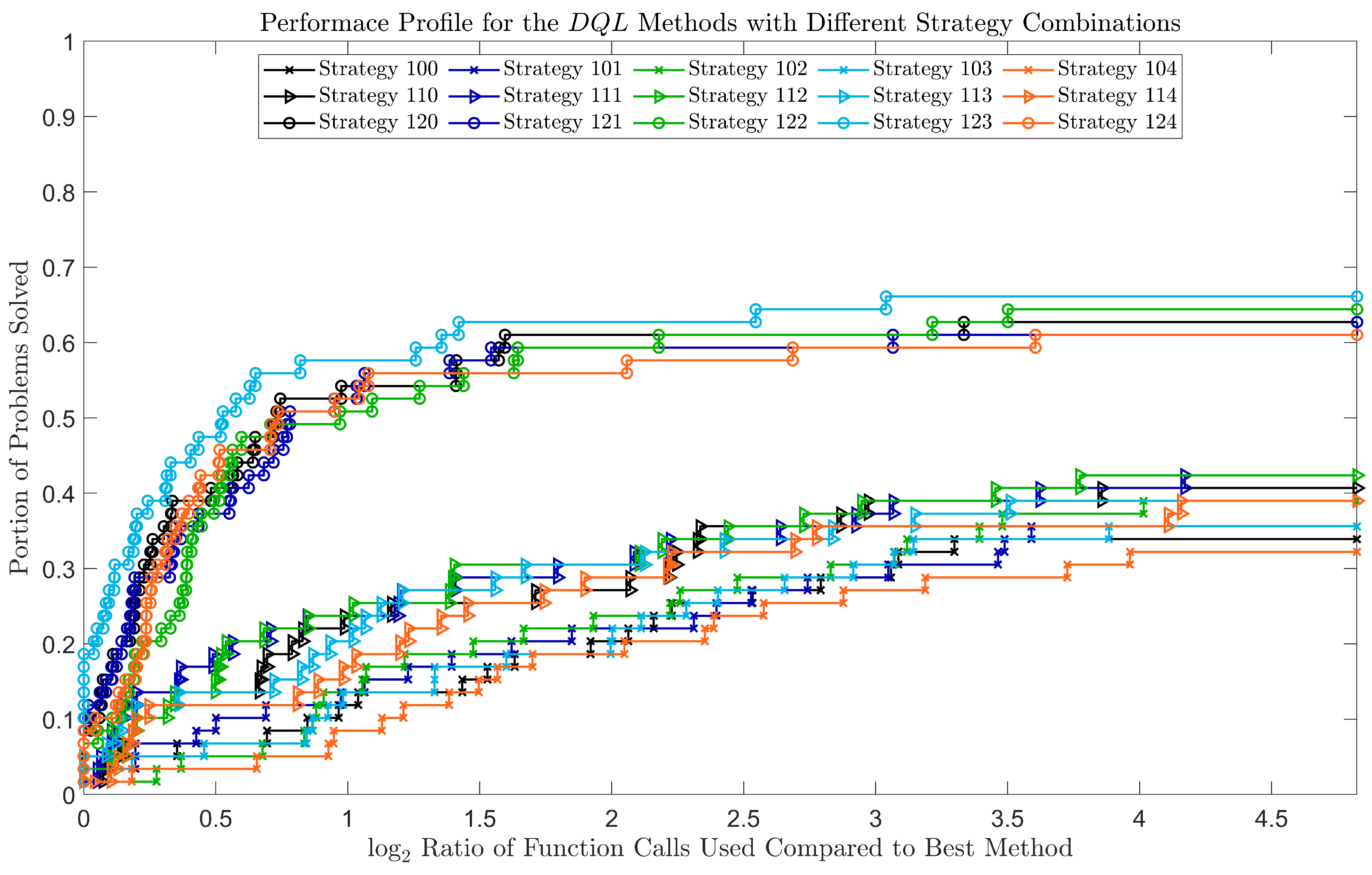
3.2.2. Performance Benchmark

We used the 59 test functions from Section 2 of [22] and [23]. These problems were transformed to the sum of square problems to fit into our code environment. The dimensions of these problems range from 2 to 20. A large portion ($26\%$) of the problems are in ${\mathbb{R}}^5$, which is identical to the first solid-tank design problem discussed in Section 5. We note that Problem 2.13 and 2.17 from [22] were omitted due to scaling problems.

The benchmarking and analysis followed the processes recommend in [24].

We first solved all the problems using the same accuracy and stability requirement by the fmincon function from Matlab. We used these solutions as a reference to the quality of our solutions. Then, we solved the problems by each strategy combination and recorded their number of function calls and the stop_flag.

Since the direct step strategy uses a random rotation, we performed each method multiple times to obtain its average performance. We denoted the function calls used by strategy combination s for problem p at trial r as $t_{s,p,r}$ and the average performance of strategy combination s for problem p as $t_{s,p}$. If a method failed at some trial, we proceeded with the next trial until a successful trial or until the evaluation budget was exhausted. If the method found a solution, then we considered the function calls it used as the summation among all the previously failed trials plus this successful trial. Therefore, the average performance of strategy combination s for problem p was defined as

$$t_{s,p}=\frac{{\sum }_r{t}_{s,p,r}}{r_{\mathrm{total}}-r_{\mathrm{fail}}},$$

(31)

where $r_{\mathrm{total}}$ is the number of total trials and $r_{\mathrm{fail}}$ is the number of failed trials.

If $t_{s,p}$ was larger than max_search, then we said that the strategy combination could not find the target solution within the evaluation budget and reset $t_{s,p}=\infty$.

We used the performance profile described in [25] to compare the performance among the strategy combinations. The performance profile first evaluated the performance ratio,

$$r_{s,p}=\frac{t_{s,p}}{min\{t_{s,p}:s\in S\}},$$

(32)

where S is the set of all strategy combinations. This ratio told us how the performance of strategy s at problem p compared to the best performance of the strategy at the problem. Then, we plotted the performance profile of strategy s as

$${\rho }_s\left(\tau \right)=\frac{1}{\left|P\right|}\left|\{p\in P:r_{s,p}\le \tau \}\right|,$$

(33)

where P is the set of all problems and $\left|·\right|$ denotes the number of elements in a set. The performance profile told us the portion of the problems solved by strategy s when the performance ratio was not greater than a factor $\tau \in \mathbb{R}$. In all results, we validated the performance profile by also creating profiles with fewer strategies to check if the switching effect occurred [26]. The switching effect never occurred.

3.2.3. Discussion on the Experiment Results

The performance profile for all the DQLstrategies is shown in Figure 2. From Figure 2, we can see that the performance profile formed three clusters. The best performing strategy combinations were strategies 123, 122, 121, 120, and 124. The underperforming strategy combinations were strategies 102, 103, 101, 100, and 104. In addition, this ranking held for any $\tau$. We therefore drew the following conclusions.

Figure 2. The performance profile for the DQL method with different strategy combinations.

• Quadratic step strategy 2 outperformed quadratic step strategy 1, which outperformed disabling the quadratic step. This showed that the quadratic step led to a performance improvement.
• Linear step strategy 4 was the worst strategy in every cluster. This strategy slowed down the performance. In addition, linear step strategies 1, 2, and 3 and disabling the linear step showed a mixed performance. Their performance differences were too small to find a clear winner.

These conclusions above gave us the insight to develop the Smart DQL method. In the Smart DQL method, we allow the method to choose the appropriate strategy dynamically and adaptively. First, since both quadratic step strategies were better than disabling the quadratic step, we decided to include both quadratic step strategies in the Smart DQL method. For the linear step strategies, we decided to remove linear step strategy 4 and we allowed the method to choose appropriate linear step strategies. In addition, we developed a better rotation strategy that selected the rotation direction using the results of previous iterations. The Smart DQL method is discussed in the next section.

4. SMART DQL Method

In this section we introduce the Smart DQL method. The Smart DQL method fits under the same framework as the DQL method. However, while the DQL method applies a static strategy, the Smart DQL method chooses the search strategies dynamically and adaptively.

4.1. Frameworks of Smart Steps

4.1.1. Smart Quadratic Step

In the smart quadratic step, we aim to combine both quadratic step strategy 1 and quadratic step strategy 2. We know that quadratic step strategy 2 performs best compared to other options, so the method should choose to perform quadratic step strategy 2 whenever the conditions are met. To perform quadratic step strategy 2, we require that both gradient and Hessian approximation at $x_0^k$ are well-defined. This can be checked by examining whether ${\nabla }_s^{2}f(x_0^k;S,\left\{{\delta }_h^j{D}_h^j\right\})\in {\mathbb{R}}^{n\times n}.$ If this does not hold, then the method should perform quadratic step strategy 1. To do so, we require that the $2n+1$ evaluated points from the previous direct step are well-defined. This can be checked by examining whether ${\nabla }_{c}f(x_0^k;{\delta }^k{D}^k)\in {\mathbb{R}}^n$. The pseudocode for the smart quadratic step is shown in Algorithm 7.

Algorithm 7 smart_Quadratic_Step (${\nabla }_{c}f(x_0^k;{\delta }^k{D}^k)$, ${\nabla }_s^{2}f(x_0^k;S,\left\{{\delta }_h^j{D}_h^j\right\})$)

1: if  ${\nabla }_s^{2}f(x_0^k;S,\left\{{\delta }_h^j{D}_h^j\right\})\in {\mathbb{R}}^{n\times n}$  then   2:     Find ${\mathbb{Q}}^k$ using quadratic step strategy 2   3: else   4:     if ${\nabla }_{c}f(x_0^k;{\delta }^k{D}^k)\in {\mathbb{R}}^n$ then   5:         Find ${\mathbb{Q}}^k$ using quadratic step strategy 1   6:     else   7:         ${\mathbb{Q}}^k\leftarrow \varphi$   8:     end if   9: end if 10: Return ${\mathbb{Q}}^k$

4.1.2. Smart Linear Step

In the smart linear step, the method should choose among the linear step strategies. Linear step strategy 4 ranked worse than disabling the linear step. Therefore, we removed linear step strategy 4 from our strategy pool. Our goal was to design an algorithm that chose among linear step strategies 1, 2, and 3 to give the method a higher chance to find an improvement at the current iterate.

We propose that when the last descent distance $∥x_0^k-x_0^s∥$ is larger than the current search step length, it is likely that the solution is even further, so the method should initiate an exploration move. Since linear step strategy 3 had better exploration ability, this strategy should be initiated under this condition. Notice that linear step strategy 2 had better exploitation ability, however, it was more computationally expensive than linear step strategy 1. Thus, linear step strategy 2 should perform better when $x_0^k$ is close to an approximate solution and linear step strategy 1 should perform better when $x_0^k$ is still far away from an approximate solution. The comparison between ${ϵ}_{\mathrm{MAX}\_\mathrm{STEP}}$ and the search step length is a good indicator for this situation. When the search step length was smaller than ${ϵ}_{\mathrm{MAX}\_\mathrm{STEP}}$, we found that $x_0^k$ was close to an approximate solution, so spending more effort on local exploitation, i.e., using linear step strategy 2, might give the better result. In the case when the search step length is larger than ${ϵ}_{\mathrm{MAX}\_\mathrm{STEP}}$, the method should spend less computational power on local exploitation. In some case, such as the first iteration, the conditions for any of above the linear step strategies do not hold. In this case, the linear step is disabled. The pseudocode for the smart linear step is shown in Algorithm 8.

Algorithm 8 smart_linear_step ($x_0^k$, $x_0^s$, ${\nabla }_{c}f(x_0^k;{\delta }^k{D}^k)$)

1: if$k\ge 2$ and $∥x_0^k-x_0^s∥\ge {\delta }^k$ then   2:     Find ${\mathbb{L}}^k$ using linear step strategy 3   3: else   4:     if ${\nabla }_{c}f(x_0^k;{\delta }^k{D}^k)\in {\mathbb{R}}^n$ then   5:         if ${\delta }^k\le {ϵ}_{\mathrm{MAX}\_\mathrm{STEP}}$ then   6:            Find ${\mathbb{L}}^k$ using linear step strategy 2   7:         else   8:            Find ${\mathbb{L}}^k$ using linear step strategy 1   9:         end if 10:     else 11:         ${\mathbb{L}}^k\leftarrow \varphi$ 12:     end if 13: end if 14: Return ${\mathbb{L}}^k$

4.1.3. Smart Direct Step

In the smart direct step, we aimed to design a rotation strategy that outperformed random rotation. Particularly, this smart direct step should be a deterministic strategy such that the method returns the same result for the same problem setup. To design such an algorithm, we first studied the results from a successful or failed direct, quadratic, or linear step.

A successful direct step skips both quadratic and linear step and proceeds with the direct step in the next iteration. In this case, the same search directions should be used because these directions have proven to be successful.

If the direct step fails, then the method proceeds with the quadratic step. For both quadratic step strategies, the method builds a quadratic model. If the quadratic step succeeds, then it is likely that this quadratic model is accurate. Therefore, the method uses the gradient of this model as desired rotation direction for the direct step.

If the gradient of the quadratic model was 0, then the quadratic step would fail. If the quadratic step fails, then the method proceeds with the linear step. For any linear step strategy, if the linear step succeeds, then the direction used in the linear step is likely to be a good descent direction. Therefore, the direct step uses the same direction as the previous linear step as the desired direction. Otherwise, if the linear step fails, then we know that the linear step direction at $x_0^k$ is a nondecreasing direction. Therefore, at iteration $k+1$, the linear step direction at $x_0^{k+1}$ is set as an undesired direction.

Algorithm 9 provides the pseudocode of the process to determine $r^k$ in the direct step. Note that since the linear step decision process requires information from the previous iteration, at the first iteration, the method uses the coordinate direction as the desired direction.

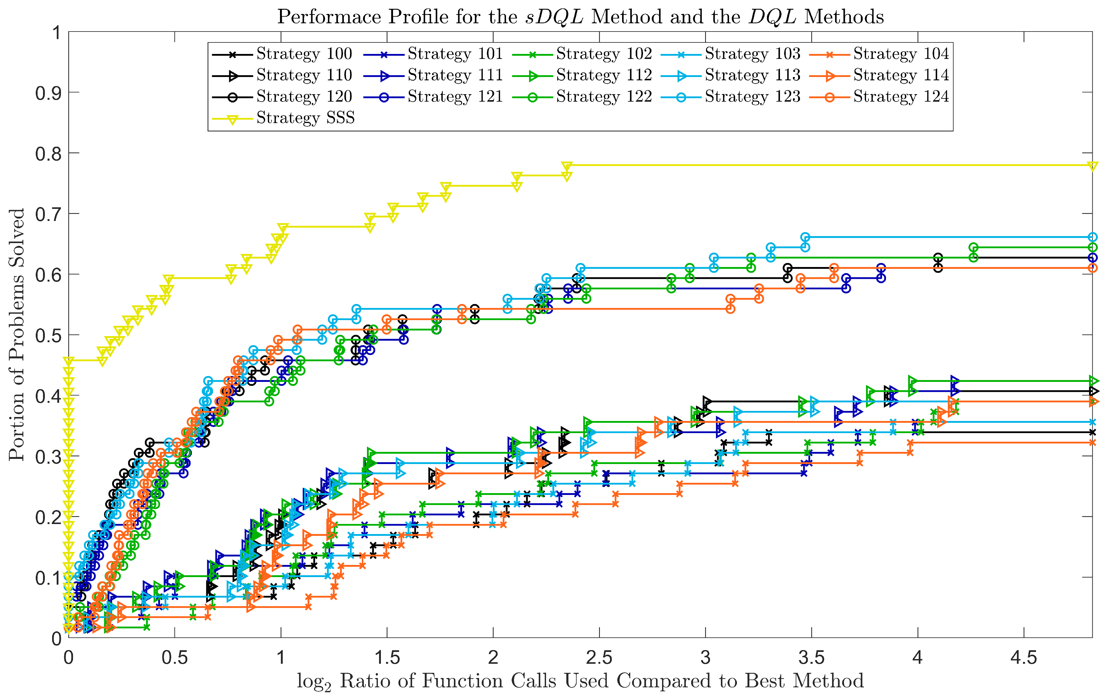
4.2. Benchmark for Smart DQL Method

4.2.1. Experiment Result

We marked the smart strategy as strategy S, so the strategy SSS of the DQL method is the Smart DQL method. We performed the numerical experiment with the same setup as the benchmark for the step strategies from the previous section. Then, we constructed the performance profile as shown in Figure 3.

Algorithm 9 Determine_Rotation_Direction ( $D^{k-1}$, $m^{k-1}\left(x\right)$, $d^{k-1}$)

1: if  $k=1$  then   2:       $r^k=e_1$ is a desired direction   3: else   4:       if the direct step at iteration $k-1$ succeeds then   5:             $r^k=r^{k-1}$   6:       else   7:             if the quadratic step at iteration $k-1$ succeeds then   8:                    if $\nabla m^{k-1}\left(x_0^k\right)=0$ then   9:                          $r^k=e_1$ is a desired direction 10:                    else 11:                          $r^k=\nabla m^{k-1}\left(x_0^k\right)$ is a desired direction 12:                    end if 13:             else 14:                    if the linear step at iteration $k-1$ succeeds then 15:                          $r^k=d^{k-1}$ is a desired direction 16:                    else 17:                          $r^k=d^{k-1}$ is an undesired direction 18:                    end if 19:             end if 20:       end if 21: end if 22: Return $r^k$

Figure 3. The performance profile for the Smart DQL method and all the DQL methods.

4.2.2. Discussion

As we can see from Figure 3, the Smart DQL method preformed best at any given $\tau$. The Smart DQL method solved more than $45\%$ of the problems as the fastest method. In addition, it solved more than $75\%$ of the problems, which was more than any DQL method. Therefore, we attained a considerable improvement over the original DQL method. In the next section, we apply the Smart DQL method in a real-world application.

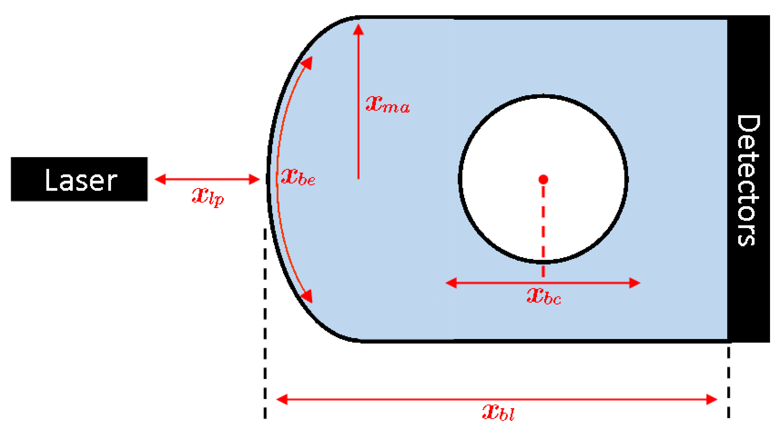
5. Solid-Tank Design Problem

5.1. Background

The solid-tank design problem [16] aims to create a design for a solid-tank fan-beam optical CT scanner with minimal matching fluid, while maximizing light collection, minimizing image artifacts, and achieving a uniform beam profile, thereby maximizing the usable dynamic range of the system. For a given geometry, a ray-path simulator designed by the UBCO gel dosimetry group is available in MATLAB and outputs tank design quality scores. The simulator is computationally expensive, so the efficiency of the method is crucial for solving this problem.

In the original problem, there are five parameters that control the geometry design. As shown in Figure 4, these are block length $x_{bl}$, bore position $x_{bc}$, fan-laser position $x_{lp}$, lens block face’s semi-major axis length $x_{ma}$, and the lens block face’s eccentricity $x_{be}$.

Figure 4. The geometry of the solid-tank fan-beam optical CT scanner.

These parameters give us an input $x\in {\mathbb{R}}^5$. The following bounds are the constraints for the problem.

$$\begin{array}{cc}\hfill x={\left[\begin{array}{ccccc}{x}_{bl}& x_{bc}& x_{lp}& x_{ma}& x_{be}\end{array}\right]}^{\top }& \in {\mathbb{R}}^5\hfill \end{array}$$

(34)

$$\begin{array}{cc}\hfill x_{bl}& \le 400\hfill \end{array}$$

(35)

$$\begin{array}{cc}\hfill x_{bl}& \ge 2l+2|x_{bc}|\hfill \end{array}$$

(36)

$$\begin{array}{cc}\hfill x_{bc}& \in [-30,30]\hfill \end{array}$$

(37)

$$\begin{array}{cc}\hfill x_{lp}& \in [40,100]\hfill \end{array}$$

(38)

$$\begin{array}{cc}\hfill x_{ma}& \in [40,80]\hfill \end{array}$$

(39)

$$\begin{array}{cc}\hfill x_{be}& \in [0,1],\hfill \end{array}$$

(40)

where $l=$ 52 mm (bore radius) + 5 mm (safeguard distance). The parameters $x_{bl},x_{bc},x_{lp}$, and $x_{ma}$ are in mm and $x_{be}$ is dimensionless.

An advanced version of the simulation software tool is currently being developed. This version introduces three new variables ($x_{be2},x_{ecc2}\mathrm{and}{x}_{d3}$), resulting in an eight-variable problem with the following constraints.

$$\begin{array}{cc}\hfill x={\left[\begin{array}{cccccccc}{x}_{bl}& x_{bc}& x_{lp}& x_{ma}& x_{be}& x_{be2}& x_{ecc2}& x_{d3}\end{array}\right]}^{\top }& \in {\mathbb{R}}^8\hfill \end{array}$$

(41)

$$\begin{array}{cc}\hfill x_{bl}& \in [2l+2|x_{bc}|,400]\hfill \end{array}$$

(42)

$$\begin{array}{cc}\hfill x_{bc}& \in [-40,40]\hfill \end{array}$$

(43)

$$\begin{array}{cc}\hfill x_{lp}& \in [40,100]\hfill \end{array}$$

(44)

$$\begin{array}{cc}\hfill x_{ma}& \in [40,160]\hfill \end{array}$$

(45)

$$\begin{array}{cc}\hfill x_{be}& \in [0,1]\hfill \end{array}$$

(46)

$$\begin{array}{cc}\hfill x_{be2}& \in [70,120]\hfill \end{array}$$

(47)

$$\begin{array}{cc}\hfill x_{ecc2}& \in [0,2.5]\hfill \end{array}$$

(48)

$$\begin{array}{cc}\hfill x_{d3}& \in [0,400-x_{bl}],\hfill \end{array}$$

(49)

where $l=$ 52 mm (bore radius) + 5 mm (safeguard distance). The parameters $x_{bl},x_{bc},x_{lp}$, $x_{ma}$, $x_{be2}$, and $x_{d3}$ are in mm and $x_{be}$ and $x_{ecc2}$ are dimensionless.

At this time, the five-variable model is ready for public use. The eight-variable model is still undergoing detailed physics validation, but will be released along with the solid-tank simulation software tool. (See Data and Software Availability Statement for release details.)

In this section, we optimize the solid-tank design problems using the DQL and Smart DQL methods.

5.2. Transforming the Optimization Problem

We defined $f_{simu}:{\mathbb{R}}^n\to \mathbb{R}$ as the simulating scores at a given geometry, where $n=5$ for the original problem and $n=8$ for the redesigned problem. The output was normalized to give a final value between zero and one. Since the DQL and Smart DQL methods were designed for minimizing unconstrained problems, we transformed the problems as follows,

$$-min\left\{-f_{simu}\left({\mathrm{Proj}}_C\left(x\right)\right):x\in {\mathbb{R}}^n\right\}$$

(50)

where ${\mathrm{Proj}}_C\left(x\right)$ is the projection of the input x onto the constraints C. For ease of interpretation, we shall report the optimized results as a value between zero and one with the goal of maximizing this value.

5.3. Experiment Result and Discussion

The stopping parameters for the solid-tank design problems are shown in Table 3; all other parameters remained the same as in Table 2. The maximum accepted step length ${ϵ}_{\mathrm{MAX}\_\mathrm{STEP}}$ was designed to be the target manufacturing accuracy of the design. The minimum accepted step length ${ϵ}_{\mathrm{MIN}\_\mathrm{STEP}}$ was designed to be the manufacturing error of the design. ${ϵ}_{\nabla }$ ensured the accuracy of the stability of the solution to be within ${10}^{-3}$.

Table 3. The Stopping Parameters for the Solid-Tank Design Problems.

Parameter	Value
${ϵ}_{\nabla }$	$2\times {10}^{-3}$
${ϵ}_{\mathrm{MAX}\_\mathrm{STEP}}$	$0.5$
${ϵ}_{\mathrm{MIN}\_\mathrm{STEP}}$	$0.001$
max_search ($n=5$)	5000
max_search ($n=8$)	8000

For each experiment, the method was assigned a random initial point within the constraints. Then, if the method was able to find a solution with unused function calls, it was assigned with a new initial point and began a new search. This process was repeated until the evaluation budget was exhausted.

Each experiment was performed with three different profile settings: water, FlexyDos3D, and ClearView^TM. These represented three standard dosimeters used in gel dosimetry and each had unique optical parameters (index of refraction and linear attenuation coefficient). As such, we had six related but distinct case problems.

To compare the performance of the DQL and Smart DQL methods, we ran the experiment with both methods. For each individual case, both methods were assigned the same list of initial points and evaluation budget. The optimum scores found by different methods for distinct profiles are shown in Table 4. Recall that values were between zero and one with the goal of maximizing these values.

Table 4. Optimum Scores for Solid-Tank Design Problem.

Dimension	Method	Water	FlexyDos3D	ClearViewTM
		${\mathbf{r}}^{\mathbf{1}}=\mathbf{1}.\mathbf{3316}$	$\mathbf{r}=\mathbf{1}.\mathbf{4225}$	$\mathbf{r}=\mathbf{1}.\mathbf{3447}$
$n=5$	DQL	0.801	0.979	0.952
$n=5$	Smart DQL	0.829	0.981	0.956
$n=8$	DQL	0.767	0.977	0.686
$n=8$	Smart DQL	0.857	0.974	0.831

¹ The index of refraction of the corresponding dosimeter.

Among the six individual tests, the Smart DQL method found a solution with a higher score for five of them under the same evaluation budget and initial points. In two cases ($n=8$ water and $n=8$ ClearView^TM), the Smart DQL method found a significant improvement. For the only case where DQLreturned a higher score ($n=8$ FlexyDos3D), the improvement was only 0.003. This showed that the Smart DQL method was more reliable in this application than the DQL method. The experiment results agreed with our conclusion from the performance benchmark.

We show the optima from the Smart DQL method in Table 5 and Table 6 for the five- and eight-variable models, respectively.

Table 5. Optima for Solid-Tank Design Problem ($n=5$).

	${\mathit{x}}_{\mathit{bl}}$	${\mathit{x}}_{\mathit{bc}}$	${\mathit{x}}_{\mathit{lp}}$	${\mathit{x}}_{\mathit{ma}}$	${\mathit{x}}_{\mathit{be}}$
Profile	(mm)	(mm)	(mm)	(mm)
Water	252.4	19.2	71.8	70.1	0
FlexyDos3D	282.0	5.8	51.8	67.0	0
ClearViewTM	225.1	21.2	63.1	69.0	0

Table 6. Optima for Solid-Tank Design Problem ($n=8$).

	${\mathit{x}}_{\mathit{bl}}$	${\mathit{x}}_{\mathit{bc}}$	${\mathit{x}}_{\mathit{lp}}$	${\mathit{x}}_{\mathit{ma}}$	${\mathit{x}}_{\mathit{be}}$	${\mathit{x}}_{\mathit{be}2}$	${\mathit{x}}_{\mathit{ecc}2}$	${\mathit{x}}_{\mathit{d}3}$
Profile	(mm)	(mm)	(mm)	(mm)		(mm)		(mm)
Water	122.6	−4.3	94.0	79.8	0.8	70.0	0	23.4
FlexyDos3D	114.0	0	100.0	68.3	0.1	70.0	0	0.5
ClearViewTM	114.0	0	100.0	93.3	1.0	70.8	0.3	46.1

We were not able to identify a uniform design that was competitive for all profiles. The optimal design of the solid tank varied for different models and among different profiles. We noticed that in the eight-variable design, the method tried to minimize the block length $x_{bl}$ and maximize the laser position $x_{lp}$ for both FlexyDos3D and ClearView^TM; this suggested that further improvement may be gained by extending the range for these parameters.

6. Conclusions

In this research, we presented a DFO framework that allowed for direct search methods and model-based methods to be united into a single algorithm.

The DQLframework showed advantages over other methods in the literature. First, unlike heuristic based methods, convergence was mathematically proven under reasonable assumptions. Second, unlike more rigid DFO methods, the DQLframework was flexible, allowing the combination of direct search, quadratic step, and linear step methods into a single algorithm. This balance of mathematical rigour and algorithmic flexibility created a framework with a high potential for future use.

The algorithm was further examined numerically. In particular, we benchmarked the developed DQL method’s strategy combinations to determine the optimal combination. The benchmark implied that there was no obvious winner. This motivated the development of the Smart DQL method. We presented the pseudocode for the Smart DQL method and conducted an additional benchmark. The Smart DQL method outperformed all other DQL methods in the benchmark. Last, the Smart DQL method was used to solve the solid-tank design problem. The Smart DQL method was able to produce higher-quality solutions for this real-world application compared to the DQL method, which verified the high performance of the decision-making mechanism.

While the DQL and Smart DQL methods both balanced mathematical rigour and algorithmic flexibility, it is worth noting their drawbacks. The most notable one is that the implementations of DQL and Smart DQL are both at the prototype stage. In comparison to more mature implementations (such as that of SID-PSM [13]), DQL and Smart DQL are unlikely to compete at this time. Another drawback is the need to asymptotically focus on direct search to ensure convergence. Further study will work to advance the Smart DQL method both in the quality of its implementation and the requirements for convergence.

References

- Ali, E.; Abd Elazim, S.; Balobaid, A. Implementation of coyote optimization algorithm for solving unit commitment problem in power systems. Energy 2023, 263, 125697. [Google Scholar] [CrossRef]
- Abd Elazim, S.; Ali, E. Optimal network restructure via improved whale optimization approach. Int. J. Commun. Syst. 2021, 34, e4617. [Google Scholar]
- Ali, E.; Abd Elazim, S. Mine blast algorithm for environmental economic load dispatch with valve loading effect. Neural Comput. Appl. 2018, 30, 261–270. [Google Scholar] [CrossRef]
- Alarie, S.; Audet, C.; Garnier, V.; Le Digabel, S.; Leclaire, L.A. Snow water equivalent estimation using blackbox optimization. Pac. J. Optim. 2013, 9, 1–21. [Google Scholar]
- Gheribi, A.; Audet, C.; Le Digabel, S.; Bélisle, E.; Bale, C.; Pelton, A. Calculating optimal conditions for alloy and process design using thermodynamic and property databases, the FactSage software and the Mesh Adaptive Direct Search algorithm. Calphad 2012, 36, 135–143. [Google Scholar] [CrossRef]
- Gheribi, A.; Pelton, A.; Bélisle, E.; Le Digabel, S.; Harvey, J.P. On the prediction of low-cost high entropy alloys using new thermodynamic multi-objective criteria. Acta Mater. 2018, 161, 73–82. [Google Scholar] [CrossRef]
- Marwaha, G.; Kokkolaras, M. System-of-systems approach to air transportation design using nested optimization and direct search. Struct. Multidiscip. Optim. 2015, 51, 885–901. [Google Scholar] [CrossRef]
- Chamseddine, I.M.; Frieboes, H.B.; Kokkolaras, M. Multi-objective optimization of tumor response to drug release from vasculature-bound nanoparticles. Sci. Rep. 2020, 10, 1–11. [Google Scholar] [CrossRef]
- Conn, A.; Scheinberg, K.; Vicente, L. Introduction to Derivative-Free Optimization; SIAM: Philadelphia, PA, USA, 2009. [Google Scholar]
- Audet, C.; Hare, W. Derivative-Free and Blackbox Optimization; Springer: Cham, Switzerland, 2017. [Google Scholar]
- Audet, C. A survey on direct search methods for blackbox optimization and their applications. In Mathematics without Boundaries; Springer: Berlin/Heidelberg, Germany, 2014; pp. 31–56. [Google Scholar]
- Hare, W.; Nutini, J.; Tesfamariam, S. A survey of non-gradient optimization methods in structural engineering. Adv. Eng. Softw. 2013, 59, 19–28. [Google Scholar] [CrossRef]
- Custodio, A.L.; Vicente, L.N. SID-PSM: A Pattern Search Method Guided by Simplex Derivatives for Use in Derivative-Free Optimization; Departamento de Matemática, Universidade de Coimbra: Coimbra, Portugal, 2008. [Google Scholar]
- Custódio, A.L.; Rocha, H.; Vicente, L.N. Incorporating minimum Frobenius norm models in direct search. Comput. Optim. Appl. 2010, 46, 265–278. [Google Scholar] [CrossRef]
- Manno, A.; Amaldi, E.; Casella, F.; Martelli, E. A local search method for costly black-box problems and its application to CSP plant start-up optimization refinement. Optim. Eng. 2020, 21, 1563–1598. [Google Scholar] [CrossRef]
- Ogilvy, A.; Collins, S.; Tuokko, T.; Hilts, M.; Deardon, R.; Hare, W.; Jirasek, A. Optimization of solid tank design for fan-beam optical CT based 3D radiation dosimetry. Phys. Med. Biol. 2020, 65, 245012. [Google Scholar] [CrossRef] [PubMed]
- Hare, W.; Jarry–Bolduc, G.; Planiden, C. Error bounds for overdetermined and underdetermined generalized centred simplex gradients. arXiv 2020, arXiv:2006.00742. [Google Scholar] [CrossRef]
- Hare, W.; Jarry-Bolduc, G.; Planiden, C. A matrix algebra approach to approximate Hessians. Preprint 2022. Available online: https://www.researchgate.net/publication/365367734_A_matrix_algebra_approach_to_approximate_Hessians (accessed on 7 November 2021).
- Masson, P. Rotations in Higher Dimensions. 2017. Available online: https://analyticphysics.com/Higher%20Dimensions/Rotations%20in%20Higher%20Dimensions.htm (accessed on 7 November 2021).
- MathWorks. MATLAB Version 2020a. Available online: https://www.mathworks.com/products/matlab.html (accessed on 15 November 2021).
- Mifflin, R.; Strodiot, J.J. A bracketing technique to ensure desirable convergence in univariate minimization. Math. Program. 1989, 43, 117–130. [Google Scholar] [CrossRef]
- Lukšan, L.; Vlcek, J. Test problems for nonsmooth unconstrained and linearly constrained optimization. Tech. Zpráva 2000, 798, 5–23. [Google Scholar]
- Moré, J.; Garbow, B.; Hillstrom, K. Testing unconstrained optimization software. ACM Trans. Math. Softw. (TOMS) 1981, 7, 17–41. [Google Scholar] [CrossRef]
- Beiranvand, V.; Hare, W.; Lucet, Y. Best practices for comparing optimization algorithms. Optim. Eng. 2017, 18, 815–848. [Google Scholar] [CrossRef]
- Dolan, E.; Moré, J. Benchmarking optimization software with performance profiles. Math. Program. 2002, 91, 201–213. [Google Scholar] [CrossRef]
- Gould, N.; Scott, J. A note on performance profiles for benchmarking software. ACM Trans. Math. Softw. (TOMS) 2016, 43, 1–5. [Google Scholar] [CrossRef]
Disclaimer/Publisher’s Note: The statements, opinions and data contained in all publications are solely those of the individual author(s) and contributor(s) and not of MDPI and/or the editor(s). MDPI and/or the editor(s) disclaim responsibility for any injury to people or property resulting from any ideas, methods, instructions or products referred to in the content. |
© 2023 by the authors. Licensee MDPI, Basel, Switzerland. This article is an open access article distributed under the terms and conditions of the Creative Commons Attribution (CC BY) license (https://creativecommons.org/licenses/by/4.0/).