Abstract
Importance sampling, a variant of online sampling, is often used in neural network training to improve the learning process, and, in particular, the convergence speed of the model. We study, here, the performance of a set of batch selection algorithms, namely, online sampling algorithms that process small parts of the dataset at each iteration. Convergence is accelerated through the creation of a bias towards the learning of hard samples. We first consider the baseline algorithm and investigate its performance in terms of convergence speed and generalization efficiency. The latter, however, is limited in case of poor balancing of data sets. To alleviate this shortcoming, we propose two variations of the algorithm that achieve better generalization and also manage to not undermine the convergence speed boost offered by the original algorithm. Various data transformation techniques were tested in conjunction with the proposed scheme to develop an overall training method of the model and to ensure robustness in different training environments. An experimental framework was constructed using three naturally imbalanced datasets and one artificially imbalanced one. The results assess the advantage in convergence of the extended algorithm over the vanilla one, but, mostly, show better generalization performance in imbalanced data environments.
1. Introduction
The rapid growth of deep learning in recent years is being attributed to the vast development of hardware capabilities, as well as the abundance of available training data. Specifically, the latter is extremely important for the training process of a deep learning model. The vast quantity of data is very helpful for a neural network to achieve a good generalization performance, but the particularities of the data also play a significant role. One basic trait of a dataset is its underlying distribution and its divergence with the theoretical (perfect) distribution of the task at hand. Sometimes, this distribution suffers from imbalances that can make the training of a network difficult, but, more importantly, it can affect, negatively, its generalization performance [1,2]. A distribution can be balanced when the amount of samples per different and unique observations in a dataset is uniformly distributed. This issue has been referred to in the literature as class imbalance in the context of a classification problem.
Usually, in a dataset that exhibits some imbalance, there exists two types of classes. There are the classes with a plethora of observations, named majority classes, and classes with a lack of observations, named minority classes. This phenomenon appears quite often in real world datasets and tasks due to various reasons; the most common one being the existence of rare instances of a specific sample that holds great interest for the specific problem. For example, in the field of fraud detection (i.e., fraudulent creditcard detection), there can be many legal transactions with credit cards and only a handful where a fraud actually occurs. However, these rare instances are the backbone of the said task and what a machine learning algorithm should strive to learn. How the model learns to distinguish between majority and minority classes is the objective of a wide variety of techniques that battle against this imbalance.
There are various methods that tackle the data imbalance problem, many of which are discussed in the Related Work section (Section 2). In this work, we are going to elaborate on Batch Selection with Biased Sampling (BSBS), a sampling method used for faster convergence, which was originally introduced in [3]. The method focused on balanced datasets and tried to improve the training process by giving more attention to harder samples. However, in the real world, the vast majority of datasets are imbalanced. In this paper, we are going to examine these kind of datasets and propose two variations to the main BSBS algorithm.These extensions endow BSBS with higher generalization performance on imbalanced datasets. In the experimental part of the paper, we utilize multiple data transformation methods to test the algorithm on different aspects of the same dataset. It is also shown that a hybrid method combining these data-transformation techniques with the enhanced BSBS approach behaves best as far as generalization performance is concerned.
The main contributions of this paper can be summarized in the following points:
- A novel set of algorithms consisting of the original BSBS scheme that achieve better F1-score and balanced accuracy on four different imbalanced datasets.
- An analysis of 11 different data-transformation methods and their interaction with the proposed batch selection algorithms, as well as a comparison with 2 state-of-the-art online sampling methods.
- The proposal of a hybrid method that combines the proposed algorithms with the best data transformation techniques, without affecting the convergence rate of the original algorithm.
The rest of the paper is structured as follows. Section 2 presents related work and Section 3 describes the new methodologies used in this paper. Section 4 outlines the experimental framework, where all the aforementioned techniques are tested. Results are displayed and discussed in Section 5. Finally, conclusions and further research are summarized in Section 6.
2. Related Work
In this section, we are going to discuss some popular methods regarding imbalance, some of which are going to be employed later on during the experiments. The advantages and disadvantages of each method are going to be highlighted, along with our contribution in the literature. The methods for addressing dataset imbalance are mainly divided into two main categories. The first type involves transforming the dataset and its underlying distribution into a more balanced state. The second is based around the learning algorithm (i.e., classifier) and the way it tackles the imbalance without changing the training dataset. Both types of methods have been used in the literature in various ways, some of which will be described below.
The most common techniques to tackle imbalance are dataset transformation methods. Their goal is to change the structure of the dataset by adding, removing, or transforming samples of the dataset in order to make it easier for models to learn to distinguish the minority classes. Such techniques are oversampling, undersampling, and the combination of the two, all of which are discussed in what follows.
Oversampling is one of the most popular techniques that address imbalance. Random oversampling (ROS) is the most simple version of it, where the samples of the minority classes are duplicated multiple times in order to reach the number of samples of the majority classes. It is a method that does not require any heavy computational cost and can be used successfully alongside deep learning networks, as well as many classical machine learning techniques. However, there are some disadvantages of ROS. The main drawback occurs when the minority classes display very low diversity. This happens in situations of extreme imbalance, when the number of samples of the minority class is very low. The multiple replications of the small in variety minority classes leave the overall distribution far from a realistic one, which may lead to overfitting. Various techniques have been developed to alleviate this issue. One of the most used is SMOTE [4]. This method utilizes the k-nearest neighbors (k-NN) algorithm [5] to select similar samples of the minority classes and constructs new samples randomly by mixing them together. Thus, SMOTE produces new synthetic data that enrich the dataset altering the underlying distribution to a more realistic one. Many variants of SMOTE have developed over the years. Borderline-SMOTE [6] is a variant that strives to improve the oversampling process by selecting samples that lie close to the border of each class. These samples are more apt to be misclassified than samples far from the borderline. Thus, borderline-SMOTE finds the borderline examples of the minority classes and oversamples them. Another recent variant of SMOTE is the K-means-SMOTE [7], which utilizes the K-means algorithm to divide the samples into clusters. Then, it selects the clusters with the greater imbalance and computes a sampling weight for each cluster. The sampling weight is later used to calculate the number of new samples to be generated from the minority classes for each of the selected clusters. The sampling, finally, is performed using the SMOTE algorithm. Another useful oversampling technique is Adasyn [8], which is considered an improvement of SMOTE, as it uses k-NN to find k neighbor samples of each minority sample. However, the difference lies in the amount of samples that are generated. Adasyn calculates the number of samples to be generated based on the distribution of the neighborhood of each minority sample.
Undersampling is the other popular data transformation technique that tackles imbalance. In contrast to oversampling, undersampling removes samples from the majority class. Specifically, the simplest algorithm, random undersampling (RUS), selects samples from the majority classes at random and removes them until both majority and minority classes have the same amount of samples. In general, undersampling is considered worse compared to oversampling because deep learning techniques work better with more data. However, there are cases where undersampling can outperform oversampling [9]. Another undersampling algorithm is the Edited Nearest Neighbors (ENN) [10]. ENN uses the k-NN algorithm to find the neighbors of all the samples of the majority classes. Then, it removes the samples, wherein the majority of their neighbors belong to a different class. In other words, it removes samples from the majority classes that lie close to the borderline of classes. Tomek links [11] is another undersampling algorithm similar to ENN. The goal of this method is to find the Tomek links in the dataset and remove them. The definition of a Tomek link is a pair of two samples, one belonging in the majority and one in the minority class, wherein both are the closest neighbor of the other. Removing them, the borders of each class are easier for a model to learn and, as a result, improve the classification performance. An undersampling method that utilizes data clustering is ClusterCentroids [12], which keeps N samples from the majority class by performing a N-means clustering of the majority class and keeping the N centroids as the new majority samples.
An interesting concept that is often beneficial for imbalanced datasets is to combine the two aforementioned methods, undersampling and oversampling, in an effort of utilizing their individual advantages. This can successfully create a dataset that makes it easier for a model to learn the underlying distribution of the task. With oversampling, more samples of the minority class are added to the dataset, and, while using undersampling, a part of the majority class is removed in order to make it clearer to distinguish each class better. In this work, we will look into two such algorithms, SMOTETomek [13] and SMOTEENN [14]. Both methods, firstly, use SMOTE to oversample the minority classes and, then, use Tomek links and ENN, respectively, to clean up the majority classes. It is shown in various cases that this combination of under- and oversampling is performing better than using just one of the two [15].
Apart from the dataset transformation methods, there is another way to tackle imbalance, and that is through the learning algorithm. In other words, the goal is to construct algorithms (classifiers) that pay more attention to the minority classes in order to balance out the disparity in training data. These methods usually take a different approach during training or adjust the inference accordingly while keeping the dataset the same. Below are outlined some widely used algorithmic methods for imbalance.
One of the most common algorithmic methods is cost-sensitive learning [16], whose main focus is to create models that pay more attention to minority classes to boost the model’s performance towards them. This can be achieved in various ways that depend on the nature of the classifier at hand. Regarding neural networks [17], this is usually referred to as class weights. These weights are included in the computation of the loss function, so that samples of the minority classes, with higher class weight, affect the total loss more. Trying to minimize such loss function, the network eventually learns to display smaller error regarding the minority classes. However, apart from the loss function, cost-sensitive learning can be applied to the optimization update of the neural network. For example, the learning rate or the gradients can be adapted in order to help the model learn the minority samples.
In recent years, the development of very deep neural networks trained on large datasets has brought to light an obstacle. It is becoming very difficult to process the dataset all at once. This is where online training methods come into play. Specifically, regarding the imbalance problem, instead of transforming the large dataset with under- or oversampling, it is better to sample small parts of the dataset to be processed by the model at each training iteration. In neural networks, this is usually manifested with the use of batches (small parts of the dataset), which are used for the training update. Online Sampling can be beneficial for various reasons and can be implemented in different ways, some of which will be discussed below.
An interesting attempt at online sampling (OS) was curriculum learning [18], which was inspired by human behavior. The basic concept is to choose easy samples at the start of the training procedure and slowly keep introducing harder ones, as a human would. This results in significant improvement of the training. Later, an advancement was made with automated curriculum learning [19], where a policy defines the order of the samples being fed to the network as training inputs. The trained policy is modified to minimize the loss of the model. Beneficial, though, can also be the opposite idea of curriculum learning. It was introduced with hard example mining [20], which focuses on selecting harder samples for the network to learn in order to obtain trained faster due to the greater gradients. Online sampling is, also, called batch selection in the context of neural networks. In [21], an algorithm is presented that follows the general concept of hard example mining (focusing on hard-to-learn samples during training). Each sample has a probability to be selected in the current batch proportional to its loss. Consequently, samples with greater loss have better chances of being selected into the batch and, as a result, into the training process. Our approach is based on this idea and develops it further to be more efficient training-wise as well as performance-wise.
In general, online sampling is primarily used to boost the convergence speed of neural networks. In other words, it greatly improves the training performance of the model. Importance sampling, a variant of OS, shows great promise in accelerating the training of deep neural networks [22,23,24,25]. Important sampling can also help in reducing the variance of the updates (i.e., SGD) [26], which affects positively the optimization performance of the network. However, with respect to the scope of imbalance, the training performance (e.g., training loss) is not the primary objective; instead, the validation metric is how well the model can generalize training with the imbalanced dataset. In [27], it is shown that sampling and weighting samples by difficulty can be very effective for the validation performance of a model as well. This indicates that OS can help alleviate the imbalance problem and train better models. In [28], the authors train neural networks with a bilevel optimization scheme, which improves model fairness. Another recent approach is submodular batch selection [29], which is based on submodular function maximization and produces state-of-the-art results in various setups.
In image classification, an important technique for improved generalization performance is data augmentation. This is a method similar to online sampling, which focuses on creating new images by changing the original ones at the step of sampling during training. Augmentation can help alleviate the problems of imbalanced datasets by creating new samples of the minority class. Many works have been developed over the years around augmentation on imbalanced datasets [30,31] and have been used in various applications [32,33].
Finally, it is important to note that it is possible to combine most of the techniques that are mentioned above. Every type of such methods offers something different to the training process. Thus, hybrid methods try to construct a combination of these methods that can achieve better results than each individual method alone. A popular approach is ensembling. For example, SMOTEBoost [34] is a mix of SMOTE oversampling and boosting. Another similar hybrid method is RUSBoost [35], which, instead of SMOTE, utilizes the RUS algorithm. Apart from boosting, bagging can also be combined with imbalance techniques [36]. In [37], two hybrid methods, EasyEnsemble and BalanceCascade, are presented, which use undersampled datasets with a set of classifiers applying the concept of ensembling.
All the aforementioned methods have been used in various applications and display different advantages and disadvantages. Below, Table 1 summarizes some basic advantages and disadvantages of the general methods that are described in this section. Our approach belongs to the algorithm-based methods, but is able to work in conjunction with the data transformation ones for increased performance. The proposed algorithm tries to be scalable to bigger datasets while needing less preprocessing (advantages of online sampling), but, at the same time, it strives to incorporate some of the advantages of oversampling and undersampling (removal of redundant samples, creation of synthetic data).

Table 1.
Advantages and disadvantages of all the methods in literature.
3. Methodology
In this section, we present batch selection with the biased sampling (BSBS)algorithm, along with its two variants. The overall approach builds upon the concept that, if a model gives more attention to harder samples, convergence speed will be increased. Our aim is to derive enhanced extensions of the algorithm, that—in addition to convergence acceleration—will boost generalization efficiency regarding the imbalance problem.
3.1. Batch Selection with Biased Sampling
An original version of the BSBS approach appeared in [3]. Training of a neural network can be formulated as a non-convex optimization problem aiming to minimize a loss function. Given a dataset, the optimization goal is to minimize the sum of the losses across all data samples. The training process usually consists of two steps that are repeated through a certain number of epochs:
- Sampling a batch of samples according to a distribution P
- Applying the update with regard to the chosen optimizer algorithm (i.e., SGD)
The algorithm batch selection with biased sampling focuses on the first step. At the end of each epoch, BSBS finds k samples with the lowest loss (easy examples) and swaps them out, replacing them with the k highest loss samples (difficult ones). Essentially, during each epoch, the model sees the hard samples twice while the easier ones none. Here, we are going to introduce some notation. Let X be the dataset, be the k highest-loss samples, and be the lowest-loss ones. Consequently, at each epoch, the trainset changes from the original X, so it is better to refer to the trainset as at the t epoch. The trainset can be written in the following form:
with being the samples that do not belong in . It is preferable to use the second part of the Equation (1) because it makes the implementation easier. However, to compute and accurately, an extra forward pass is needed at the end of each epoch. This creates a large overhead, which is quite time consuming. It was shown that a good approximation of those sets can be derived from the batch loss (), which is the loss obtained after each batch update. is not ideal because samples, which were selected in the initial batches of the epoch, might have a substantial difference in loss at the end of the epoch compared to the loss depicted in .
Nonetheless, because the algorithm only needs the k highest and lowest-loss samples and not the actual loss values, it is possible to take advantage of , as shown in [3]. For the set, the lowest losses of are located and swapped out. For the , an exponential moving average () of is computed to find the highest losses. The can be written as:
with being the momentum of the exponential moving average of batch loss (). Before writing the two sets in formulas, the notation of the k highest (or lowest) elements of a set will be introduced. Let S be a set with k or more elements. Then, the highest k elements of S will be noted as and the lowest k elements of S as . Below, Equations (3) and (4) show the formula for the approximation of the and sets, respectively:
In order to implement this, two arrays must be created for and , respectively, which store the losses of each sample of the dataset. To find the k highest (or lowest) elements of these arrays, the introselect algorithm [38] is used. The full algorithm can be summarized in pseudocode in Algorithm 1. The hyperparameter for the momentum of the moving average is set to and the initialization of the moving average to zeros.
| Algorithm 1: Batch Selection with Biased Sampling |
Parameters: dataset D, number of epochs T, number of datapoints N, batch size B, loss momentum lm, number of datapoints to be swapped k, indexes of samples inds. Initializations: inds = [0, …, N − 1], lm = 0.7  |
3.2. BSBS with Re-Enters
The purpose of the variants of BSBS is to alleviate some shortcomings of the algorithm that might arise while it strives to speed up the convergence. The main obstacle of BSBS concerns the easy samples of the dataset (i.e., the samples that constantly, at least at the first stages of training, display quite low loss). When a sample has low loss for a certain duration, then the algorithm will remove it from training continuously. If the removal of the same samples continues for many epochs, then this has shown, empirically, that it hurts the generalization performance. Additionally, the absence of a sample from batches results in outdated stored loss values (BL). The danger is that with many network updates the actual losses of the removed samples might tend to rise. That does not happen, though, with all samples that are swapped temporarily from the trainset. A sample of the set, even though it does not update its loss value, is bound to return to the trainset because later updates will eventually reduce the loss of at least k samples to a value less than the outdated value of the removed sample. This prevents removed samples from being removed for all epochs. However, it has been observed in some datasets that some samples might display extremely low loss values at some point in time and subsequently removed from the training procedure for many epochs. This phenomenon can be problematic regarding generalization in an imbalanced setting and, for this reason, BSBS is improved with the implementation of re-enters.
BSBS with re-enters revolves around finding the samples that are left the most out of training and putting them back in the next epoch. We are specifically interested in the samples that are continuously left out (i.e., for many consecutive epochs) because these samples have the most outdated stored loss values. To find them, we construct a matrix where the number of the consecutive out-of-training epochs is stored for each sample. Then, a threshold is defined, which controls if samples should be re-entered in the next set of batches. Let the matrix of consecutive out-of-training epochs be (swapped times) and the threshold of a re-enter . When (of the ith sample) surpasses the threshold, then we modify the stored loss in in order to prevent the sample i from getting categorized in the set. There can be various ways to do that. In this implementation, we changed the value of those samples to the mean value of all losses. The reason for that was to guarantee that the re-entered samples will not fall neither in nor in . Thus, the samples will be added just once in the next training epoch. The full algorithm of BSBS with re-enters is displayed in Algorithm 2.
3.3. Noisy BSBS
Apart from re-enters, BSBS can be improved regarding generalization in another way. As mentioned in Section 2, one of the problems of extreme imbalanced datasets is the limited variety of minority samples. This makes it difficult for the network to learn a distribution close to the ideal. Inspired by algorithms, such as SMOTE [4], as well as techniques such as augmentation [39,40,41], which are often used in deep learning, we propose Noisy BSBS, another variant to the main algorithm. Noisy BSBS revolves around adding noise to a part of the features of the samples in order to artificially construct new samples for the training. The algorithm, at first, creates a random noise mask, , for each sample, consisting of , with equal probability for both. This mask designates the features of each sample in which noise will be added. Therefore, there is a chance that a feature will become noisy or left as it is. The reason for this probabilistic noise is that we do not want the model to learn a steady noise and risk the chance of overfitting to it. The type of noise that is used is following a normal (Gaussian) distribution with zero mean and standard deviation equal to . However, the noise is not added to the whole dataset. We select the set before the swaps to be the noisy set. As a result, the final trainset for each epoch is the noisy set and the clean set. This can be written in the following form:
The idea behind the choice of that particular set was to force the network to learn both the original and the noisy version of the difficult samples ( set). In this way, we increase the diversity of the difficult samples. Not only that, but, adding noise to the medium difficulty samples (samples that do not belong neither in nor in ) increases the probability to find another hard sample. However, finding hard samples from noisy data might imply some danger. The noisy sample might not resemble a realistic instance of the problem at hand due to the noise. This is why the amplitude of the added noise is very significant to the performance of the algorithm. Algorithm 3 presents Noisy BSBS in detail. It is important to note that the two variants of BSBS can work together. The combined version is called Noisy BSBS with re-enters, and both components work independently. This means that the “noisy” part still adds noise at the start of the epoch, while the “re-enter” part returns the most forgotten samples at the end of each epoch. To distinguish them better, the following abbreviations are introduced: BSBS with re-enters will be BSBS-R, Noisy BSBS will be NBSBS, and the combination of both will become NBSBS-R. In the following section, the performance of the three will be compared and analyzed.
| Algorithm 2: BSBS with re-enters |
Parameters: dataset D, number of epochs T, number of datapoints N, batch size B, loss momentum lm, number of datapoints to be swapped k, indexes of samples inds, swapped times ST, re-enter threshold E. Initializations: inds = [0, …, N − 1], lm = 0.7  |
| Algorithm 3: Noisy BSBS |
Parameters: dataset D, number of epochs T, number of datapoints N, batch size B, loss momentum lm, number of datapoints to be swapped k, indexes of samples inds, standard deviation of noise . Initializations: inds = [0, …, N − 1], lm = 0.7, = 0.2  |
4. Experimental Framework
In this section, the experimental framework will be presented. BSBS, BSBS-R, NBSBS, and the combination of the last two will be compared with each other. We will apply and test the above algorithms along with 11 data transformation techniques, which were mentioned in Section 2, in order to create a better environment for testing imbalanced datasets and to ensure the robustness of the overall procedure. The techniques consist of four undersampling methods (RUS, ENN, ClusterCentroids, and Tomek links), five oversampling methods (ROS, SMOTE, Adasyn, borderline-SMOTE, and KMeans-SMOTE), and two hybrid ones (SMOTEENN and SMOTETomek). The combination of the data transformation methods and BSBS (and its variants) will also be examined to see if the combination of the two leads to better generalization performance of the models. All the data transformation algorithms were run with their default hyperparameters (for more details, see the code repository at the end of the paper).
The experiments revolve around four datasets, three of which are naturally imbalanced, and one is artificially imbalanced. The naturally imbalanced datasets are the ozone level detection dataset [42], the adult dataset [42], and the default of credit card clients [42]. The artificially imbalanced dataset is MNIST [43], which will be modified in order to become imbalanced. Each dataset has a different imbalance ratio in order to assess the performance of the methods in different situations. Imbalance ratio is defined as the fraction of the number of samples of the majority classes over the number of samples of the minority classes. More details about each dataset are given in the following section. The architectures of the networks, which were trained for each dataset, can be found in the Appendix. For each setup, the weights of the networks are initialized to the same values. All networks are being trained with the Adam optimizer [44] with learning rate using the categorical cross-entropy loss function. For the first three datasets, the networks were trained for 10 epochs, while for MNIST, they were trained for 15.
The experimental process can be summarized in the following steps:
- 1.
- The dataset is processed by a data-transformation method (of the ones mentioned above). For example, we apply ROS on the ozone dataset and the samples of the minority class are duplicated in order to reach the number of samples of the majority class
- 2.
- The transformed dataset, then, is fed to the neural network to start the training process and apply NBSBS-R.
- 3.
- At the start of each epoch a noise mask is computed and applied to the dataset. The only exception is the first epoch, where we do not have any loss values yet.
- 4.
- Then, the usual training of a neural network ensues, where stochastic gradient descent (or some variant) is applied to every batch at that epoch.
- 5.
- At the end of each epoch, the new losses are stored, and the samples are evaluated either as easy or hard. Finally, the easy samples are swapped out and a new epoch starts.
4.1. Metrics
To assess the performance of the trained models the following metrics were used: accuracy, balanced accuracy, F1 macro, and ROC AUC macro (Equations (9)–(11)). These metrics can accurately depict how well the model behaves in an imbalanced environment. In order to calculate these metrics, we must first compute three utility metrics precision, recall, and specificity in order to calculate the above metrics.
with indicating the “True Positives”, the “False Positives”, the “True Negatives” and the “False Negatives”. The formulas of the metrics are as follows (Equations (9)–(11))
For the ROC AUC score, we computed the area under the curve created by plotting the true positive rate (also known as recall) against the false positive rate. We used the macro version of the metrics instead of the micro due to the fact that it depicts better the performance of a model regarding imbalance. It is important to note that, for the rest of the paper, the hyperparameter k will be written as a percentage of the total number of samples in the dataset. In every dataset, four values of k were tested , with 0 meaning without BSBS. The first comparison of performance will be between BSBS and its variants to see if there is an improvement. The second part of comparisons revolves around how BSBS performs with every data transformation method mentioned above. This way we can assess how BSBS can help the generalization performance in different scenarios and analyze which data transformation method is more suitable with it. The format of the results will be presented in the tables below. For each data transformation technique, the first row is a run with no BSBS, while the second row shows the best experiment of BSBS out of all values of k and out of all variations (re-enters or noisy).
4.2. Hyperparameter Tuning
The hyperparameters that the variations of BSBS introduced are: the re-enter threshold and the variance of the noise . Both of the hyperparameter optimal values have been determined after exhaustive grid search (50 runs). The was set to the of the total epochs. It seems that it is an adequate choice for a default setting. However, when the training dataset is quite large and the training epochs are more than 1000, then it would be better to decrease it to of the total epochs. Regarding the variance of the noise , it was set to . For datasets that are not normalized, this value has to change dramatically in order to make an impact on larger features, but, usually, this is not the case in neural networks. For the setup that was selected, the datasets should be normalized for the best performance of the algorithm. Otherwise, a normalization layer should be added at the beginning of the networks. The number was selected after some searching in order to actually affect the features without distorting them. It would be interesting for future work to test different kinds of noise (not Gaussian).
5. Results and Discussion
The results for each dataset are presented in the subsections below, as well as some details about the implementations of each experiment. There is also a discussion about the effects on the convergence of the training and a comparison regarding the generalization performance between other online sampling methods. The rest of the section report results for many dataset transformations in order to ensure the robustness of the method and search for a hybrid combination that performs the best.
5.1. Ozone Level Detection
The first dataset used in the experiments is the ozone level dataset [42] (one-hour peak version). The dataset consists of 2536 samples with 73 features. There are two classes, ozone day and normal day, with the first being the minority. After some samples were removed due to many missing values, the final imbalance ratio is around 32:1. Because the dataset does not have a specified test set, a stratified five-fold cross-validation was employed to ensure the overall robustness of the generalization metrics. Before training, the dataset was normalized using standardization. The architecture used in this experiment is shown in Table 2. Table 3 shows the results of the experiments that were run.
Table 2.
Model architecture for the ozone and the adult datasets (dense model).
Table 3.
Results for the ozone dataset.
We can see that, in most cases, BSBS improves even by a small amount the metrics, especially balanced accuracy and F1-macro. We can see that re-entering samples (that were thought of as easy) really helps in boosting the performance in most of the runs. In 9 out of 12 cases, the variants of BSBS performed better than the original algorithm. The ClusterCentroids, Tomek links, and Adasyn experiments showed that the original BSBS was better than the additions. Regarding the best performance, Tomek links with BSBS(0.15) were the best, accuracy-wise. ROS combined with NBSBS-R(0.1) achieved the best balanced accuracy around , while SMOTE combined with NBSBS-R(0.2) reached the best F1-macro score. ROS and SMOTE seem to have benefited from the stochastic noise that our algorithm added to some features.It is important to note that the undersampling techniques seem to work better without the noise counterpart of the algorithm, in contrast with the ovesampling ones. This may result from the fact that adding noise to a reduced dataset makes it quite more unrealistic. On the other hand, with an oversampled dataset, the network can learn more meaningful and complex representations from both natural and noisy features.
5.2. Adult
The second dataset is the adult dataset [42], also known as the census income dataset. The purpose of this dataset is to predict whether income exceeds 50 K/yr based on census data. The dataset has 32,561 training samples and 16,281 test samples with 14 features. The samples with missing values were removed from the training set and the test set due to their small number. A log-transformation was applied to the features “capital-gain” and “capital-loss” because of their great range. Then, the numerical features were normalized with a MinMax scaler, while the categorical features were transformed into one-hot encoding. There are two classes in the dataset, one majority and one minority. The imbalance ratio between majority and minority is around 3 to 1. The architecture of the model is the same as the one in the ozone dataset (see Table 2). Table 4 summarizes the results. It is clear that, in most situations, the variants of BSBS have improved the balanced accuracy and F1-macro of the model, with the best F1-macro score being achieved by NBSBS-R(0.2)without any data transformation technique, while the best balanced accuracy was reached by NBSBS-R(0.2) in combination with SMOTE. The ROC-AUC scores are very close to each other without any improvement. The only setup where BSBS was better than its variants was when combined with ClusterCentroids, which show a similarity with the ozone dataset. However, the undersampling methods now seem to work better with the noisy setup and without re-enters unlike the oversampling ones.
Table 4.
Results for the Adult dataset.
5.3. Default of Creditcard Clients
Another tabular dataset that was used in this work is default of creditcard clients [42]. This dataset aimed at the case of customer default payments in Taiwan and compares the predictive accuracy of probability of default among six data mining methods. The dataset contains 30,000 samples with 24 features. Similarly, with the ozone level detection dataset, this dataset does not have a specified test set, so a stratified five-fold cross-validation was also employed. There are two classes with a big difference in samples per class, resulting in an imbalance ratio of to 1. The architecture of the model can be seen in Table 5.
Table 5.
Model architecture for the default of credicard clients dataset (Dense model).
One-hot encoding and feature scaling (standardization) was also applied. Table 6 exhibits the results of the experiments of this dataset. The variants of BSBS seem to have achieved better performance than its original version, except from SMOTE, where BSBS(0.2) performed the best. Regarding overall performance, RUS combined with BSBS-R(0.1) reached the highest balanced accuracy, while ENN with BSBS-R(0.15) achieved the highest F1-macro score.
Table 6.
Results for the default of creditcard clients dataset.
5.4. MNIST
MNIST [43] is the artificial imbalanced dataset used in the experiments. It consists of 60,000 grayscale images of handwritten digits for training and 10,000 for testing. There are 10 classes (0–9 digits), and it is fairly balanced. In order to make it imbalanced, a sample removing scheme was selected, similar to [46]. For each of the classes, a new dataset will be created, where, from the selected class, of the samples will be removed. In other words, MNIST will be transformed into 10 datasets, where the ith dataset has the ith class as the minority class. Testing the algorithms with different minority classes for the same dataset gives us a more clear view of the performance of the models. Moreover, it ensures the robustness of the results. Regarding preprocessing, the images were scaled to by dividing them with 255. The architecture of the model can be seen on Table 7.
Table 7.
Model architecture for the MNIST dataset (CNN model).
In Table 8, the results of the experiments are displayed. The scores of the metrics are the average of the 10 versions of the dataset that we were created. It seems that ROS with NBSBS-R(0.1) performs the best in every metric. For each data-transformation method, the variants of BSBS have outperformed the vanilla version. In the majority of the situations, BSBS-R seems to achieve better scores than NBSBS, with the exceptions of RUS, ClusterCentroids, TomekLinks, and SMOTETomek.
Table 8.
Results for the MNIST Dataset.
To observe the results more clearly, Figure 1 exhibits the mean increase in balanced accuracy and F1-score for each of the datasets across all data-transformation techniques. It is evident that NBSBS-R helps the generalization performance of most setups that were tested.
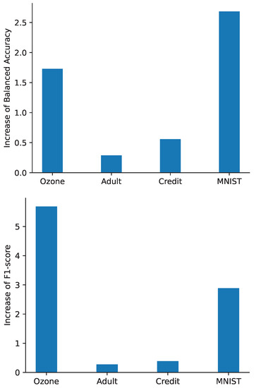
Figure 1.
The mean increase in Balanced Accuracy (on the top) and F1-score (on the bottom) for the four datasets among all the different data-transformation techniques.
5.5. Effects on the Convergence
In principle, the BSBS algorithm is used to improve the convergence speed of the neural network. With the addition of the three new variations of the algorithm—(BSBS-R, NBSBS, and NBSBS-R)—it is imperative to examine how these affect the convergence of the model in general. Usually, the convergence speed is measured the number of epochs it takes to reach a certain score in loss (or accuracy) with respect to the trainset. In order to show that, we will plot the training curve of the accuracy over the epochs of the model. Three data transformation methods were selected for this, ROS, SMOTE and Adasyn. We chose these three because they construct a bigger dataset (oversampling), which will better display the comparison of training speeds. Four setups are compared: training without BSBS, a BSBS(0.1), a NBSBS-R(0.1), and, lastly, a NBSBS-R(0.2). In Figure 2, the training curves are displayed. All BSBS methods are converging much faster, and we can see, in the SMOTE graph, in the middle, that NBSBS-R is a little faster than BSBS at the first epochs, which shows that the variants could be able to achieve better speed at certain situations. Overall, it is clear that the convergence boost that BSBS provides does not decrease when using the variants. On the contrary, it can be beneficial sometimes, although this has to be proven with more experiments and is left as future work.
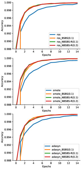
Figure 2.
The training curves of the models for three different data-transformation methods (ROS at the top, SMOTE at the middle, Adasyn at the bottom).
5.6. Comparison with Other Sampling Methods
We tested our algorithm (without any data-transformation applied) with known online sampling algorithms, which have the ability to cope with dataset imbalance. Specifically, online batch selection [21] was selected because it seems to be the first study that incorporates the adaptive batch selection idea. Another sampling technique that was tested was submodular batch selection [29]. The results on the four imbalanced datasets can be found on Table 9 and Table 10 for F1-score and balanced accuracy, respectively. We can see that NBSBS-R performs better than the other methods in both metrics in most of the cases.
Table 9.
F1-score comparison on the generalization with other online sampling methods.
Table 10.
Balanced accuracy comparison on the generalization with other online sampling methods.
Apart from generalization performance, the computational cost of a method is an important characteristic. Below, Table 11 shows the mean training time of the three algorithms that are compared. We can see that our approach is the fastest among the three and in some datasets it finishes training in half the time of the rest. This is being attributed to the fact that the loss that categorizes samples as easy or difficult is an approximation instead of the actual batch loss.
Table 11.
Comparison of mean training times for each dataset.
6. Conclusions
To summarize, this work tackles the problem of imbalanced datasets. These types of datasets are common in real world applications. The objective is to develop methods and algorithms in order to train neural networks that achieve better generalization performance. In this study we presented the sampling algorithm BSBS and proposed two extensions: the first one is through re-enters, while the second one is through added noise in some features of specific samples. The algorithm selects hard examples with certain criteria so that it boosts the learning ability of the network while learning the minority samples adequately.
Through the experimental evaluation, we demonstrated that the proposed algorithm NBSBS-R performs better than the original in four datasets. A variety of data-transformation techniques were tested, and it was shown that our algorithm improved their performance when used in combination. Across all four datasets, the improvement was from up to in some cases regarding balanced accuracy and F1-score. It was also shown that the best setup is, usually, a hybrid method of using a data transformation method (such as SMOTE, RUS, ROS, SMOTETomek, or ENN) alongside NBSBS-R. A comparison was also made with other online sampling methods that showed that NBSBS-R achieves higher F1-score and balanced accuracy. Finally, it was shown that the hybrid method does not suffer any drawbacks regarding the convergence speed, which the original algorithm strives to achieve.
For future work, it would be interesting to incorporate to the main algorithm an adaptive batch size selection. Then, the model can also choose the number of selected samples per batch during the training process along with which samples to include. This can be very beneficial in both performance and computational efficiency. Small batches may lead to better generalization, while bigger ones can accelerate the training time. Other future directions can be the reduction of the memory needed for NBSBS-R to store the sample losses. This can lead to reducing the computational cost and the training time of the algorithm.
Author Contributions
Conceptualization, G.I.; methodology, G.I., A.S. and G.A.; software, G.I.; validation, G.I.; formal analysis, G.A.; resources, G.A.; writing—original draft preparation, G.I.; writing—review and editing, A.S. and G.A.; visualization, G.I.; supervision, A.S.; project administration, A.S. All authors have read and agreed to the published version of the manuscript.
Funding
This research received no external funding.
Data Availability Statement
Code available at https://github.com/geoioannou/NBSBS-R, accessed on 10 January 2023.
Conflicts of Interest
The authors declare no conflict of interest.
Abbreviations
The following abbreviations are used in this manuscript:
| ROS | Random Oversampling |
| RUS | Random Undersampling |
| k-NN | K-Nearest Neighbors |
| SMOTE | Synthetic Minority Oversampling Technique |
| ENN | Edited Nearest Neighbors |
| OCC | One-Class Classification |
| SVDD | Support Vector Data Description |
| SVM | Support Vector Machines |
| OS | Online Sampling |
| SGD | Stochastic Gradient Descent |
| BSBS | Batch Selection with Biased Sampling |
| BL | Batch Loss |
| LL | Low Loss (set) |
| HL | High Loss (set) |
| EMA | Expontential Moving Average |
| NBSBS-R | Noisy BSBS with Re-enters |
References
- Japkowicz, N.; Stephen, S. The class imbalance problem: A systematic study. Intell. Data Anal. 2002, 6, 429–449. [Google Scholar] [CrossRef]
- Guo, X.; Yin, Y.; Dong, C.; Yang, G.; Zhou, G. On the Class Imbalance Problem. In Proceedings of the 2008 Fourth International Conference on Natural Computation, Jinan, China, 18–20 October 2008; Volume 4, pp. 192–201. [Google Scholar] [CrossRef]
- Ioannou, G.; Tagaris, T.; Stafylopatis, A. Improving the Convergence Speed of Deep Neural Networks with Biased Sampling. In Proceedings of the 3rd International Conference on Advances in Artificial Intelligence, ICAAI 2019, Istanbul, Turkey, 26–28 October 2019; pp. 35–41. [Google Scholar] [CrossRef]
- Chawla, N.V.; Bowyer, K.W.; Hall, L.O.; Kegelmeyer, W.P. SMOTE: Synthetic Minority over-Sampling Technique. J. Artif. Int. Res. 2002, 16, 321–357. [Google Scholar] [CrossRef]
- Fix, E.; Hodges, J.L. Discriminatory Analysis. Nonparametric Discrimination: Consistency Properties. Int. Stat. Rev./Rev. Int. Stat. 1989, 57, 238–247. [Google Scholar] [CrossRef]
- Han, H.; Wang, W.; Mao, B. Borderline-SMOTE: A New Over-Sampling Method in Imbalanced Data Sets Learning. In Advances in Intelligent Computing, Proceedings of the International Conference on Intelligent Computing, ICIC 2005, Hefei, China, 23–26 August 2005, Proceedings, Part I; Huang, D., Zhang, X.S., Huang, G., Eds.; Lecture Notes in Computer Science; Springer: Berlin/Heidelberg, Germany, 2005; Volume 3644, pp. 878–887. [Google Scholar] [CrossRef]
- Last, F.; Douzas, G.; Bação, F. Oversampling for Imbalanced Learning Based on K-Means and SMOTE. arXiv 2017, arXiv:1711.00837. [Google Scholar]
- He, H.; Bai, Y.; Garcia, E.A.; Li, S. ADASYN: Adaptive synthetic sampling approach for imbalanced learning. In Proceedings of the 2008 IEEE International Joint Conference on Neural Networks (IEEE World Congress on Computational Intelligence), Hong Kong, China, 1–6 June 2008; pp. 1322–1328. [Google Scholar]
- Drummond, C.; Holte, R. C4.5, Class Imbalance, and Cost Sensitivity: Why Under-Sampling beats OverSampling. In Proceedings of the ICML’03 Workshop on Learning from Imbalanced Datasets, Washington, DC, USA, 21 August 2003. [Google Scholar]
- Wilson, D.L. Asymptotic Properties of Nearest Neighbor Rules Using Edited Data. IEEE Trans. Syst. Man Cybern. 1972, 2, 408–421. [Google Scholar] [CrossRef]
- Anonymous. Two Modifications of CNN. IEEE Trans. Syst. Man Cybern. 1976, SMC-6, 769–772. [Google Scholar] [CrossRef]
- Yen, S.J.; Lee, Y.S. Cluster-based under-sampling approaches for imbalanced data distributions. Expert Syst. Appl. 2009, 36, 5718–5727. [Google Scholar] [CrossRef]
- Batista, G.E.; Bazzan, A.L.; Monard, M.C. Balancing Training Data for Automated Annotation of Keywords: A Case Study. In Proceedings of the II Brazilian Workshop on Bioinformatics, Macaé, RJ, Brazil, 3–5 December 2003; pp. 10–18. [Google Scholar]
- Batista, G.E.A.P.A.; Prati, R.C.; Monard, M.C. A study of the behavior of several methods for balancing machine learning training data. SIGKDD Explor. 2004, 6, 20–29. [Google Scholar] [CrossRef]
- Shamsudin, H.; Yusof, U.K.; Jayalakshmi, A.; Akmal Khalid, M.N. Combining oversampling and undersampling techniques for imbalanced classification: A comparative study using credit card fraudulent transaction dataset. In Proceedings of the 2020 IEEE 16th International Conference on Control Automation (ICCA), Singapore, 9–11 October 2020; pp. 803–808. [Google Scholar] [CrossRef]
- Elkan, C. The Foundations of Cost-Sensitive Learning. In Proceedings of the Seventeenth International Joint Conference on Artificial Intelligence, IJCAI 2001, Seattle, WA, USA, 4–10 August 2001; pp. 973–978. [Google Scholar]
- Kukar, M.; Kononenko, I. Cost-Sensitive Learning with Neural Networks. In Proceedings of the 13th European Conference on Artificial Intelligence, Brighton, UK, 23–28 August 1998; pp. 445–449. [Google Scholar]
- Bengio, Y.; Louradour, J.; Collobert, R.; Weston, J. Curriculum learning. In Proceedings of the 26th Annual International Conference on Machine Learning, ICML 2009, Montreal, QC, Canada, 14–18 June 2009; Danyluk, A.P., Bottou, L., Littman, M.L., Eds.; ACM International Conference Proceeding Series. ACM: Boston, MA, USA, 2009; Volume 382, pp. 41–48. [Google Scholar] [CrossRef]
- Graves, A.; Bellemare, M.G.; Menick, J.; Munos, R.; Kavukcuoglu, K. Automated Curriculum Learning for Neural Networks. In Proceedings of the 34th International Conference on Machine Learning, ICML 2017, Sydney, NSW, Australia, 6–11 August 2017; Volume 70, pp. 1311–1320. [Google Scholar]
- Shrivastava, A.; Gupta, A.; Girshick, R.B. Training Region-Based Object Detectors with Online Hard Example Mining. In Proceedings of the 2016 IEEE Conference on Computer Vision and Pattern Recognition, CVPR 2016, Las Vegas, NV, USA, 27–30 June 2016; pp. 761–769. [Google Scholar] [CrossRef]
- Loshchilov, I.; Hutter, F. Online Batch Selection for Faster Training of Neural Networks. arXiv 2015, arXiv:1511.06343. [Google Scholar]
- Katharopoulos, A.; Fleuret, F. Not All Samples Are Created Equal: Deep Learning with Importance Sampling. In Proceedings of the 35th International Conference on Machine Learning, ICML 2018, Stockholmsmässan, Stockholm, Sweden, 10–15 July 2018; pp. 2530–2539. [Google Scholar]
- Bouchard, G.; Trouillon, T.; Perez, J.; Gaidon, A. Accelerating Stochastic Gradient Descent via Online Learning to Sample. arXiv 2015, arXiv:1506.09016. [Google Scholar]
- Zhao, P.; Zhang, T. Stochastic Optimization with Importance Sampling. arXiv 2014, arXiv:1401.2753. [Google Scholar]
- Bengio, Y.; Senecal, J. Adaptive Importance Sampling to Accelerate Training of a Neural Probabilistic Language Model. IEEE Trans. Neural Netw. 2008, 19, 713–722. [Google Scholar] [CrossRef] [PubMed]
- Alain, G.; Lamb, A.; Sankar, C.; Courville, A.C.; Bengio, Y. Variance Reduction in SGD by Distributed Importance Sampling. arXiv 2015, arXiv:1511.06481. [Google Scholar]
- Chang, H.; Learned-Miller, E.G.; McCallum, A. Active Bias: Training More Accurate Neural Networks by Emphasizing High Variance Samples. In Proceedings of the Advances in Neural Information Processing Systems 30: Annual Conference on Neural Information Processing Systems 2017, Long Beach, CA, USA, 4–9 December 2017; pp. 1002–1012. [Google Scholar]
- Roh, Y.; Lee, K.; Whang, S.E.; Suh, C. FairBatch: Batch Selection for Model Fairness. In Proceedings of the 9th International Conference on Learning Representations, ICLR 2021, Virtual Event, 3–7 May 2021. [Google Scholar]
- Joseph, K.J.; Vamshi Teja, R.; Singh, K.; Balasubramanian, V.N. Submodular Batch Selection for Training Deep Neural Networks. In Proceedings of the Twenty-Eighth International Joint Conference on Artificial Intelligence, IJCAI 2019, Macao, China, 10–16 August 2019; pp. 2677–2683. [Google Scholar] [CrossRef]
- Saini, M.; Susan, S. Deep transfer with minority data augmentation for imbalanced breast cancer dataset. Appl. Soft Comput. 2020, 97, 106759. [Google Scholar] [CrossRef]
- Shi, Y.; Valizadehaslani, T.; Wang, J.; Ren, P.; Zhang, Y.; Hu, M.; Zhao, L.; Liang, H. Improving Imbalanced Learning by Pre-finetuning with Data Augmentation. Proc. Mach. Learn. Res. 2022, 183, 68–82. [Google Scholar]
- Fan, J.; Sun, C.; Chen, C.; Jiang, X.; Liu, X.; Zhao, X.; Meng, L.; Dai, C.; Chen, W. EEG data augmentation: Towards class imbalance problem in sleep staging tasks. J. Neural Eng. 2020, 17, 056017. [Google Scholar] [CrossRef]
- Nie, Y.; Zamzam, A.S.; Brandt, A. Resampling and data augmentation for short-term PV output prediction based on an imbalanced sky images dataset using convolutional neural networks. Sol. Energy 2021, 224, 341–354. [Google Scholar] [CrossRef]
- Chawla, N.V.; Lazarevic, A.; Hall, L.O.; Bowyer, K.W. SMOTEBoost: Improving Prediction of the Minority Class in Boosting. In Knowledge Discovery in Databases: PKDD 2003, Proceedings of the 7th European Conference on Principles and Practice of Knowledge Discovery in Databases, Cavtat-Dubrovnik, Croatia, 22–26 September 2003, Proceedings; Lavrac, N., Gamberger, D., Blockeel, H., Todorovski, L., Eds.; Lecture Notes in Computer Science; Springer: Berlin/Heidelberg, Germany, 2003; Volume 2838, pp. 107–119. [Google Scholar] [CrossRef]
- Seiffert, C.; Khoshgoftaar, T.M.; Hulse, J.V.; Napolitano, A. RUSBoost: A Hybrid Approach to Alleviating Class Imbalance. IEEE Trans. Syst. Man Cybern. Part A 2010, 40, 185–197. [Google Scholar] [CrossRef]
- Lu, Y.; Cheung, Y.; Tang, Y.Y. Hybrid Sampling with Bagging for Class Imbalance Learning. In Advances in Knowledge Discovery and Data Mining, Proceedings of the 20th Pacific-Asia Conference, PAKDD 2016, Auckland, New Zealand, 19–22 April 2016, Proceedings, Part I; Bailey, J., Khan, L., Washio, T., Dobbie, G., Huang, J.Z., Wang, R., Eds.; Lecture Notes in Computer Science; Springer: Cham, Switzerland, 2016; Volume 9651, pp. 14–26. [Google Scholar] [CrossRef]
- Liu, X.; Wu, J.; Zhou, Z. Exploratory Undersampling for Class-Imbalance Learning. IEEE Trans. Syst. Man Cybern. Part B 2009, 39, 539–550. [Google Scholar] [CrossRef]
- Musser, D.R. Introspective Sorting and Selection Algorithms. Softw. Pract. Exp. 1997, 27, 983–993. [Google Scholar] [CrossRef]
- Krizhevsky, A.; Sutskever, I.; Hinton, G.E. ImageNet classification with deep convolutional neural networks. Commun. ACM 2017, 60, 84–90. [Google Scholar] [CrossRef]
- Shorten, C.; Khoshgoftaar, T.M. A survey on Image Data Augmentation for Deep Learning. J. Big Data 2019, 6, 60. [Google Scholar] [CrossRef]
- Cubuk, E.D.; Zoph, B.; Mané, D.; Vasudevan, V.; Le, Q.V. AutoAugment: Learning Augmentation Strategies From Data. In Proceedings of the IEEE Conference on Computer Vision and Pattern Recognition, CVPR 2019, Long Beach, CA, USA, 16–20 June 2019; pp. 113–123. [Google Scholar] [CrossRef]
- Dua, D.; Graff, C. UCI Machine Learning Repository. 2017. Available online: http://archive.ics.uci (accessed on 10 January 2023).
- LeCun, Y.; Cortes, C. MNIST Handwritten Digit Database. 2010. Available online: http://yann.lecun (accessed on 10 January 2023).
- Kingma, D.P.; Ba, J. Adam: A Method for Stochastic Optimization. In Proceedings of the 3rd International Conference on Learning Representations, ICLR 2015, San Diego, CA, USA, 7–9 May 2015. [Google Scholar]
- Nair, V.; Hinton, G.E. Rectified Linear Units Improve Restricted Boltzmann Machines. In Proceedings of the 27th International Conference on Machine Learning (ICML-10), Haifa, Israel, 21–24 June 2010; pp. 807–814. [Google Scholar]
- Buda, M.; Maki, A.; Mazurowski, M.A. A systematic study of the class imbalance problem in convolutional neural networks. Neural Netw. 2018, 106, 249–259. [Google Scholar] [CrossRef] [PubMed]
Disclaimer/Publisher’s Note: The statements, opinions and data contained in all publications are solely those of the individual author(s) and contributor(s) and not of MDPI and/or the editor(s). MDPI and/or the editor(s) disclaim responsibility for any injury to people or property resulting from any ideas, methods, instructions or products referred to in the content. |
© 2023 by the authors. Licensee MDPI, Basel, Switzerland. This article is an open access article distributed under the terms and conditions of the Creative Commons Attribution (CC BY) license (https://creativecommons.org/licenses/by/4.0/).