An Improved Bi-LSTM-Based Missing Value Imputation Approach for Pregnancy Examination Data

Abstract

In recent years, the development of computer technology has promoted the informatization and intelligentization of hospital management systems and thus produced a large amount of medical data. These medical data are valuable resources for research. We can obtain inducers and unknown symptoms that can help discover diseases and make earlier diagnoses. Hypertensive disorder in pregnancy (HDP) is a common obstetric complication in pregnant women, which has severe adverse effects on the life safety of pregnant women and fetuses. However, the early and mid-term symptoms of HDP are not obvious, and there is no effective solution for it except for terminating the pregnancy. Therefore, detecting and preventing HDP is of great importance. This study aims at the preprocessing of pregnancy examination data, which serves as a part of HDP prediction. We found that the problem of missing data has a large impact on HDP prediction. Unlike general data, pregnancy examination data have high dimension and a high missing rate, are in a time series, and often have many non-linear relations. Current methods are not able to process the data effectively. To this end, we propose an improved bi-LSTM-based missing value imputation approach. It combines traditional machine learning and bidirectional LSTM to deal with missing data of pregnancy examination data. Our missing value imputation method obtains a good effect and improves the accuracy of the later prediction of HDP using examination data.

1. Introduction

1.1. Background

Hypertensive disorder in pregnancy (HDP) is a common kind of obstetric complication that severely threatens the life safety of pregnant women [1,2] and has an adverse impact on the growth and development of the fetus. Hence, it is of great significance to discover and cure HDP in advance. Every pregnant woman will have multiple pregnancy examinations during pregnancy, producing examination data capable of reflecting the dynamic changes of health indicators of pregnant women during pregnancy. A huge number of current prediction models make predictions on the basis of multi-source data [3,4], especially for pregnancy examination data [5,6,7]. However, the pregnancy examination data in the real world always contain different kinds of problems. One of the most common issues is missing data. It exists in almost all kinds of data sets, and the size of the missing data can significantly affect the research outcomes. As more and more studies on HDP are turning into data-driven analysis, the missing data problem is becoming more and more critical in this domain.

1.2. Related Work

Nowadays, several scholars have realized the severity of the missing data problem and explored many approaches to reduce the negative effects of missing data. There are several methods now to process missing data. For instance, the most common method, mean filling, uses the mean value of the sample and prior value filling to fill the missing values with the support of medical experts. In addition, there exist some filling methods that have advantages in effect and applicable scenes. For instance, regression filling [8] develops a regression model on the basis of the relationship between the data of each indicator and the pregnancy week to make interpolations to fill the data. KNN (K-nearest neighbors) [9] filling selects K samples that are most similar to the sample to be filled based on a specific kind of similarity measurement algorithm and fills the data with the weighted mean of the full data of the K samples. The matrix completion algorithm [10] decomposes the original data into two low-rank matrices and then uses the gradient descent method to obtain an approximate value to fill missing data.

Although classical methods of statistics, such as interpolation-like techniques, can be used to approximate the missing data in a time series, the recent developments in deep learning (DL) have given impetus to innovative and much more accurate forecasting techniques. Some researchers use a combination of LSTM and transfer learning to fill in missing data values for water quality, air quality, and energy [11,12,13]. Zhou et al. proposed LSTM-based missing data reconstruction for time-series Landsat images [14]. Sowmya et al. combined LSTM with different activation functions to impute the missing data of a diabetic, breast cancer, and wine quality data set [15]. Kostas Tzoumpas et al. combined a CNN and bi-LSTM to fill the missing data of a sensor [16].

1.3. Contributions

All of the above research results are worthy of study. Pregnancy examination data is of high dimension, has a high missing data rate, is in a time series, and often has many non-linear relations, but the above research work has not enabled a richer and more complete extraction of pregnancy examination data in the data pre-processing stage, which in turn has led to poor results regarding missing value filling.

Therefore, we propose an improved bi-LSTM-based missing value imputation approach for pregnancy examination data. The combined model uses the random forest (RF) model principal component analysis (PCA) and undersampling algorithm in the data preprocessing stage, which can analyze the relationships of the features, balance the dataset and filter out abnormal data. Then, bi-LSTM fills the processed data and significantly improves the already good results from other models. This model, compared with the traditional LSTM model, has forward and backward factors to jointly determine the results of filling missing data, which makes the accuracy of filling missing data effectively improved.

2. Materials and Methods

2.1. Data

The data used by this paper are provided by the Institute of Science and Technology of the National Health Commission of PRC, which is the pregnancy examination data of a hospital from 2008 to 2018 (10 years in total, desensitized). The data contained examination records of 120,396 pregnant women, 7518 of whom suffer from HDP, accounting for about 6.24%. In addition, our data covered the pregnancy examination data of the whole pregnancy cycle from early to late maternal pregnancy examination records. The whole pregnancy cycle is the pregnancy examination data from the 1st week to the 70th week, which is very beneficial to our prediction research on HDP and other diseases. Each pregnant woman will take several examinations during the pregnancy of 70 weeks, with each examination corresponding to a piece of data. Each examination does not include all the examination items, and in different stages of pregnancy, the possibility of taking an examination is also different. Figure 1 shows the distribution of the numbers of examinations taken during pregnancy:

The data mainly include 4 parts: pregnogram examination data, routine urine data, routine blood data and biochemical D data. The pregnogram examination data contain the results of 10 kinds of pregnancy examinations, including weight, fundal height, diastolic pressure, fetal position, etc.

Table 1. Indicators of pregnogram examination.

Name	Type	Example
Pregnogram_Fetal Position	Text	“Cephalic”/“Unclear”
Pregnogram_Fetal Heart	Integer	140/150
Pregnogram_Urine Protein	Text	“++”
Pregnogram_Diastolic Pressure	Integer	90/100
Pregnogram_Systolic Pressure	Integer	130/126
Pregnogram_Fundal Height	Integer	31/18
Pregnogram_Abdominal Circumference	Integer	103/80
Pregnogram_Weight	Integer	63/71
Pregnogram_Head-pelvic Relationship	Text	“Floating in”/“Unclear”
Pregnogram_Edema	Text	“++”

lists the name and examples of each indicator. Routine blood data, routine urine data and biochemical D data contain the results of 141 examination indicators, such as platelet count, white blood cell and hemoglobin. Table 1 lists each category and indicator of the 3 examinations. Urine protein (++) means that the urine protein is 1.0–2.0g/L, which is higher than the normal range.Edema ++ indicates a severity level of 2 for edema. All examination indicator can be viewed in

Table A1. Indicators of routine blood, routine urine and biochemical D data.

Routine Urine (UR)	Biochemical D	Routine Blood
UR_White Blood Cell(centrifuged)	Biochemical D_Calcium	Blood Routine_Lymphocyte Percentage
UR_Red Blood Cell(centrifuged)	Biochemical D_Globulin	Blood Routine_Eosinophil Absolute Value
UR_Epithelial Cell(centrifuged)	Biochemical D_Albumin: Globulin	Blood Routine_Platlet Count
UR_Average RBC Hemoglobin Amount	Biochemical D_Total Bilirubin	Blood Routine_RBC Distribution Width
UR_Average Platelet Volume	Biochemical D_Alanine Aminotransferase	Blood Routine_Monocyte Percentage
UR_Fungus	Biochemical D_Iron	Blood Routine_Red Blood Cell
UR_Granular Cast	Biochemical D_Direct Bilirubin	Blood Routine_Eosinophil Percentage
UR_Mucus Strand	Biochemical D_Total Bile Acid	Blood Routine_Monocyte Absolute Value
UR_Abnormal RBC	Biochemical D_Phosphorus	Blood Routine_ Average RBC Hemoglobin Amount
UR_Red Blood Cell	Biochemical D_Aspartate Aminotransferase	Blood Routine_White Blood Cell
UR_Hyaline Cast	Biochemical D_Total Protein	Blood Routine_Basophil Percentage
UR_Urate Crystal	Biochemical D_Glutamic-pyruvic Aminotransferase	Blood Routine_Average RBC Volume
UR_Sulfa Crystal	Biochemical D_Glutamic-pyruvic:Glutamic-oxalacetic	Blood Routine_RBC Distribution Width-SD
UR_Crystal	Biochemical D_Glutamic-oxalacetic Aminotransferase	Blood Routine_Large Platelet Ratio
UR_Epithelial Cell	Biochemical D_Indirect Bilirubin	Blood Routine_Average RBC Hemoglobin Concentration
UR_RBC Cast	Biochemical D_Total Cholesterol	RBC Distribution Width-CV
UR_Normal RBC	Biochemical D_Lactic Dehydrogenase	Glycosylated Hemoglobin
UR_Phosphate Crystal	Biochemical D_Kalium	Blood Routine_Large Platelet Count
UR_Pyocyte	Biochemical D_Carbon Dioxide Concentration	Blood Routine_Urobilinogen
UR_Trichomonad	Biochemical D_Triglyceride	Blood Routine_PH
UR_Inorganic Salt Crystal	Biochemical D_Sodium	Blood Routine_Specific Gravity
UR_WBC Cast	Biochemical D_Creatine Kinase	Blood Routine_Irregular Antibody Screening(3 cells)
UR_Cast	Biochemical D_Creatinine	Blood Routine_Fibrinogen
UR_Waxy Cast	Biochemical D_Uric Acid	Blood Routine_Thrombin Time
UR_Oxalate Crystal	Biochemical D_Chlorine	Blood Routine_Prothrombin Time
UR_Average RBC Volume	Biochemical D_$\gamma$-glutamyl Transpeptidase	Blood Routine_Activated Partial Thromboplastin Time
UR_Progesterone	Biochemical D_Alkaline Phosphatase	Blood Routine_PT International Standardized Ratio
UR_RBC Distribution Width-SD	Biochemical D_Magnesium	Blood Routine_Sugar Shaker
UR_Hemoglobin	Biochemical D_Aspartate:Alanine	Blood Routine_Platelet Distribution Width
UR_Lymphocyte Absolute Value	Biochemical D_Creatinine(enzymic method)	Blood Routine_Hematokrit
UR_Neutrophil Percentage	Biochemical D_Serum Phosphorus	Blood Routine_Basophil Absolute Value
UR_Hematokrit	Biochemical D_Glycated Albumin Ratio	Blood Routine_Average Platelet Volume
UR_Lymphocyte Percentage	Biochemical D_PH	Blood Routine_Lymphocyte Absolute Value
UR_Average RBC hemoglobin Concentration	Biochemical D_Specific Gravity
UR_Intermediate Cell Percentage	Biochemical D_Serum Thyrotropin
UR_Intermediate Cell Absolute Value	Biochemical D_Low Density Lipoprotein Cholesterin
UR_Large Platelet Ratio	Biochemical D_High Density Lipoprotein Cholesterin
UR_Platelet Count	Biochemical D_Serum Free T4
UR_Platelet Distribution Width	Biochemical D_Thyroid Peroxidase Antibody
UR_Neutrophil Absolute Value	Biochemical D_Creatine Kinase Isoenzyme
	Biochemical D_Lipoprotein(a)
	Biochemical D_Apolipoprotein B
	Biochemical D_Apolipoprotein A

in Appendix A.

2.2. Methods

We propose a method that combines traditional machine learning and bidirectional LSTM to deal with the missing data of pregnancy examination data. First, we use traditional machine learning processing methods to remove redundant or unrelated feature data, analyze relationships among the features, and select important features. Then, we use filling methods to fill missing values. After trying different methods, this paper finally selects the bidirectional LSTM (long short-term memory) method to fill a large number of missing data to optimize the dataset. LSTM and its related variants perform very well in many other experiments [17] and in ours. The data processing flow path is shown in Figure 2.

2.3. Traditional Machine Learning

2.3.1. Relationship Analysis of the Features

The examination data in this paper are too large and complicated. After removing redundant data, we used the random forest [18] method to analyze relationships among the features.

The random forest (RF) model, developed on the basis of the decision regression tree model, builds multiple classification trees by the bootstrap method. Then, it selects data randomly to carry out training on each classification tree. Features selected for different classification trees are also chosen at random. Finally, we compared the importance of different features based on the training effect of each classification tree.

Table 2. Top 10 features of importance.

Feature	Relation Degree
Pregnogram_Weight	0.179742
Pregnogram_Diastolic Pressure	0.164976
Pregnogram_Abdominal Circumference	0.139653
Pregnogram_Systolic Pressure	0.138667
Pregnogram_Fundal Height	0.110129
Pregnogram_Fetal Position	0.042483
Pregnogram_Head-pelvic relationship	0.031845
Blood Routine_Platelet Count	0.013081
Blood Routine_Lymphocyte Percentage	0.011491
Blood Routine_White Blood Cell	0.010346

and

Table 3. Bottom 10 features of importance.

Feature	Relation Degree
Biochemical D_Total Protein	0.002450
Biochemical D_Total Bilirubin	0.002394
Biochemical D_Phosphorus	0.002390
Biochemical D_Calcium	0.002237
Biochemical D_Alanine Aminotransferase	0.002205
Biochemical D_Aspartate Aminotransferase	0.002165
Biochemical D_Alobulin	0.001950
Biochemical D_Albumin: Globulin	0.001868
Blood Routine_Basophil Absolute Value	0.001654
Pregnogram_Urine Protein	0.001415

show the top 10 and bottom 10 in terms of importance. It is easy to find that information related to pregnogram data is much more important than information related to biochemical D data, which lays the foundation of our later strategy to fill in missing values and work to reduce the dimension of the data.

2.3.2. Outlier Detection

Outliers are abnormal data that fall outside the cluster. Many fields in medical datasets are manually input, so input errors occur easily. For example, some decimals may be ignored, causing the value to increase 100 times, which obviously leads to abnormal data and results in difficulty in data analysis. This kind of abnormal data will affect the performance of our algorithm if we do not handle it. The concrete method to detect outliers is described as follows.

Detection based on distance measurement [19]: First, we define the distance between samples and then set a threshold distance. Outliers are defined as data points that are far from the others. This method has the advantage of simplicity, which requires low computation and storage costs, but the threshold value is hard to set, and its computation complexity is too big, which is unacceptable for big datasets.

Detection based on clustering algorithms [20]: A clustering model is built, and outliers are defined as data points that are far from all clusters or do not belong to any cluster significantly. This method has an advantage in that there are clustering algorithms that have been developed already, but the method is too sensitive to the selection of the number of clusters.

Detection based on density [21]: The local density of outliers is significantly lower than for neighboring points. The score of an outlier of a sample is the inverse of the density of the area the sample is in. Different definitions of density correspond to different detection methods.

Detection based on statistical methods: A statistical distribution method is built, and outliers are defined as data points with low possibilities. This method has the advantage of the solid foundation of statistics, but it is necessary to obtain the type of distribution of the dataset first; otherwise, it may cause a heavy-tailed distribution.

As this dataset consists of examination indicators, which have relatively fixed ranges, we selected methods based on statistics. For each indicator, we used Matlab to generate a scatter diagram. As the number of outliers was too small, we detected them with a priori knowledge and manually selected them to fix or propose.

2.3.3. Data Filtering

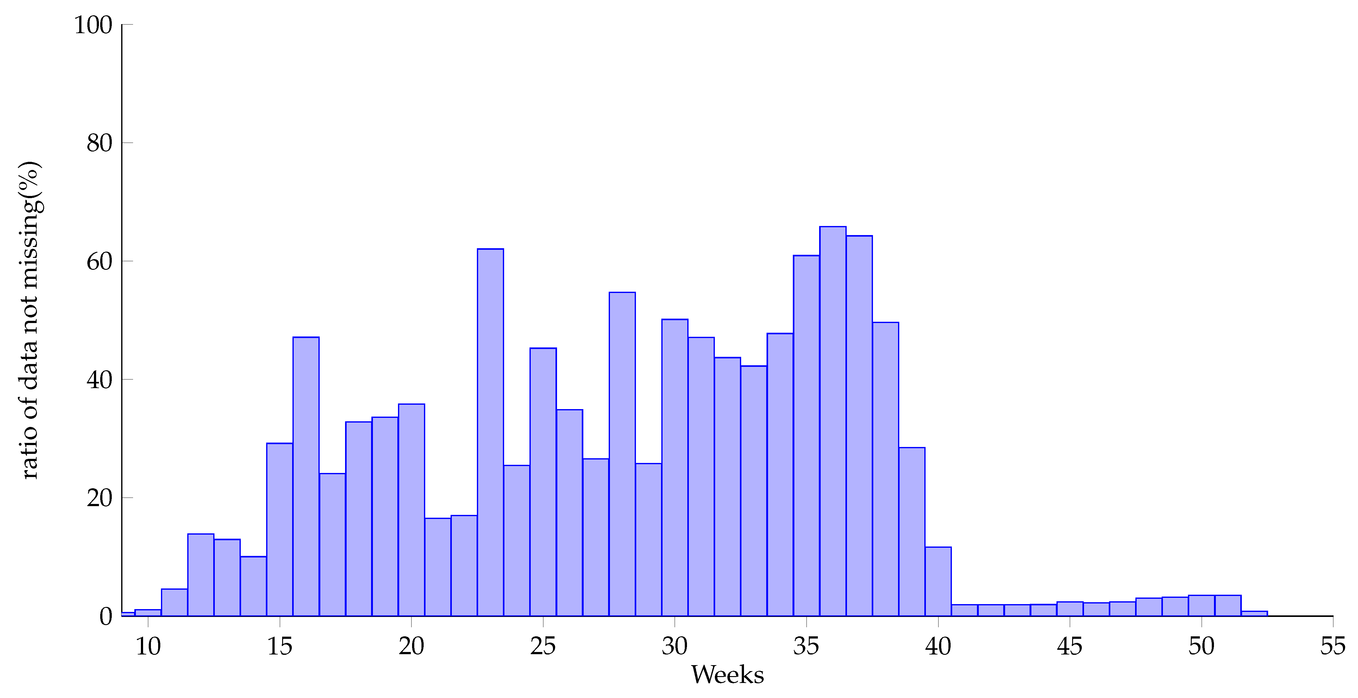
According to the missing mechanism, Rubin [22] divided missing data into 3 categories: completely random missing, random missing and incompletely random missing data. This dataset is of the category of incompletely random missing data. The missing nature of the data depends on the pregnancy week. After analysis, the missing data rate of each pregnancy week is shown in Figure 3. It can be found that data are mainly in the range from week 11 to week 40 (with the ratio of data not missing over 5%), and the later the weeks are, the more pregnancy examination records there are. Therefore, this paper selects data from week 11 to week 40 to be processed and analyzed.

As some pregnant women have relatively few examinations, in the 30 weeks from week 11 to week 40, about 10% of the samples have less than 5 examinations. To improve the quality of the dataset, these data should be removed. However, to utilize the dataset as much as possible, this paper uses the selection method described as follows. We consider the degree of the concentration of the pregnancy weeks of the sample with low examination times. If the pregnancy weeks of the examinations are concentrated in the early or late weeks, the sample is considered to be worthless and removable, but if the weeks are scattered, the sample is considered to have the effect of “supporting” and should be kept. Therefore, this paper calculates the ratio of the range between the pregnancy weeks of each sample and the selected pregnancy week range and selects samples with a ratio greater than 0.8.

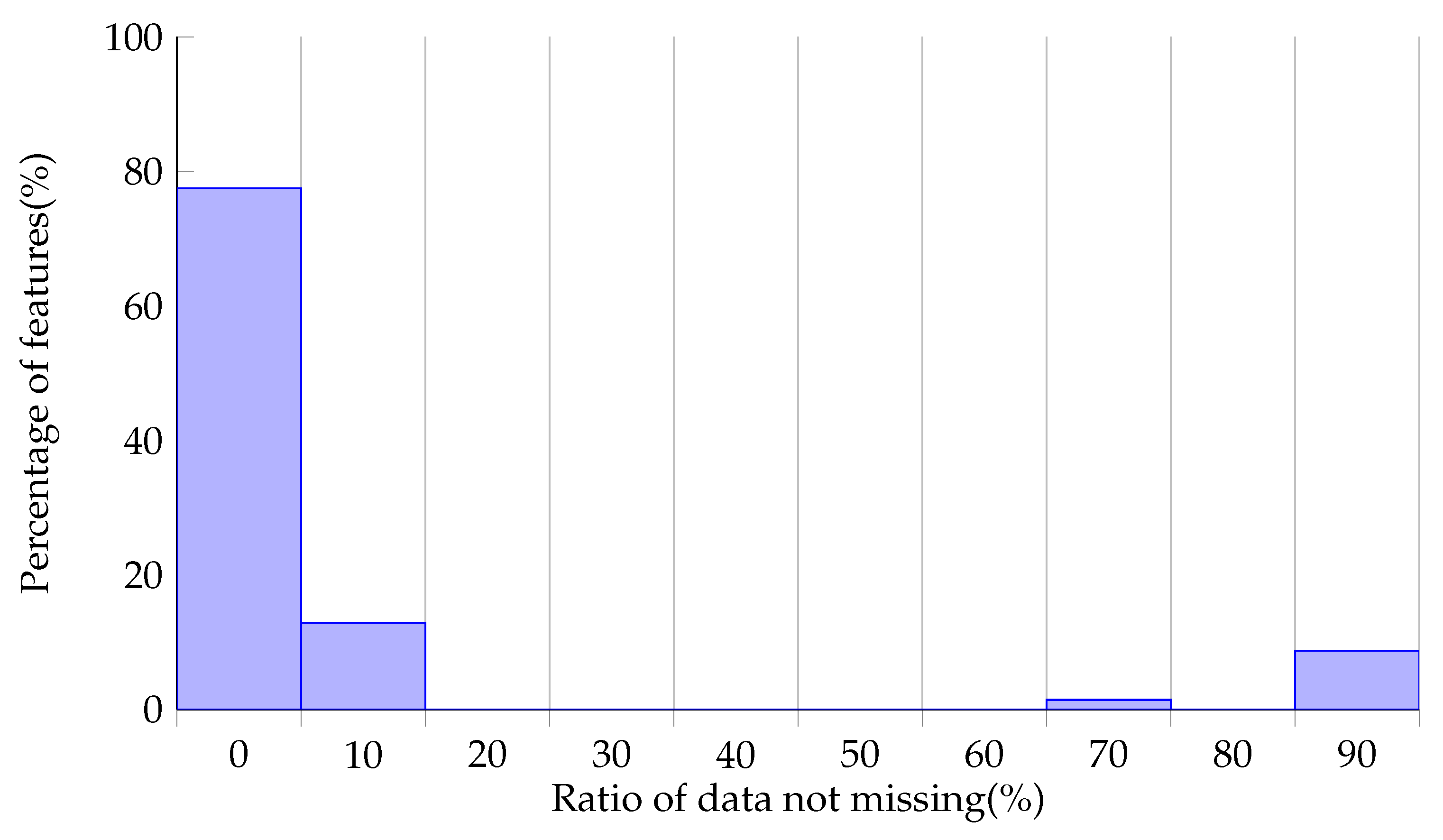
This dataset has a large number of complicated indicators, the total number of which is 200. The missing status on each feature is shown in Figure 4. It is shown that that data of most features are severely missing, with only about 10% left. The data of a small number of features are in a good state. Considering the model’s performance and the difficulty of training, we selected features with a missing rate lower than 30% to build the dataset.

2.3.4. Feature Extraction

In the previous relationship analysis of features, except for a few kinds of information of pregnograms that are highly related with the disease state of pregnant women, the relationship of a large amount of information of biochemical D, routine blood, and routine urine data is relatively scattered, but they contain a lot of health information regarding the pregnant women. Therefore, methods such as the missing rate ratio, low variance filtering, high relation filtering, and even random forest are not suitable for feature extraction in this paper. The reason is that these methods directly remove a large number of irrelevant features in the dimension reduction process, which greatly damages the richness of the dataset of HDP.

On the other hand, the dataset of HDP is large, containing nearly one million data records. Therefore, the efficiency of feature extraction is also an important factor affecting our decision.

Table 4. Comparison of common feature extraction methods.

Common Dimension Reduction Methods	Drawbacks
Missing rate ratio	Removing features directly, harming data richness
Low variance filtering
High relation filtering
Random forest
Reverse feature removal	Consuming too much time
Forward feature construction

is a comparison of common feature extraction methods. Reverse feature removal and forward feature construction both need to pre-train the model to select features. The size of the dataset of HDP greatly limits the speed of the model’s training, causing the feature extraction work to consume too much, so they are also not feasible.

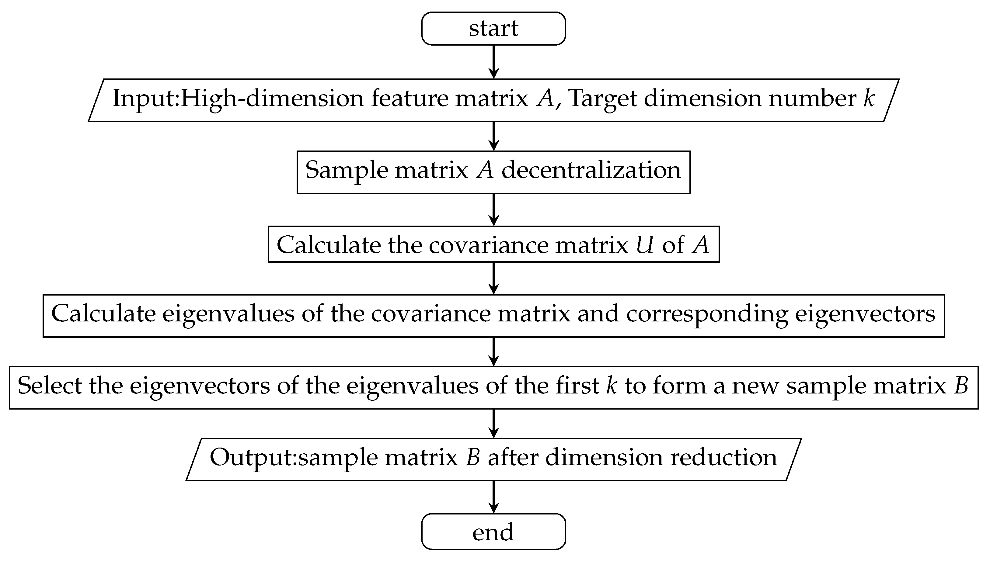
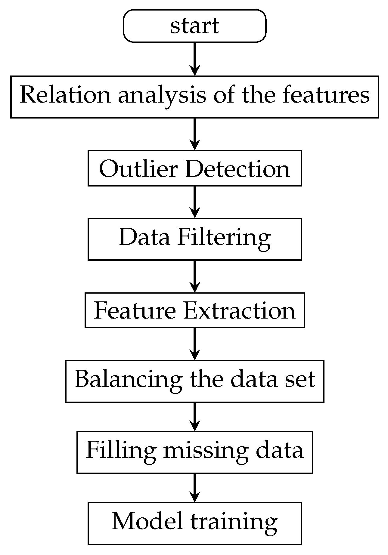
After comprehensive consideration, this paper selected principal component analysis (PCA) for the reduction of the dimensions of the data of the HDP dataset [23,24]. Considering the characteristics of the prediction model of HDP, the dataset of HDP after dimension reduction has 32 feature items. Figure 5 shows the process of feature extraction.

2.3.5. Balancing the Dataset

The positive and negative samples are extremely imbalanced in the original dataset, the proportion of which is about 1:10. If original data are used for training directly, the model will not be able to learn the characteristics of positive samples effectively. There are two common methods to balance a dataset: using an oversampling method, such as SMOTE [25], and undersampling. Oversampling will copy or approximate the samples with a small number to supplement the samples so as to balance the number of positive and negative samples. However, such a method to copy or approximate samples will increase the risk of over-fitting, especially in this case of an extreme imbalance of positive and negative samples. Therefore, this paper used the method of random undersampling of negative samples. Negative samples with a number equal to the positive samples were randomly selected to construct the dataset. This method also reduces the difficulty and cost of training effectively.

2.3.6. Processed Data

Table 5. Changes before and after data processing.

Data	Original Data	Preprocessed Data
Number of examination records	120,396	53,272
Number of features	141	36

shows the changes before and after data preprocessing. After traditional machine learning processing, redundant and useless data were eliminated. We only retained feature data that were highly relevant to the HDP. The following experiments are based on the processed data.

2.4. Strategy to Fill Missing Values—Bi-LSTM

This dataset has severe missing data in the dimensions of time and features, so it is of great significance to discuss the influence of missing data processing on the model’s effect. There are three ways to analyze data with missing values: (1) analyze the data with missing values directly; (2) select methods that are insensitive to missing data for analysis; (3) analyze the missing data after interpolation and filling. Filling missing data has always been a hot topic in various fields. Currently, several effective missing data filling methods have been proposed by experts and scholars. For example, the commonly used mean value interpolation method uses the mean value of sample variables to replace the missing value [26]. Random interpolation, on the basis of the sample distribution, extracts a substitution of missing values with a specific possibility from the population. Regression interpolation uses the linear relationship between auxiliary variables and target variables to predict missing values. Dempster proposed the EM (expectation maximization) algorithm [27] in 1977, which is used to estimate unknown parameters under known variables and can effectively carry out the task of the interpolation of missing data. These methods have high accuracy when filling a small amount of missing data in a static situation but are not satisfactory when processing missing data with a nonlinear relationship, time series characteristics and multiple variables. Recently, with the rapid development of the field of neural networks and the improvement of computing capabilities, neural networks have been widely used in the processing and analysis of missing data, recurrent neural networks (RNN) [28] especially. They are capable of finding long-term time dependences and analyzing time series of variable length, thus playing a very important role in time series analysis.

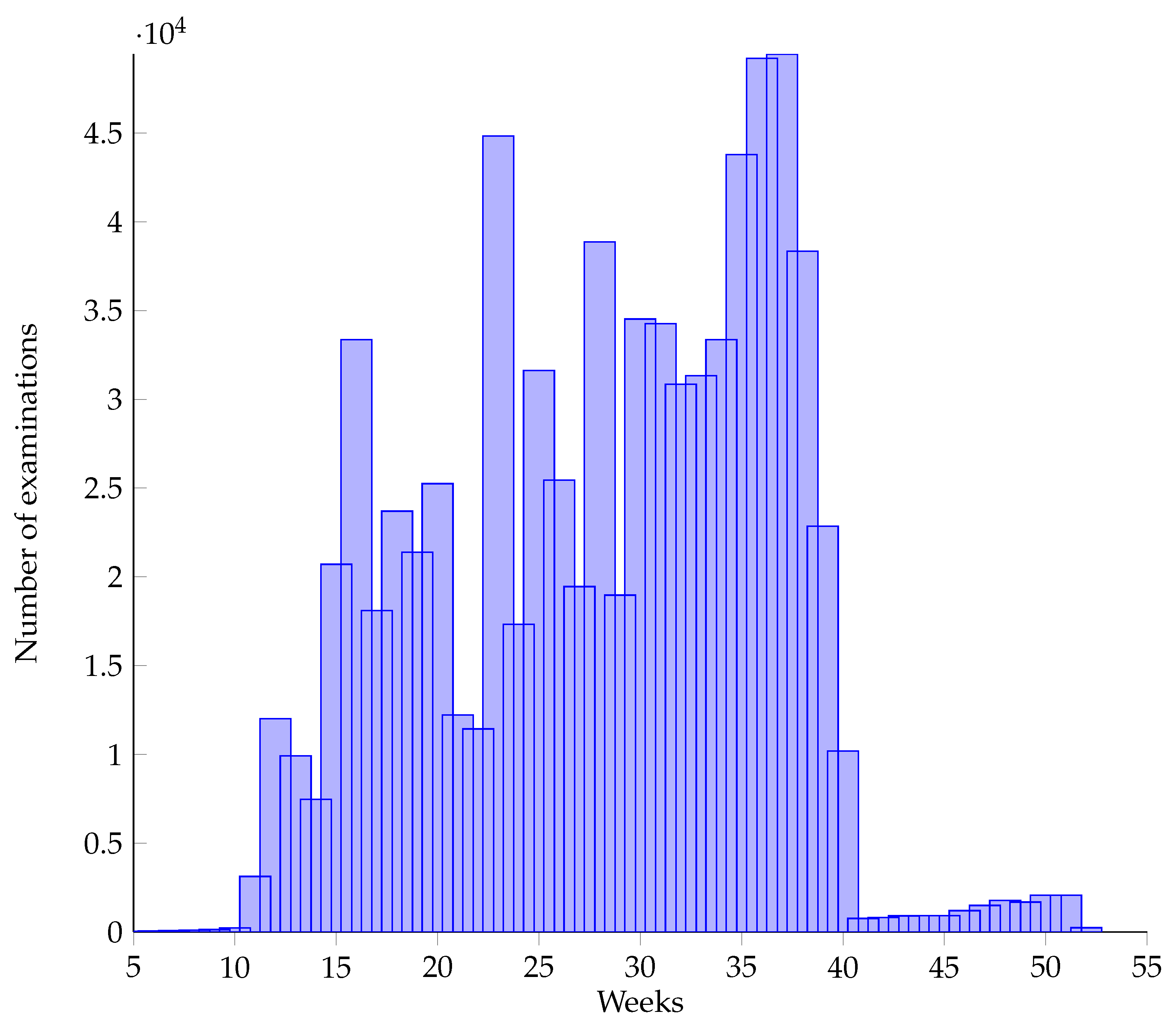
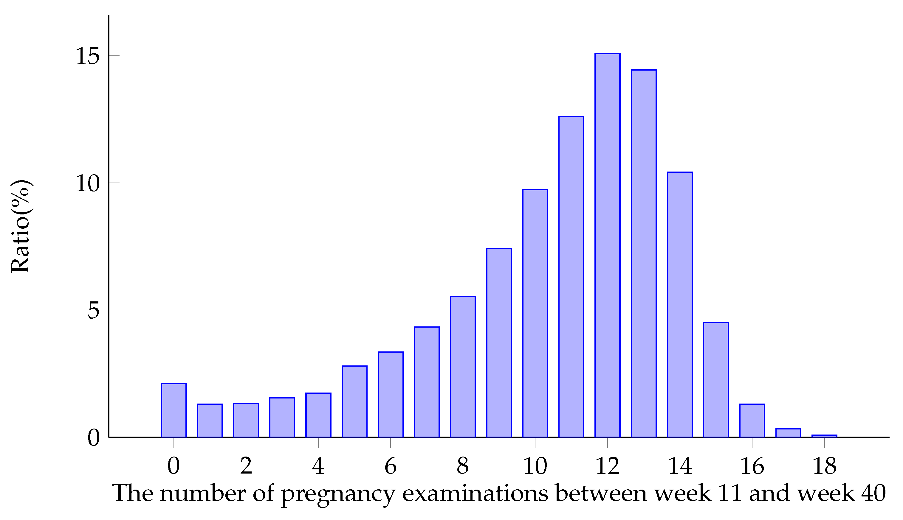
Figure 6 shows the distribution of the number of pregnancy examinations (i.e., the length of time series) between week 11 and week 40. It can be seen from the figure that the length of the series of most samples is about 11 times. In Figure 1, it can be seen that the data are not uniformly distributed at different time points, and most of the data are concentrated in the later weeks.

This paper selected data of a part of time as markers and selected other data as training data. The filling effect was evaluated by the prediction results and symmetric mean absolute percentage error (SMAPE) of markers. Considering the distribution of data at each time point, markers should not be selected randomly in order to prevent losing the data of important time points and severely affecting the results. This paper proposes a method described as follows: let $X=x_1,x_2,\dots ,x_i,\dots ,x_n$ represent the missing state of a series of data:

$$x_i=\left\{\begin{array}{c}1,\mathrm{data}\mathrm{of}\mathrm{time}\mathrm{point}i\mathrm{exists}\hfill \\ 0,\mathrm{data}\mathrm{of}\mathrm{time}\mathrm{point}i\mathrm{are}\mathrm{missing}\hfill \end{array}\right.$$

(1)

For $A=a_1,a_2,\dots ,a_i,\dots ,a_n$,

$$a_i=\frac{{\Sigma }_{k=1}^n{x}_k·{\gamma }^{|k-i|}-x_k}{\Sigma a_i}$$

(2)

$a_i$ represents the “ignorability” of the data of the time point in the series. The less missing data near this value, the more “unimportant” the time point is, and it can be selected from the training set as a marker, where $\gamma$ is the decay rate.

Table 6. Calculation sample of “ignorability” of data in time series.

x	1	0	0	0	1	0	1	1	1	0
$\beta$	0.011	0.085	0.076	0.105	0.062	0.176	0.127	0.142	0.102	0.113

is the result of calculating the missing data state when the sequence length is 10 and the decay rate is 0.5.

For $B=b_1,b_2,\dots ,b_n$,

$$b_i=\frac{\Sigma x_i}{\Sigma b_i}$$

(3)

$b_i$ represents the data storage rate of time point i in the whole data set. The higher it is, the lower the missing data rate of the time point is, and the lower the possibility it needs to be filled is. Thus, for each series, the possibility that each time point is selected to be a marker $p_i=\alpha \ast a_i+\beta \ast b_i$, where $\alpha$ and $\beta$ are the parameters that adds up to 1, which are used to adjust the influence of the two parts of the possibility. We select data of a certain number of time points in each series as markers to construct the data and markers of the training set. According to distribution of the data, the final parameters used in this paper are $\gamma =0.5,\alpha =0.8,\beta =0.2$, and the data at four time points are selected as markers.

In this paper, we compare several methods of filling missing values, including traditional machine learning methods, such as cubic spline interpolation and KNN filling, and deep learning methods, such as the LSTM model and bidirectional LSTM model.

1

Cubic spline interpolation

Cubic spline interpolation (spline interpolation) [29] is a process of obtaining the curve function group by solving the three-moment equations through a series of value points on the curve. First, we select an interval containing missing values of the dataset, construct a cubic interpolation equation to represent the interval, and then conduct interpolation for the missing values according to the equation.

2

KNN filling

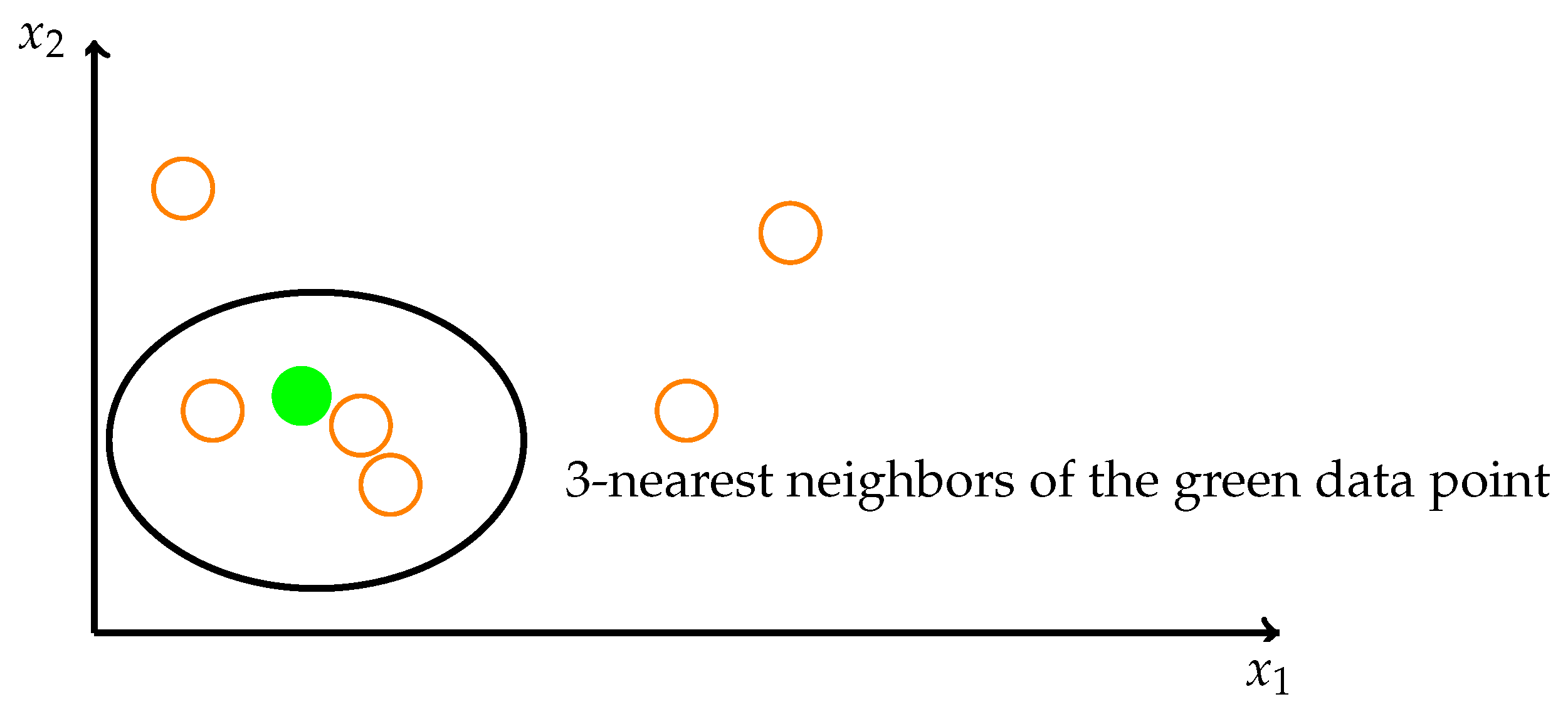
The idea of the KNN method is to identify k spatially similar samples in the dataset. We then use these “k” samples to estimate the value of the missing data points. The missing value of each sample is interpolated using the mean value of the “k” neighborhood found in the data set. In this case, as Figure 7 shows, the missing value is determined by its neighbors. The green point’s neighbors are the orange points in the ellipse. Each pregnant woman’s data are mapped to a vector in a high-dimensional space. To be spatially close means to be physically similar.

3

ST-MVL

ST-MVL is a spatio-temporal multiview-based learning (ST-MVL) method [30] to collectively fill missing readings in a collection of geosensory time series data considering (1) the temporal correlation between readings at different timestamps in the same series and (2) the spatial correlation between different time series. The method combines empirical statistic models, consisting of inverse distance weighting and simple exponential smoothing, with data-driven algorithms, comprised of user-based and item-based collaborative filtering.

4

LSTM Model

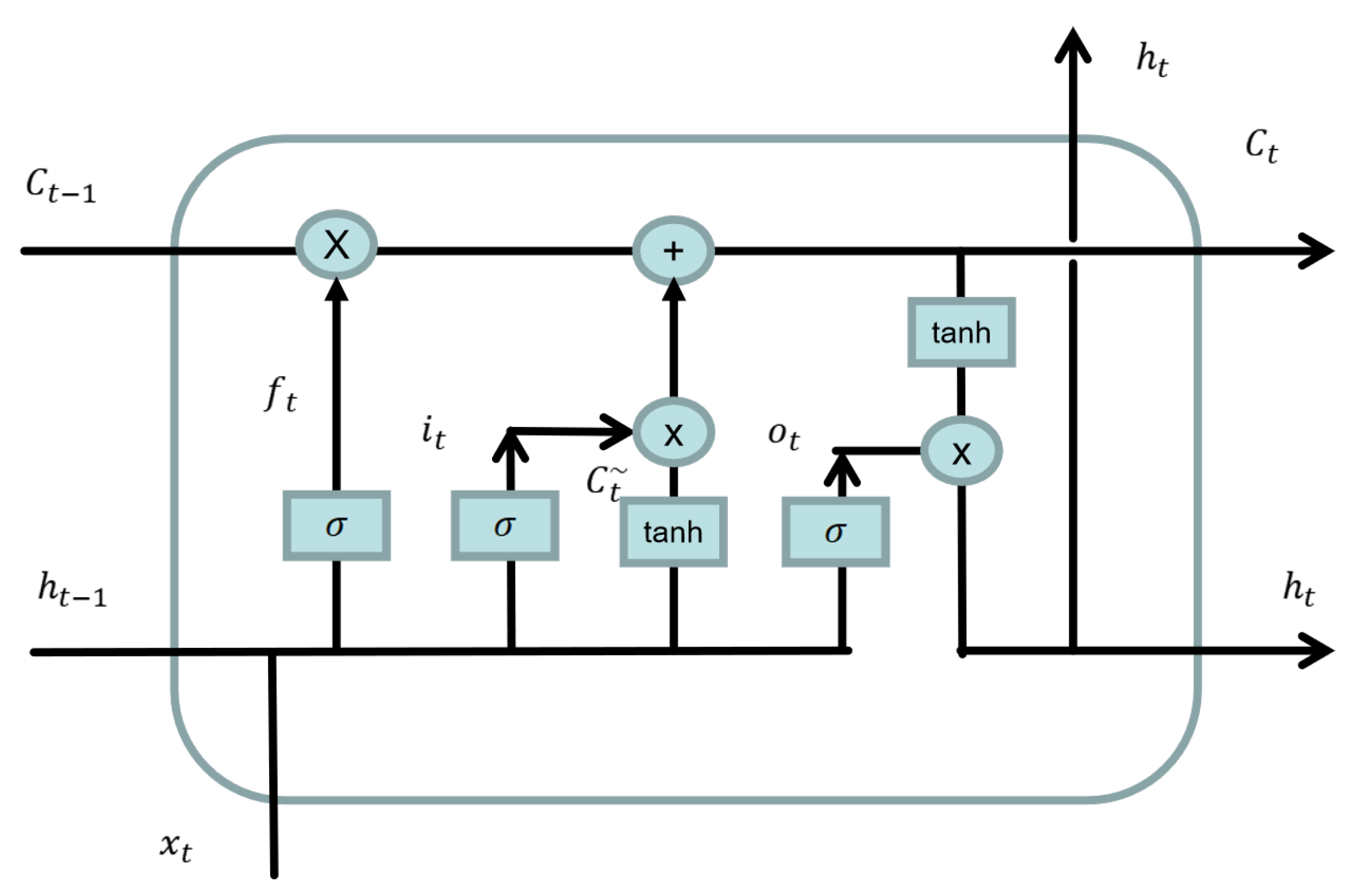
The LSTM model is a special kind of recurrent neural network (RNN), which was first proposed by Hochreiter and Schmidhuber [31] in 1997 and solved the problem of the vanishing gradient and long-term dependence (i.e., the inability to integrate dependencies of a series that are too long) of RNNs. As shown in Figure 8, an LSTM consists of a memory unit c and three gates (an input gate i, output gate o, and forgetting gate f).

The first step of the LSTM is to determine how much of the state of the previous time point $c_{t-1}$ will be retained to the current moment $c_t$. This decision is made by the “forgetting gate”. The forgetting gate uses the output $h_{t-1}$ of the previous neural cell and the input $x_t$ of the current cell to calculate a number between 0 and 1, representing how much data from the previous cell was recorded. Here, 1 indicates complete recording, and 0 indicates complete forgetting. The equation is shown as follows, where $W_f$ is the weight matrix of the forgetting gate, $b_f$ is the bias term of the forgetting gate, and $\sigma$ is the sigmoid activation function:

$$f_t=\sigma (W_f·[h_{t-1},x_t]+b_f)$$

(4)

The second step of LSTM is to determine what information is to be stored in the current unit state, which is divided into two parts. First, an input gate determines which values to update, and then a new candidate vector $C_t^{\sim }$ is created through the tanh layer and added to the state. The current state of the unit is calculated as follows. First, we forget the data that need to be forgotten by multiplying the state of the last time point by $f_t$. Then, we add $i_t\ast C_t^{\sim }$ to obtain the value of the current unit:

$$i_t=\sigma (W_i·[h_{t-1},x_t]+b_i)$$

(5)

$$C_t^{\sim }=tanh(W_c·[h_{t-1},x_t]+b_c)$$

(6)

$$C_t=f_t\ast C_{t-1}+i_t\ast C_t^{\sim }$$

(7)

The third step of the LSTM is to determine the output of the unit. The output is based on the state of previous calculating unit, first through the sigmoid layer to determine which parts of the unit to output, then through tanh to reset the system state (setting the value to between −1 and 1). Then, we multiply it by a sigmoid gate to determine the final output:

$${\sigma }_t=\sigma (W_o·[h_{t-1},x_t]+b_o)$$

(8)

$$h_t=o_t\ast tanh\left(C_t\right)$$

(9)

5

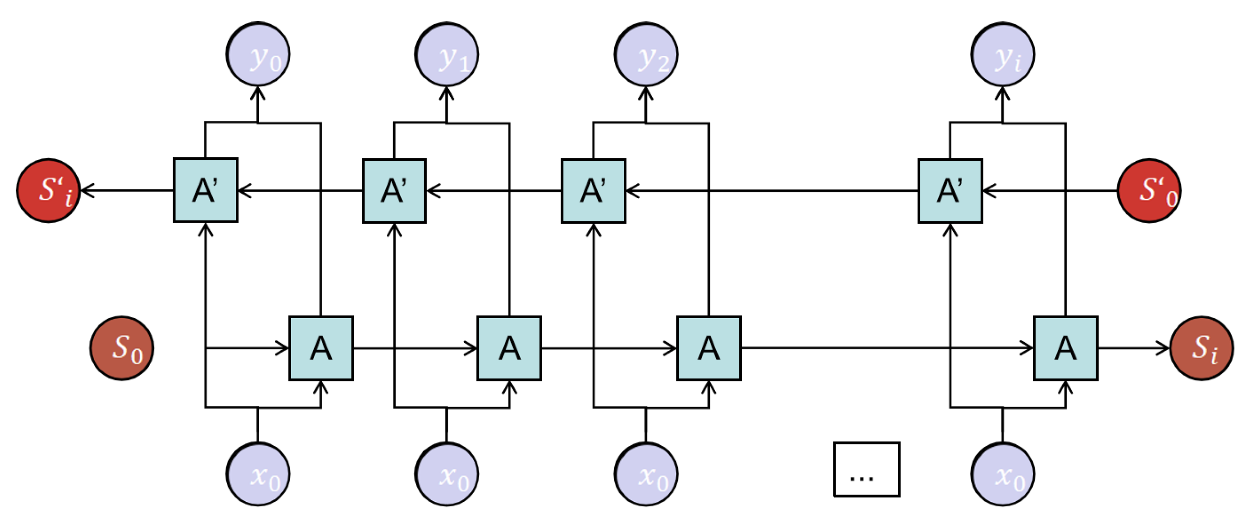
Bidirectional LSTM Model

The bidirectional LSTM model consists of a forward LSTM structure and a reverse LSTM structure, as is shown in Figure 9. They have the same structure and are independent of each other and only accept input of different word orders. The bidirectional LSTM deep learning network has great advantages, a clear structure, a clear output meaning of the middle layer, and it is easier to find optimization methods for it. The bidirectional LSTM model takes the influence of forward and reverse word order of sentences into account, which can better extract the semantic information of sentence structures. In this task, compared with unidirectional LSTM, the effect of filling missing data with bidirectional LSTM is better.

3. Results and Analysis

3.1. LSTM Model Hyperparameters

The hyperparameters of model training are shown in

Table 7. Hyperparameter Settings.

Optimizer	Adam method
Loss function	Cross-entropy and L2 regulation = ${\sum }_{i=1}^N[y_{i}log\widehat{y_i}+(1-y_i)log(1-\widehat{y_i})]+{\lambda \left|\right|w\left|\right|}_2^2$
Parameter initialization	Set value to zero.
Dimension of word vectors	32
Dimension of position vectors	5
Batch	128
Adam learning rate	$1.00\times {10}^{-3}$

.

3.2. Analysis of Experimental Results

In this paper, we propose an improved bi-LSTM-based missing value imputation approach for pregnancy examination data. This model, compared with the traditional LSTM model, has forward and backward factors to jointly determine the results of filling miss data, which makes the accuracy of filling missing data effectively improved. This paper selects the results on the validation set after training on 70% of the preprocessed data as the training set.

Table 8. Comparison of different filling methods.

Filling Methods	Cubic Spline Interpolation	KNN Filling	LSTM Model	ST-MVL	Improved Bidirectional LSTM Model
SMAPE (%)	8.745	6.746	8.796	6.734	6.569

shows the comparison of different filling methods. This paper uses SMAPE to evaluate the missing values. It is shown that the bidirectional LSTM model interpolation method has the best filling effect regarding missing data compared with other methods. The experiment found that ST-MVL is not good for filling data columns with serious missing data, so we used data with a missing rate of less than 50% for ST-MVL experiments.

In addition, the lightgBM disease prediction algorithm [32] was used to compare the training model before and after data filling. As is shown in Figure 10, the blue curve represents the training results using the complete data of pregnancy weeks filled by LSTM, and the orange curve represents the training results using unfilled pregnancy week data. It can be seen that the accuracy of the prediction results after filling is higher. In addition, it can be seen that the prediction accuracy is positively correlated with the number of pregnancy weeks. From the figure above, it can be seen that the model has a good prediction effect at just 25–26 pregnancy weeks, and the AUC of the HDP prediction effect can reach more than 0.75. From 25 weeks on, forecasts continuously improve. Data from week 25 to week 40 are more important to model predictions than data before week 25.

4. Conclusions and Future Work

HDP is a common obstetric complication that severely threatens the life of pregnant women. Therefore, it is of great significance to detect and prevent HDP in advance. However, pregnancy examination data have the characteristics of high dimensions, large amounts, being in a time series and having a high missing rate, so a good data processing method plays an extremely important role in predicting and preventing HDP. This paper first introduces pregnancy examination data in detail and then proposes a series of data processing strategies, including basic data processing methods such as feature relation analysis, data filtering, feature extraction, balancing the dataset, etc. This paper also puts forward a method of missing value filling based on a bidirectional LSTM model and makes a comparison with cubic spline interpolation, KNN filling and an LSTM model, the results of which show that the bidirectional LSTM model achieves good results in filling missing data. Although this paper has made some progress in data processing, especially in filling missing data, there is still much work to be further studied and explored, including the following aspects:

• In data processing, there are still some factors that are not considered, such as region, age, etc.
• The method of filling missing valuesis relatively simple at present, and the future research direction is to combine multiple algorithms to deal with different features.
• At present, the data preprocessing process is basically manual processing, so it can save a lot of time and stamina to standardize the processing process and build ETL (extract-transform-load) tools automatically.
• After prediction, screening proper drug treatment programs [33] is also important for doctors and patients. Building a complete intelligent medical system is very meaningful.
• At present, the amount of research data in the medical field is very large, but these data are often chaotic. The format of diagnostic data in different medical institutions is not uniform, so it is difficult to use it directly for research. Constructing a complete standardized medical research database is of great significance for disease prevention, drug development, and other research.