Article

On the Influence of Data Imbalance on Supervised Gaussian Mixture Models

Department of Economics, Università degli Studi di Perugia, Via A. Pascoli 20, 06123 Perugia, Italy
Algorithms 2023, 16(12), 563; https://doi.org/10.3390/a16120563
Submission received: 7 November 2023 / Revised: 5 December 2023 / Accepted: 5 December 2023 / Published: 11 December 2023
(This article belongs to the Special Issue Algorithms in Data Classification)

Abstract

:
Imbalanced data present a pervasive challenge in many real-world applications of statistical and machine learning, where the instances of one class significantly outnumber those of the other. This paper examines the impact of class imbalance on the performance of Gaussian mixture models in classification tasks and establishes the need for a strategy to reduce the adverse effects of imbalanced data on the accuracy and reliability of classification outcomes. We explore various strategies to address this problem, including cost-sensitive learning, threshold adjustments, and sampling-based techniques. Through extensive experiments on synthetic and real-world datasets, we evaluate the effectiveness of these methods. Our findings emphasize the need for effective mitigation strategies for class imbalance in supervised Gaussian mixtures, offering valuable insights for practitioners and researchers in improving classification outcomes.

1. Introduction

1.1. Motivation

Gaussian mixture models (GMMs) are probabilistic models widely employed in clustering and density estimation tasks which provide a flexible framework for modeling complex data distributions [1,2,3]. These models represent data as a finite mixture of Gaussian distributions with unknown parameters, where the latter are often estimated through the Expectation-Maximization (EM) algorithm [4,5].
In addition to the aforementioned unsupervised tasks, GMMs also find application in classification tasks. Supervised Gaussian mixture models (SGMMs) proved to be effective in this domain due to their ability to represent complex data patterns. However, these models are sensitive to class imbalance, where the number of samples in one or more classes significantly differs from the others, leading to biased parameter estimation, diminished generalization, and reduced accuracy [6,7]. This scenario is especially relevant in domains such as fraud detection, rare event prediction, disease diagnosis, and many other classification and pattern recognition problems. Despite these drawbacks, data imbalance in GMMs has received little attention in the literature [8,9].

1.2. Aim and Organization of the Paper

In this paper, we restrict our attention on evaluating the effect of data imbalance on SGMMs classification accuracy and comparing various strategies to address this challenge. Specifically, we assess techniques such as cost-sensitive learning, probability threshold adjustment, threshold selection through cross-validation, and sampling-based approaches, such as downsampling, oversampling, and SMOTE.
Through a comprehensive set of experiments on diverse datasets, both synthetic and real data examples, we systematically evaluate the performance of GMM classifiers with and without these adjustment strategies. This empirical analysis aims to provide insights into the effectiveness of these methods in handling data imbalance and improving classification outcomes.
The remainder of this paper is organized as follows. Section 2 is devoted to the presentation of probabilistic models for supervised learning in classification with particular focus on Gaussian mixture models, and the corresponding classification rule that can be derived. Performance measures for imbalanced data are discussed in Section 4, including cost-sensitive learning, different threshold adjustments techniques, and sampling-based approaches. Section 5 presents an extensive investigation through simulation studies on synthetic data and empirical analyses using real-world datasets. Lastly, the final section concludes by highlighting the key contributions of this paper.

2. Materials and Methods

2.1. Probabilistic Generative Models for Supervised Learning

In probabilistic classification, a statistical model is employed to predict the class C k (where k = 1 , , K ) for a given observation characterized by a feature vector x i . This model provides a posterior class probability, denoted as Pr ( C k x i ) , for each class, which is subsequently utilized to determine class membership for novel observations.
Certain modeling techniques directly estimate posterior probabilities by constructing a discriminant function η k ( x i ) , that directly maps features x i to each class C k . These are known as discriminative models, with a prominent example being the logistic regression model for binary-class problems.
Alternatively, other approaches aim to model the distribution of both features and classes, either explicitly or implicitly. Posterior probabilities are then derived using Bayes’ theorem. Consequently, through the learning of class-specific densities f ( x i C k ) and the prior class probabilities Pr ( C k ) for each class, the posterior class probabilities can be calculated as:
Pr ( C k x i ) = f ( x i C k ) Pr ( C k ) g = 1 K f ( x i C g ) Pr ( C g ) .
Approaches following this methodology, such as those rooted in finite mixture modeling, are referred to as generative models.
Assume a training dataset D train = { ( x 1 , y 1 ) , , ( x n , y n ) } is available, for which both the feature vectors x i and the true classes y i = { C 1 , , C K } for each observation are known. Classification models are fitted using data from such a training set, ultimately yielding parameter estimates. However, if this same dataset is also employed for tasks like model fine-tuning (such as hyperparameter estimation) and classifier evaluation, it tends to yield an overly optimistic evaluation of performance. This phenomenon is termed overfitting, signifying the potential hazard of tailoring a model too closely to a specific set of data, which may consequently struggle to generalize well to additional data or predict future observations accurately. Given these considerations, it is recommended to carry out model fine-tuning using a validation set, a dedicated dataset typically reserved separately from the original dataset. Alternatively, one can adopt resampling techniques, such as cross-validation, which involve repeatedly partitioning the data into training and validation sets. If enough data are available, a separate subset of the initial dataset could be set aside in advance as a test set for the final evaluation of the classifier.

2.2. Gaussian Mixtures for Classification

Classification models based on Gaussian mixtures make the assumption that the density within each class follows a Gaussian mixture distribution:
f ( x i C k ) = g = 1 G k π g | k N ( x i μ g | k , Σ g | k ) ,
where G k represents the number of components within class k. The  π g | k terms denote the mixing probabilities for class k ( π g | k > 0 and g = 1 G k π g | k = 1 ), and  μ g | k along with Σ g | k stand for the mean vectors and covariance matrices for component g within class C k .
One earlier proposal is the Mixture Discriminant Analysis (MDA) model [10], where it is posited that the number of mixture components is known and equal across classes, with equal full covariance matrix across classes, so Σ g | k = Σ for all g = 1 , , G k and k = 1 , , K in Equation (1).
A much more constrained model is the Eigenvalue Decomposition Discriminant Analysis (EDDA) model [11], which assumes that the density for each class can be characterized by a single Gaussian component, so G k = 1 for all k in Equation (1). Furthermore, in this model, the covariance structure of each class is factorized as:
Σ k = λ k U k Δ k U k .
A list of models obtained from the eigen-decomposition in (2), with associated geometric characteristics, is reported in Table 2.1 of Scrucca et al. [12]. Through this decomposition, several classification models can be derived. When each component shares the same covariance matrix, i.e.,  Σ k = λ U Δ U , the corresponding model is equivalent to the classical Linear Discriminant Analysis (LDA) model. On the other hand, if the component covariance matrices are unrestricted and differ between components, i.e.,  Σ k = λ k U k Δ k U k , EDDA is equivalent to the Quadratic Discriminant Analysis (QDA) model. Naïve-Bayes models can also be obtained by assuming conditional independence of features within each class, so component covariance matrices are all diagonal, eventually with equal values along the main diagonal for the case of equal variances among features.
The broadest model encompassed by Equation (1) framework is the MclustDA model [2], which employs a finite mixture of Gaussian distributions within each class, allowing for flexibility in the number of components and covariance matrices, with the latter parameterized using the eigen-decomposition shown in Equation (2). Specifically, each class may exhibit a distinct Gaussian mixture, and the covariance matrix characteristics can vary across classes. This enables the model to capture a wide range of data distributions and provides a powerful tool for classification tasks that involve complex, heterogeneous datasets.

2.3. Model Selection

MclustDA models, and to a lesser extent EDDA models, offer a versatile approach to classification. As is often the case, the increased flexibility they introduce may lead to an increased risk of overfitting. Therefore, it becomes crucial to apply a model selection criterion that strikes a balance between the goodness of fit and the parsimony of parameterization. The Bayesian information criterion [13] (BIC) is a common tool employed for choosing the “best” model from a set of candidate models. For a given model M it is defined as
BIC M = 2 M ( θ ^ ) ν M log ( n ) ,
where M ( θ ^ ) stands for the maximized log-likelihood of the data sample of size n under model M , and  ν M for the number of independent parameters to be estimated. BIC can be seen as a way to penalize the likelihood based on the number of unknown parameters to be estimated.
In general, BIC favors parsimonious models, aiding to mitigate the risk of overfitting. Parsimony, in this context, entails favoring simpler models that adequately explain the data without unnecessary complexity. By penalizing complex models, typically characterized by a higher number of parameters, the BIC encourages the selection of models that achieve a balance between goodness of fit and simplicity.

2.4. Classification Rule

In SGMMs, classifying an observation with feature vector x i can be obtained by the maximum a posteriori (MAP) rule. According to this, the predicted class is the one with the highest posterior probability given by
Pr ( C k | x i ) = τ k f ( x i | C k ) j = 1 K τ j f ( x i | C j ) ,
where τ k is the class prior probability that an observation comes from class C k ( k = 1 , , K ) . Usually, τ k values are estimated based on the sample proportions of observations in class C k . It is worth noting that this approach may not be optimal when dealing with imbalanced classes, as discussed in Section 4.2.
All the models and techniques presented above are implemented in the mclust package [14,15] for the R software [16], and are fully described in Scrucca et al. [12].

3. Performance Measures for Imbalanced Data

In this Section, we briefly review the main performance measures available in binary or two-class classification tasks with particular emphasis placed on the imbalanced data case. For a thorough review see Fernández et al. [7] (Chapter 3).
Performance measures in classification problems with binary-class data are typically obtained from the so-called confusion matrix. This a two-way table derived from the cross-tabulation of the model’s predictions and actual classes, as shown in Table 1, where the positive class is usually the class of interest.
In the context of imbalanced binary data, the positive class commonly refers to the minority class. Traditional metrics, such as the accuracy, defined as the proportion of correct classifications, i.e., Accuracy = ( TP + TN ) / ( TP + FP + FN + TN ) , tend to be misleading in such scenarios, as they are heavily influenced by the majority class while neglecting the minority class. Therefore, alternative measures have gained increased attention and general adoption.
Two measures derived from the field of information retrieval and which are widely used in machine learning are:
Precision = TP TP + FP , Recall = TP TP + FN .
Precision, also known as Positive Predictive Value (PPV), quantifies the proportion of true positive predictions out of all positive predictions made by the classifier. It provides insights into the accuracy of positive predictions, but does not take into account false negatives, which may be critical in certain contexts. Recall, often referred to as True Positive Rate (TPR), measures the proportion of true positive predictions out of all actual positives in the dataset. Recall is a relevant metric since it focuses on all actual positives, which is crucial in scenarios where false negatives have severe consequences.
A summary of precision and recall can be obtained by computing their harmonic mean. When both metrics are weighted equally, the F1 score is derived. However, if more emphasis is placed on recall, the F2 score can be calculated as:
F 2 = Precision × Recall 0.8 × Precision + 0.2 × Recall = 5 × Precision × Recall 4 × Precision + Recall
Another pair of performance measures particularly relevant in medical diagnostics are the sensitivity and the specificity, defined as:
Sensitivity = TP TP + FN , Specificity = TN TN + FP .
Sensitivity, also referred to as True Positive Rate (TPR), measures the ability of a classifier to correctly identify positive instances, while Specificity, also known as True Negative Rate (TNR), indicates the capacity of a classifier to correctly identify negative instances. Equivalently, False Positive Rate (FPR) and False Negative Rate (FNR) could be defined as FPR = FP / ( TN + FP ) and FNR = FN / ( TP + FN ) . In fact, it is easy to see that FPR = 1 Specificity and FNR = 1 Sensitivity . It must also be noted that Sensitivity is equivalent to the Recall measure discussed previously.
Finally, Balanced Accuracy calculates the average of sensitivity and specificity, i.e.,
Balanced Accuracy = Sensitivity + Specificity 2 ,
thus providing a comprehensive view of the classifier’s performance across both classes, and for this reason it is especially relevant in cases of class imbalance.

4. Addressing Imbalanced Data

Imbalanced data pose a significant challenge for classification models and algorithms. Often, the majority class exerts undue influence over predictions, at the expense of the minority class. The Imbalance Ratio (IR) quantifies the imbalance between the number of instances in each class of a dataset. It is defined as the ratio of the number of samples in the majority class to the number of samples in the minority class. For two-class problems, the IR is defined as the number of negative class observations divided by the number of positive class observations:
IR = i = 1 n I ( y i = C 0 ) i = 1 n I ( y i = C 1 ) ,
where I ( ) is the binary indicator function.
To mitigate data imbalancing, various techniques have been devised to refine the learning process or the computed predictions. In the following, we briefly review some techniques that can be applied in SGMM for classification. For a comprehensive discussion on these techniques see Fernández et al. [7] (Chapters 4 and 5).

4.1. Cost-Sensitive Learning

Cost-sensitive learning is an approach that recognizes the inherent imbalance in the dataset by assigning different costs to misclassification errors of different classes. It entails adjusting the learning algorithm’s parameters to penalize misclassifications in the minority class more heavily than in the majority class. By doing so, the model is incentivized to focus on accurately predicting the minority class. Cost-sensitive learning requires the specification of an appropriate cost matrix, obtained by assigning higher misclassification costs to the minority class.
Table 2a contains a typical cost matrix for a two-class problem. Following convention, it is assumed that c ( 0 | 0 ) = c ( 1 | 1 ) = 0 , i.e., no costs are associated with correct classifications. Therefore, only two costs necessitate specification: c ( 0 | 1 ) , representing the cost of false negatives, and  c ( 1 | 0 ) indicating the cost of false positives. The expected cost of misclassification (ECM) is then computed as
ECM = c ( 0 | 1 ) p ( 0 | 1 ) + c ( 1 | 0 ) p ( 1 | 0 ) ,
where p ( j | k ) = Pr ( C j | x C k ) is the conditional probability of assigning an example from class C k to class C j ( j k ). Note that, if equal costs of misclassification are employed, i.e.,  c ( 0 | 1 ) = c ( 1 | 0 ) = 1 , then minimizing ECM is equivalent to minimizing the probabilities of misclassification, which corresponds to the MAP classification principle discussed in Section 2.4.
In general, MAP rule requires to specify the adjusted prior probabilities:
τ 0 * = c ( 0 | 1 ) τ 0 c ( 0 | 1 ) τ 0 + c ( 1 | 0 ) τ 1 , τ 1 * = c ( 1 | 0 ) τ 1 c ( 0 | 1 ) τ 0 + c ( 1 | 0 ) τ 1 .
Notably, if we make the assumption, without loss of generality, that c ( 0 | 1 ) = 1 and c ( 1 | 0 ) = IR , and using sample proportions to estimate τ k (for k = { 0 , 1 } ), we obtain:
τ 0 * = τ 0 τ 0 + I R τ 1 = 0.5 , τ 1 * = I R τ 1 τ 0 + I R τ 1 = 0.5 .
Thus, assigning the cost of misclassification for the minority class proportional to IR is equivalent to use equal adjusted prior probabilities. The corresponding posterior probability for applying the MAP rule simplify as
Pr ( C k | x i ) = f ( x i | C k ) f ( x i | C 0 ) + f ( x i | C 1 ) for k = { 0 , 1 } ,
which is equivalent to require f ( x i | C 1 ) > f ( x i | C 0 ) for classifying an observation to the minority class C 1 .

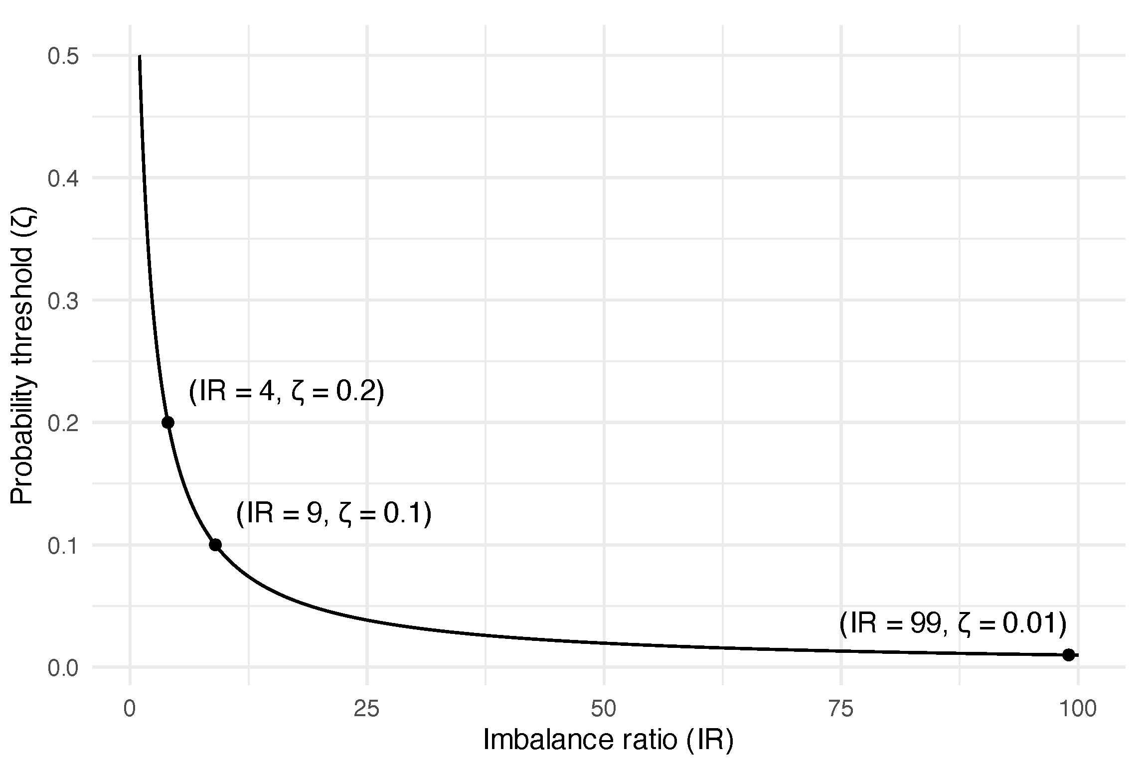
4.2. Probability Threshold Tuning

In the two-class case, MAP rule is equivalent to the use of a probability threshold ζ = 0.5 for assigning an observation to the minority class. Adjusting the threshold ζ ( 0 , 1 ) may serve as a simple solution in scenarios with different misclassification costs or in problems with imbalanced data. The classification rule entails assigning an observation x i to class C 1 if Pr ( C 1 | x i ) > ζ . However, the widely used default value ζ = 0.5 may not always yield the best results [17]. Optimal threshold selection can be accomplished, for instance, through cross-validation, hence choosing ζ CV as the value that maximizes a cross-validated suitable evaluation metric, such as F2 or balanced accuracy.
Another option is available by noting that, if the IR value is used for adjusting class-prior probabilities, as discussed in Section 4.1, the corresponding threshold value is simply obtained as
ζ IR = 1 1 + IR = τ ^ 1 ,
where τ ^ 1 is the sample proportion of cases in the minority class. Therefore, setting the threshold to match the proportion of the minority class in the training set is equivalent to a cost-sensitive approach using the cost matrix in Table 2b. Figure 1 depicts the relationship between IR and the corresponding probability threshold.
In accordance with this rationale, a threshold value can also be derived by employing the adjusted estimates of prior probabilities τ ˜ k , for  k = { 0 , 1 } , proposed by Saerens et al. [18]. This approach essentially employs an EM algorithm to iteratively update the posterior probabilities, enabling the computation of the adjusted prior probabilities and then setting ζ ADJ = τ ˜ 1 (for additional insights, refer to Scrucca et al. [12] (Section 4.6)).

4.3. Sampling Methods

Sampling techniques represent a data level approach for addressing class imbalance by sampling before applying classification models and algorithms [6]. Undersampling aims to reduce the number of instances from the majority class by randomly removing instances to restore balance. Conversely, oversampling involves replicating instances from the minority class to balance its representation with the majority class.
Beyond these approaches, other methods address class imbalance by generating synthetic samples for the minority class based on the existing data. For instance, SMOTE [19] generates synthetic samples by interpolating between existing instances of the minority class. The algorithm selects an observation from the minority class and finds its k-nearest neighbors in the feature space. Then, a synthetic instance is stochastically generated along the line segment in feature space that joins the original minority instance and a randomly chosen instance from among its neighbor. Let x i denote a minority class instance and x i represent one of its k-nearest neighbors. The synthetic case x new is generated as:
x new = x i + γ ( x i x i ) ,
where γ is a random value between 0 and 1. This process creates new instances along the line connecting x i and x i and is repeated until the desired balance between classes is achieved.
A related technique is ROSE [20], which generates artificial balanced samples according to a smoothed bootstrap approach. The ROSE algorithm estimates the underlying density distribution of the minority class by fitting a density function, such as a kernel density estimate, to the observed instances of the minority class. Once the density estimate is obtained, synthetic examples are generated by sampling from this estimated density centered at randomly chosen data points. Define the kernel density estimator as
f ^ H ( x ) = 1 n j = 1 n K H ( x x j ) ,
where H is the (symmetric and positive definite) smoothing matrix, K the kernel function (a symmetric multivariate density, often taken to be the standard multivariate Gaussian), and  K H ( x ) = | H | 1 / 2 K ( H 1 / 2 x ) . For a randomly chosen data points x i , ROSE generates a synthetic instance by sampling from the estimated density, i.e., 
x new f ^ H ( x i ) .
Thus, by employing density estimation to generate synthetic instances, ROSE aims to preserve the underlying distribution of the minority class while addressing class imbalance.
For a comprehensive overview of sampling methods for data imbalance see Fernández et al. [7] (Chapter 5).

5. Results

In this section, we delve into the impact of data imbalance on supervised GMMs. This exploration is carried out through simulation studies utilizing synthetic data [20], as well as two empirical analyses employing real-world data examples.

5.1. Simulation Studies

In the first simulated scenario, data have been generated by drawing from a mixture of bivariate Normal distributions with fixed means and covariance matrices. Following the notation in Murphy [21], the data generating process (DGP) can be described as follows:
y = { C 0 , C 1 } Cat ( τ ) x ( y = C k ) N ( μ k , Σ k ) .
According to the above DGP, classes are generated from the categorical distribution with probabilities τ = ( τ 0 , τ 1 ) , where Pr ( y = C k ) = τ k for k = { 0 , 1 } , and such that τ 0 + τ 1 = 1 . The majority class follows a bivariate standard Gaussian distribution, so μ 0 = 0 2 = 0 0 and Σ 0 = I 2 = 1 0 0 1 . Also, the minority class follows a bivariate Gaussian distribution, but with mean μ 1 = 1 1 and covariance matrix Σ 1 = 1 0.5 0.5 1 . In this simulation study, we consider samples of n = 5000 observations from the above DGP with the probability of the minority class τ 1 taken to be either 0.1 or 0.01 . After fitting models described in Section 2.2, their evaluation is based on a test set of size m = 50,000 generated from the same DGP. Results for 100 replications are reported in Table 3 and Table 4, while Figure 2 shows a sample of simulated data with decision boundaries for classification using different models and methods dealing with class imbalance.
Based on the results of this simulation study, it is clear that addressing class imbalance is important for both the EDDA model and the more flexible MclustDA model. The unbalanced distribution of classes significantly impacts the performance of these models, emphasizing the need for adjustment strategies. Furthermore, our findings indicate that the specific type of adjustment employed is only marginally relevant. Across various methods discussed in Section 4, a substantial enhancement in recall/sensitivity is observed, albeit at the expense of a slight decline in precision and specificity. This trade-off, while noteworthy, is offset by the substantial gains achieved in the correct identification of cases from the minority class.
In terms of thresholding strategies, our study demonstrates that cost-sensitive learning and optimal threshold value selected through cross-validation exhibit the most promising performance when evaluated using metrics such as the F2 score and balanced accuracy. This highlights the important role of thresholding in optimizing the models’ predictive power, particularly in scenarios with imbalanced class distributions. Among the sampling-based adjustments explored, the examined strategies demonstrate nearly comparable effectiveness. However, it is clear that downsampling stands out as the most straightforward and computationally efficient option in terms of implementation and computational speed.
The second simulated dataset is also generated from a mixture according to the following DGP:
y = { C 0 , C 1 } Cat ( τ ) x ( y = C 0 ) N ( 0 10 , I 10 ) x ( y = C 1 ) N ( 0 10 , I 10 ) x > 4 x 1 0 .
In this case, the majority class follows a 10-variate standard Gaussian distribution, while the rare class can be seen as a depleted semi-hypersphere filled with the prevalent class. Samples of n = 5000 observations are generated as training set from the above DGP with the probability of the minority class τ 1 taken to be either 0.1 or 0.01 . After fitting models described in Section 2.2, their evaluation is based on a test set of size m = 50,000 . Results from 100 replications are shown in Table 5 and Table 6.
In this simulation study, much like in the previous case, it is evident that addressing class imbalance is important for both the EDDA and MclustDA models. Class imbalance exerts a notable influence on model performance, reaffirming the need for the implementation of effective strategies to address this issue. In this simulated scenario, the relevance of the chosen adjustment becomes more apparent, particularly when dealing with a small prior probability for the minority class. Specifically, threshold adjustment emerges as the superior approach in comparison to sampling-based techniques to deal with class imbalance effectively, particularly in scenarios with severely imbalanced class distributions.
Looking deeply at the results, notable improvement in sensitivity is evident, a crucial aspect in correctly identifying the minority class, while simultaneously maintaining a substantial level of specificity. This striking balance ultimately leads to an enhanced measure of balanced accuracy, demonstrating the efficacy of the investigated adjustments. However, it is essential to note that both thresholding and sampling-based adjustments come at a cost: a significant decrease in precision coupled with an increase in recall. This trade-off, while substantial, necessitates a careful consideration of the specific priorities and objectives of the classification task.

5.2. Wine Quality Data

We consider the wine quality data [22] available from the UCI Machine Learning Data Repository [23]. The dataset contains data on 4898 white variants of the Portuguese “Vinho Verde” wine. For each wine, the results from 11 physicochemical tests are available, such as fixed, volatile, and citric acidity, residual sugar, chlorides, free and total sulfur dioxide, density, pH, sulphates, and alcohol. Moreover, the quality of each wine was assessed based on sensory data, with scores ranging from 0 to 10. For the present analysis, wines have been classified into two groups: those of High quality (with a score of at least 8) and those classified as MedLow quality (with a score less than 8). Notably, only 3.67 % of the wines achieved the distinction of high quality, leading to a clear imbalance between the classes.
The dataset was partitioned into a training set, which comprised approximately 2/3 of the wines, and a test set that encompassed the remaining 1/3 of total observations. Given that the proportion of the minority class is 0.0367 , the imbalance ratio in the training set is equal to IR = 26.22 .
Figure 3 illustrates the results derived from applying the models presented in Section 2.2, along with the remedies discussed in Section 4, to the test set. Without any adjustment for correcting class imbalance both the EDDA model and the MclustDA model have a quite low TPR, which leads to low values for recall and sensitivity. The precision and specificity are higher, but this does not compensate for the deficiency in detecting the minority class. Overall, both F2 and Balanced Accuracy are smaller for the unadjusted models that use the initial partition of the data.
Cost-sensitive predictions, as discussed in Section 4.1, employ the imbalance ratio mentioned above for both EDDA and MclustDA models. Recall that this is equivalent to use the proportion of the minority class as the classification threshold. Instead, optimal threshold for the EDDA model estimated by cross-validation is ζ CV = 0.08 , while using the adjusted prior probabilities, as discussed in Section 4.2, it is recalibrated as ζ ADJ = 0.299 . At the same time, for the MclustDA model the optimal threshold is estimated by cross-validation as ζ CV = 0.01 , while the adjusted threshold is estimated as ζ ADJ = 0.0501 . As shown in Figure 3, both the F2 score and balanced accuracy exhibit higher values when either the threshold-based approaches or the sampling-based approaches are employed to address class imbalance. While MclustDA models exhibit slightly better results compared to EDDA models, the variation among different methods for addressing imbalance is negligible. Therefore, the choice of the most effective approach to accommodate class imbalance should be guided by other considerations.

5.3. Hypothyroid Data

In this second data analysis example, we consider the hypothyroid dataset [24] available from the UCI Machine Learning Data Repository [23]. The dataset comprises information on 2012 patients, with 122 diagnosed as suffering from hypothyroidism. Age of patients and measures related to functioning of the thyroid gland, such as TSH, T3, TT4, T4U, and FTI, are used as features for classification.
Approximately 2/3 of the patients were randomly allocated to the training set, leaving the remaining 668 patients for the test set. The minority class proportion in the training set is equal to 0.0565 , resulting in an imbalance ratio of IR = 16.68 . In contrast, the test set exhibits a slightly higher proportion of the minority class at 0.0689 .
In Figure 4, the results obtained from fitting the models outlined in Section 2.2 and addressing data imbalance as discussed in Section 4 on the test set are presented. The EDDA model, devoid of any threshold-based or sample-based adjustments, exhibits the lowest sensitivity/recall (around 50%), resulting in both a less than satisfactory F2 score and balanced accuracy. In contrast, the MclustDA model, even without any correction for class imbalance, demonstrates noteworthy performance. Fine-tuning the threshold, particularly using ζ CV = 0.01 selected by cross-validation, or employing a sampling-based approach in the EDDA model, enhances the classification of the minority class. In the case of the MclustDA model, various adjustments result in marginal improvements, except for upsampling and SMOTE, which, conversely, lead to diminished performance compared to the unadjusted MclustDA model. This latter observation underlines that sampling-based approaches do not necessarily enhance classification accuracy.

6. Conclusions

Class imbalance can pose a significant challenge in many classification problems. In this paper, we investigated the effect of imbalanced data on supervised Gaussian mixture models (SGMMs) in classification problems. It has been established that this imbalance significantly hampers the performance of SGMMs, emphasizing the need for effective mitigation strategies.
This study specifically focuses on imbalanced two-class data, where the minority class is of primary importance, within the framework of Gaussian mixtures. The investigation centers on two prominent SGMMs, namely EDDA and MclustDA models. Additionally, a range of approaches to tackle class imbalance were presented, including threshold-based methods and sampling-based techniques.
The empirical results provide substantial insights into the necessity of addressing class imbalance for both the EDDA and MclustDA models. Notably, both threshold-based and sampling-based approaches exhibit marked improvements in classification accuracy for the minority class. Among these strategies, threshold-based adjustments, particularly those derived from cost-sensitive learning, stand out as highly recommended. This is due to their ability to enhance performance without necessitating model re-estimation, avoiding the loss of valuable training data, as in downsampling, or the artificial creation of data, as in oversampling techniques.
Table 7 offers a concise overview of various techniques explored in this paper for handling imbalanced data. Several crucial aspects deemed relevant in practical applications are considered, and a raw qualitative assessment is provided.
The contributions of this paper collectively serve as a valuable resource for practitioners and researchers, offering effective strategies to enhance the performance of supervised Gaussian mixtures in scenarios characterized by class imbalance.

Funding

This research received no external funding.

Data Availability Statement

All the analyses have been conducted in R [16] using the mclust package [14,15]. Code to reproduce the analyses is available in a GitHub repository at https://github.com/luca-scr/SGMM_Class_Imbalance (accessed on 15 October 2023).

Conflicts of Interest

The author declares no conflict of interest.

References

  1. McLachlan, G.J.; Peel, D. Finite Mixture Models; Wiley: New York, NY, USA, 2000. [Google Scholar]
  2. Fraley, C.; Raftery, A.E. Model-based Clustering, Discriminant Analysis, and Density Estimation. J. Am. Stat. Assoc. 2002, 97, 611–631. [Google Scholar] [CrossRef]
  3. McLachlan, G.J.; Lee, S.X.; Rathnayake, S.I. Finite Mixture Models. Annu. Rev. Stat. Appl. 2019, 6, 355–378. [Google Scholar] [CrossRef]
  4. Dempster, A.P.; Laird, N.M.; Rubin, D.B. Maximum likelihood from incomplete data via the EM algorithm (with discussion). J. R. Stat. Soc. Ser. B Stat. Methodol. 1977, 39, 1–38. [Google Scholar] [CrossRef]
  5. McLachlan, G.; Krishnan, T. The EM Algorithm and Extensions, 2nd ed.; Wiley-Interscience: Hoboken, NJ, USA, 2008. [Google Scholar]
  6. Sun, Y.; Wong, A.K.C.; Kamel, M.S. Classification of Imbalanced Data: A Review. Int. J. Pattern Recognit. Artif. Intell. 2009, 23, 687–719. [Google Scholar] [CrossRef]
  7. Fernández, A.; García, S.; Galar, M.; Prati, R.C.; Krawczyk, B.; Herrera, F. Learning from Imbalanced Data Sets; Springer: Berlin, Germany, 2018. [Google Scholar] [CrossRef]
  8. Pal, B.; Paul, M.K. A Gaussian mixture based boosted classification scheme for imbalanced and oversampled data. In Proceedings of the 2017 International Conference on Electrical, Computer and Communication Engineering (ECCE), Cox’s Bazar, Bangladesh, 6–18 February 2017; pp. 401–405. [Google Scholar] [CrossRef]
  9. Han, X.; Cui, R.; Lan, Y.; Kang, Y.; Deng, J.; Jia, N. A Gaussian mixture model based combined resampling algorithm for classification of imbalanced credit data sets. Int. J. Mach. Learn. Cybern. 2019, 10, 3687–3699. [Google Scholar] [CrossRef]
  10. Hastie, T.; Tibshirani, R. Discriminant analysis by Gaussian mixtures. J. R. Stat. Soc. Ser. B Stat. Methodol. 1996, 58, 155–176. [Google Scholar] [CrossRef]
  11. Bensmail, H.; Celeux, G. Regularized Gaussian Discriminant Analysis through Eigenvalue Decomposition. J. Am. Stat. Assoc. 1996, 91, 1743–1748. [Google Scholar] [CrossRef]
  12. Scrucca, L.; Fraley, C.; Murphy, T.B.; Raftery, A.E. Model-Based Clustering, Classification, and Density Estimation Using mclust in R; Chapman & Hall/CRC: New York, NY, USA, 2023. [Google Scholar] [CrossRef]
  13. Schwarz, G. Estimating the dimension of a model. Ann. Stat. 1978, 6, 461–464. [Google Scholar] [CrossRef]
  14. Scrucca, L.; Fop, M.; Murphy, T.B.; Raftery, A.E. mclust 5: Clustering, Classification and Density Estimation Using Gaussian Finite Mixture Models. R J. 2016, 8, 205–233. [Google Scholar] [CrossRef]
  15. Fraley, C.; Raftery, A.E.; Scrucca, L. mclust: Gaussian Mixture Modelling for Model-Based Clustering, Classification, and Density Estimation; R Package Version 6.0.0; R Foundation: Vienna, Austria, 2023. [Google Scholar]
  16. R Core Team. R: A Language and Environment for Statistical Computing; R Foundation: Vienna, Austria, 2022. [Google Scholar]
  17. Provost, F. Machine learning from imbalanced data sets 101. In Proceedings of the AAAI Workshop on Imbalanced Data Sets, Austin, TX, USA, 31 July 2000. [Google Scholar]
  18. Saerens, M.; Latinne, P.; Decaestecker, C. Adjusting the outputs of a classifier to new a priori probabilities: A simple procedure. Neural Comput. 2002, 14, 21–41. [Google Scholar] [CrossRef] [PubMed]
  19. Chawla, N.V.; Bowyer, K.W.; Hall, L.O.; Kegelmeyer, W.P. SMOTE: Synthetic minority over-sampling technique. J. Artif. Intell. Res. 2002, 16, 321–357. [Google Scholar] [CrossRef]
  20. Menardi, G.; Torelli, N. Training and assessing classification rules with imbalanced data. Data Min. Knowl. Discov. 2012, 28, 92–122. [Google Scholar] [CrossRef]
  21. Murphy, K.P. Probabilistic Machine Learning: An Introduction; MIT Press: Cambridge, MA, USA, 2022. [Google Scholar]
  22. Cortez, P.; Cerdeira, A.; Almeida, F.; Matos, T.; Reis, J. Wine Quality Data; UCI Machine Learning Repository; UC Irvine: Irvine, CA, USA, 2009. [Google Scholar] [CrossRef]
  23. Dua, D.; Graff, C. UCI Machine Learning Repository. 2019. Available online: http://archive.ics.uci.edu/ml (accessed on 14 September 2023).
  24. Quinlan, R. Thyroid Disease; UCI Machine Learning Repository; UC Irvine: Irvine, CA, USA, 1987. [Google Scholar] [CrossRef]
Figure 1. Relationship between probability threshold and imbalance ratio.
Algorithms 16 00563 g001
Figure 2. Decision boundaries for classification of data generated according to the first simulated scenario corresponding to different models and methods addressing class imbalance.
Algorithms 16 00563 g002
Figure 3. Performance outcomes for various models and methods addressing class imbalance on the wine quality dataset.
Algorithms 16 00563 g003
Figure 4. Performance outcomes for various models and methods addressing class imbalance on the hypothyroid dataset.
Algorithms 16 00563 g004
Table 1. Confusion matrix for two-class data.
Actual/Observed
NegativePositive
Predicted       
NegativeTrue Negative (TN)False Negative (FN)
PositiveFalse Positive (FP)True Positive (TP)
Table 2. Cost matrix for binary-class data.
(a) Generic case
Actual/Observed
NegativePositive
Predicted
Negative c ( 0 | 0 ) c ( 0 | 1 )
Positive c ( 1 | 0 ) c ( 1 | 1 )
(b) Imbalance ratio (IR) case
Actual/Observed
NegativePositive
Predicted
Negative01
PositiveIR0
Table 3. Results for the first simulated scenario with probability of the minority class τ 1 = 0.01 for various models and methods addressing class imbalance. Values reported are averages (with standard errors in parentheses) obtained from simulations.
MethodPrecision/
PPV
Recall/
TPR
F2Sensitivity/
TPR
Specificity/
TNR
Balanced Accuracy
EDDA0.0289 (0.0094)0.0002 (0.0001)0.0003 (0.0001)0.0002 (0.0001)0.9999 (0.0000)0.5001 (0.0000)
EDDA+costSens0.0339 (0.0002)0.8347 (0.0025)0.1457 (0.0009)0.8347 (0.0025)0.7612 (0.0017)0.7979 (0.0010)
EDDA+adjPriorThreshold0.0254 (0.0011)0.9030 (0.0097)0.1113 (0.0041)0.9030 (0.0097)0.5488 (0.0273)0.7259 (0.0103)
EDDDA+optThreshold0.0350 (0.0005)0.8221 (0.0056)0.1489 (0.0015)0.8221 (0.0056)0.7685 (0.0040)0.7953 (0.0013)
EDDA+downSamp0.0330 (0.0004)0.8391 (0.0037)0.1421 (0.0014)0.8391 (0.0037)0.7503 (0.0034)0.7947 (0.0015)
EDDA+upSamp0.0335 (0.0003)0.8491 (0.0027)0.1446 (0.0011)0.8491 (0.0027)0.7535 (0.0023)0.8013 (0.0010)
EDDA+smote0.0335 (0.0003)0.8408 (0.0032)0.1442 (0.0012)0.8408 (0.0032)0.7551 (0.0027)0.7980 (0.0012)
MCLUSTDA0.1190 (0.0251)0.0009 (0.0002)0.0011 (0.0002)0.0009 (0.0002)1.0000 (0.0000)0.5004 (0.0001)
MCLUSTDA+costSens0.0335 (0.0003)0.8416 (0.0032)0.1443 (0.0011)0.8416 (0.0032)0.7553 (0.0025)0.7985 (0.0012)
MCLUSTDA+adjPriorThreshold0.0295 (0.0010)0.8685 (0.0094)0.1272 (0.0039)0.8685 (0.0094)0.6388 (0.0239)0.7537 (0.0087)
MCLUSTDA+optThreshold0.0359 (0.0006)0.8144 (0.0068)0.1514 (0.0017)0.8144 (0.0068)0.7745 (0.0045)0.7944 (0.0017)
MCLUSTDA+downSamp0.0326 (0.0004)0.8472 (0.0039)0.1409 (0.0014)0.8472 (0.0039)0.7446 (0.0037)0.7959 (0.0016)
MCLUSTDA+upSamp0.0332 (0.0005)0.7019 (0.0072)0.1390 (0.0018)0.7019 (0.0072)0.7919 (0.0032)0.7469 (0.0033)
MCLUSTDA+smote0.0333 (0.0005)0.6867 (0.0071)0.1390 (0.0019)0.6867 (0.0071)0.7970 (0.0032)0.7419 (0.0032)
Table 4. Results for the first simulated scenario with probability of the minority class τ 1 = 0.1 for various models and methods addressing class imbalance. Values reported are averages (with standard errors in parentheses) obtained from simulations.
MethodPrecision/
PPV
Recall/
TPR
F2Sensitivity/
TPR
Specificity/
TNR
Balanced
Accuracy
EDDA0.5539 (0.0024)0.1478 (0.0030)0.1726 (0.0033)0.1478 (0.0030)0.9866 (0.0003)0.5672 (0.0013)
EDDA+costSens0.2782 (0.0006)0.8508 (0.0009)0.6026 (0.0005)0.8508 (0.0009)0.7551 (0.0008)0.8029 (0.0003)
EDDA+adjPriorThreshold0.2748 (0.0009)0.8566 (0.0014)0.6015 (0.0005)0.8566 (0.0014)0.7488 (0.0014)0.8027 (0.0003)
EDDDA+optThreshold0.2781 (0.0018)0.8498 (0.0030)0.6008 (0.0007)0.8498 (0.0030)0.7534 (0.0029)0.8016 (0.0003)
EDDA+downSamp0.2773 (0.0006)0.8523 (0.0010)0.6023 (0.0005)0.8523 (0.0010)0.7535 (0.0009)0.8029 (0.0003)
EDDA+upSamp0.2768 (0.0006)0.8542 (0.0009)0.6027 (0.0005)0.8542 (0.0009)0.7524 (0.0008)0.8033 (0.0003)
EDDA+smote0.2763 (0.0006)0.8547 (0.0009)0.6024 (0.0005)0.8547 (0.0009)0.7516 (0.0008)0.8032 (0.0003)
MCLUSTDA0.5753 (0.0030)0.1211 (0.0037)0.1430 (0.0041)0.1211 (0.0037)0.9897 (0.0004)0.5554 (0.0017)
MCLUSTDA+costSens0.2764 (0.0006)0.8551 (0.0009)0.6026 (0.0005)0.8551 (0.0009)0.7515 (0.0008)0.8033 (0.0003)
MCLUSTDA+adjPriorThreshold0.2740 (0.0008)0.8588 (0.0013)0.6017 (0.0005)0.8588 (0.0013)0.7473 (0.0013)0.8031 (0.0003)
MCLUSTDA+optThreshold0.2782 (0.0017)0.8506 (0.0029)0.6013 (0.0006)0.8506 (0.0029)0.7534 (0.0028)0.8020 (0.0003)
MCLUSTDA+downSamp0.2762 (0.0006)0.8550 (0.0010)0.6023 (0.0005)0.8550 (0.0010)0.7513 (0.0009)0.8031 (0.0003)
MCLUSTDA+upSamp0.2763 (0.0010)0.8497 (0.0016)0.6001 (0.0006)0.8497 (0.0016)0.7526 (0.0016)0.8011 (0.0004)
MCLUSTDA+smote0.2752 (0.0010)0.8490 (0.0017)0.5987 (0.0006)0.8490 (0.0017)0.7514 (0.0016)0.8002 (0.0004)
Table 5. Results for the second simulated scenario with probability of the minority class τ 1 = 0.01 for various models and methods addressing class imbalance. Values reported are averages (with standard errors in parentheses) obtained from simulations.
MethodPrecision/
PPV
Recall/
TPR
F2Sensitivity/
TPR
Specificity/
TNR
Balanced
Accuracy
EDDA0.8096 (0.0040)0.3336 (0.0042)0.3774 (0.0044)0.3336 (0.0042)0.9992 (0.0000)0.6664 (0.0021)
EDDA+costSens0.0912 (0.0014)0.9103 (0.0054)0.3242 (0.0040)0.9103 (0.0054)0.9050 (0.0022)0.9077 (0.0033)
EDDA+adjPriorThreshold0.0856 (0.0013)0.9192 (0.0072)0.3105 (0.0035)0.9192 (0.0072)0.8988 (0.0015)0.9090 (0.0034)
EDDDA+optThreshold0.0968 (0.0021)0.8988 (0.0071)0.3340 (0.0048)0.8988 (0.0071)0.9101 (0.0025)0.9045 (0.0035)
EDDA+downSamp0.0617 (0.0020)0.8914 (0.0122)0.2386 (0.0066)0.8914 (0.0122)0.8488 (0.0046)0.8701 (0.0075)
EDDA+upSamp0.0835 (0.0008)0.8007 (0.0045)0.2940 (0.0020)0.8007 (0.0045)0.9102 (0.0010)0.8555 (0.0021)
EDDA+smote0.0653 (0.0013)0.6305 (0.0094)0.2297 (0.0040)0.6305 (0.0094)0.9062 (0.0017)0.7684 (0.0048)
MCLUSTDA0.8470 (0.0038)0.3046 (0.0027)0.3491 (0.0028)0.3046 (0.0027)0.9994 (0.0000)0.6520 (0.0013)
MCLUSTDA+costSens0.0861 (0.0006)0.9055 (0.0023)0.3116 (0.0015)0.9055 (0.0023)0.9022 (0.0008)0.9038 (0.0010)
MCLUSTDA+adjPriorThreshold0.0717 (0.0012)0.9374 (0.0035)0.2725 (0.0034)0.9374 (0.0035)0.8727 (0.0026)0.9051 (0.0010)
MCLUSTDA+optThreshold0.0925 (0.0021)0.8923 (0.0053)0.3220 (0.0039)0.8923 (0.0053)0.9067 (0.0021)0.8995 (0.0017)
MCLUSTDA+downSamp0.0557 (0.0011)0.9292 (0.0047)0.2231 (0.0033)0.9292 (0.0047)0.8343 (0.0034)0.8817 (0.0022)
MCLUSTDA+upSamp0.0451 (0.0017)0.1121 (0.0081)0.0815 (0.0049)0.1121 (0.0081)0.9783 (0.0012)0.5452 (0.0036)
MCLUSTDA+smote0.0471 (0.0017)0.0845 (0.0047)0.0703 (0.0033)0.0845 (0.0047)0.9828 (0.0007)0.5337 (0.0021)
Table 6. Results for the second simulated scenario with probability of the minority class τ 1 = 0.1 for various models and methods addressing class imbalance. Values reported are averages (with standard errors in parentheses) obtained from simulations.
MethodPrecision/
PPV
Recall/
TPR
F2Sensitivity/
TPR
Specificity/
TNR
Balanced
Accuracy
EDDA0.8554 (0.0009)0.6067 (0.0013)0.6441 (0.0011)0.6067 (0.0013)0.9886 (0.0001)0.7976 (0.0006)
EDDA+costSens0.5292 (0.0009)0.9469 (0.0009)0.8177 (0.0005)0.9469 (0.0009)0.9064 (0.0003)0.9266 (0.0004)
EDDA+adjPriorThreshold0.5230 (0.0012)0.9511 (0.0008)0.8172 (0.0005)0.9511 (0.0008)0.9036 (0.0004)0.9274 (0.0003)
EDDDA+optThreshold0.4904 (0.0024)0.9701 (0.0013)0.8107 (0.0008)0.9701 (0.0013)0.8874 (0.0012)0.9288 (0.0003)
EDDA+downSamp0.5255 (0.0013)0.9609 (0.0012)0.8241 (0.0006)0.9609 (0.0012)0.9035 (0.0006)0.9322 (0.0005)
EDDA+upSamp0.5221 (0.0009)0.9498 (0.0009)0.8160 (0.0005)0.9498 (0.0009)0.9034 (0.0004)0.9266 (0.0003)
EDDA+smote0.5039 (0.0009)0.9231 (0.0015)0.7913 (0.0009)0.9231 (0.0015)0.8990 (0.0004)0.9110 (0.0006)
MCLUSTDA0.8550 (0.0009)0.6119 (0.0022)0.6487 (0.0019)0.6119 (0.0022)0.9885 (0.0001)0.8002 (0.0011)
MCLUSTDA+costSens0.5110 (0.0016)0.9596 (0.0014)0.8159 (0.0005)0.9596 (0.0014)0.8978 (0.0008)0.9287 (0.0004)
MCLUSTDA+adjPriorThreshold0.5134 (0.0015)0.9589 (0.0012)0.8168 (0.0006)0.9589 (0.0012)0.8989 (0.0006)0.9289 (0.0004)
MCLUSTDA+optThreshold0.4979 (0.0036)0.9679 (0.0017)0.8129 (0.0013)0.9679 (0.0017)0.8903 (0.0017)0.9291 (0.0004)
MCLUSTDA+downSamp0.5043 (0.0016)0.9576 (0.0016)0.8113 (0.0007)0.9576 (0.0016)0.8952 (0.0008)0.9264 (0.0005)
MCLUSTDA+upSamp0.5136 (0.0015)0.8717 (0.0028)0.7648 (0.0019)0.8717 (0.0028)0.9082 (0.0005)0.8900 (0.0013)
MCLUSTDA+smote0.4946 (0.0013)0.8108 (0.0027)0.7187 (0.0019)0.8108 (0.0027)0.9079 (0.0005)0.8593 (0.0013)
Table 7. Summary of specific techniques for handling imbalanced two-class data in supervised GMMs (higher number of indicates better rating; — indicates not applicable).
TechniquesAccuracyComputational
Speed
Ease of ImplementationHyperparameter TuningScalabilityParallelization
costSens
adjPriorThreshold
optThreshold
downSamp
upSamp
smote
Disclaimer/Publisher’s Note: The statements, opinions and data contained in all publications are solely those of the individual author(s) and contributor(s) and not of MDPI and/or the editor(s). MDPI and/or the editor(s) disclaim responsibility for any injury to people or property resulting from any ideas, methods, instructions or products referred to in the content.

