Period Cycle Optimization of Integrated Energy Systems with Long-Term Scheduling Consideration

Abstract

The economy and energy saving effects of integrated energy system dispatch plans are influenced by the coupling of different energy devices. In order to consider the impact of changes in equipment load rates on the optimization and scheduling of the system under long-term operation, a method for energy and component cycle optimization considering energy device capacity and load has been proposed. By improving the initial parameters of the components, energy economic parameters, and operational optimization parameters, the system is subjected to long-term scheduling and multi-cycle operational optimization analysis to evaluate the energy saving and emission reduction potential as well as the economic feasibility of the system. Finally, through numerical analysis, the effectiveness of this optimization approach in achieving energy savings, emission reductions, and cost benefits for the system is validated. Furthermore, compared to existing optimization methods, this approach also assesses the economic feasibility of the system. The case study resulted in a pre-tax IRR of 23.14% and a pre-tax NPV of 66.38 million. It is inferred that the system could generate profits over a 10-year operation period, thereby offering a more rational and cost-effective scheduling scheme for the integrated energy system.

1. Introduction

The current global energy consumption pattern is gradually becoming diversified and automated [1]. A single energy source is no longer able to meet users’ demands [2]. Traditional energy sources have also formed their own systems and independently carried out production and supply [3], leading to a series of issues such as high energy consumption and low efficiency, as well as security concerns. With the changing global energy landscape and scientific and technological innovation [4], there is an increasing proposal to establish an interconnected energy system that integrates traditional and new energy sources to achieve integrated production, transportation, consumption, and storage of various types of energy [5].

The latest energy system designs are increasingly aimed at integrating renewable or low-carbon energy sources to reduce costs and decrease greenhouse gas emissions [6]. Nie et al. [7] designed a home power energy management system using solar renewable energy, which effectively reduces the cost of energy usage in smart homes. Wang et al. [8] utilized energy efficiency measures (EEMs) and photovoltaic (PV) cells to reduce energy consumption and carbon emissions for all types of buildings, alleviating the community’s peak electricity load. Wang et al. [9] proposed a hydrogen-based integrated energy system as the primary clean energy source, significantly reducing operational costs and carbon emissions. Naili et al. [10] utilized solar-assisted ground source heat pump systems to enhance the performance of energy systems. Over the past decade, energy systems have evolved from initially being based on electricity and heat to focusing on thermal balance, integrating various types of energy sources and employing techniques such as energy storage and intelligent control to achieve the integrated intelligent control of energy [11]. Favre-Perrod introduced the concept of energy hubs [12] early on, which are multi-energy systems that connect different types of energy producers and consumers, leveraging energy conversion technology and storage to facilitate energy supply planning. Geidl [13] further investigated this concept by establishing modeling and optimization methods and studying the interconnection of multiple energy sources in a network.

Renewable energy sources, in comparison to fossil fuels, are less amenable to storage and exhibit an uneven temporal distribution with a high degree of randomness. Within integrated energy systems, various energy flows are interconnected, presenting considerable uncertainty in their utilization. As the proportion and diversity of renewable energy sources continue to grow, energy system operation scenarios encounter uncertainty stemming from both consumer behavior and energy source variability [14,15]. Consequently, to enhance the design of integrated energy systems, it becomes imperative to develop an optimization methodology capable of accommodating the diversity of operational scenarios and optimizing operational continuity [16].

In addition to considering the instability of renewable energy and the interactions between different energy sources, various issues need to be taken into account, such as the environment and the power of energy equipment. This will also result in a highly complex system. Therefore, various optimization methods can be employed in the design of integrated energy systems to enhance system complexity, reduce modeling efforts, and improve reusability [6,17,18]. Tonellato et al. [19] developed an integrated optimization approach based on MILP (Mixed-Integer Linear Programming) to optimize various energy systems, aiming to minimize overall costs and enhance efficiency. Miglani et al. [20] utilized a dual-layer integrated optimization method based on a GA (genetic algorithm) and MILP to optimize a comprehensive energy system consisting of ground source heat pumps and solar collectors, with the objective of reducing the total costs and carbon emissions. Jin et al. [21] developed a multi-objective system optimization model to design strategies for electrical load (FEL) and thermal load (FTL), aiming to enhance system efficiency and reduce overall costs. Song et al. [22] employed a multi-objective bi-level optimization approach to improve the feasibility and overall benefits of planning schemes. Nie et al. [7] utilized an Improved Particle Swarm Optimization method (ILPSO) to reduce the peak-to-average ratio (PAR) and energy usage costs in smart homes. Liu et al. [23] employed a multi-objective operational optimization algorithm to decrease the operational costs of agricultural integrated energy systems while enhancing the photovoltaic penetration rate. Zhang et al. [24] proposed an electric–thermal coupling interconnect structure and an energy flow model for establishing a multi-energy complementary system in oilfield well sites. Additionally, a dynamic optimization method for source-load storage was employed to achieve overall performance scheduling of the system.

The aforementioned achievements have laid a solid foundation for the research presented in this paper. However, considering the need for further in-depth exploration in the existing literature regarding energy equipment capacity, load variations, and long-term system scheduling optimization, as well as the limited discussion on the economic evaluation of systems, this paper aims to investigate performance optimization and economic feasibility issues in the long-term scheduling of integrated energy systems. A methodology based on genetic algorithms and deep learning is proposed for energy and component cycle optimization, which divides the system’s long-term operating time into multiple operating periods and dynamically captures the component load conditions, energy dynamic interference, and response during each period. Through long-term, multi-period optimization in computational examples, real-time scheduling data, energy saving and emission reduction effects, and economic feasibility are obtained, thereby verifying the improved operational benefits of long-term scheduling optimization for the system.

2. Materials and Methods

2.1. System’s Optimization Algorithms

2.1.1. Objective Function

Minimizing the total energy consumption ($Q_{total}$), total energy cost ($C_{total}$), and total carbon emissions ($E_{total}$) represents the ultimate goal of this system. The load rate ($lr$) of each component serves as a critical decision variable for these parameters, allowing for the optimization of energy structure, component capacities, and load rates to achieve the best possible outcomes.

$$\begin{array}{c}min{Q}_{total}=f_1\left(l{r}_1,l{r}_2,\cdots ,l{r}_n\right)\\ min{C}_{total}=f_2\left(l{r}_1,l{r}_2,\cdots ,l{r}_n\right)\\ min{E}_{total}=f_3\left(l{r}_1,l{r}_2,\cdots ,l{r}_n\right)\\ 0\ll l{r}_i\ll l{r}_{i,max },i=1,2,\cdots ,m\\ g_k\left(l{r}_1,l{r}_2,\cdots ,l{r}_n\right)\ll 0,k=1,2,\cdots ,m\end{array}$$

(1)

where $f$ is the objective function, $i$ is different energy components, $g$ is the constraint function, $n$ is the number of decision variables, and $m$ is the number of constraint functions.

The overall gain of the system, which serves as the economic objective, aims to enhance the system’s competitiveness by maximizing its economic efficiency while fulfilling the ultimate goal. The optimization of the objective function leads to the maximization of the overall gain of the system.

$$G=max\left[\left(INCOM{E}_{bene}+INCOM{E}_{resi}\right)-\left(COS{T}_{inve}+COS{T}_{oper}+COS{T}_{depr}+COS{T}_{fuel}\right)\right]$$

(2)

$$INCOM{E}_{bene}={\displaystyle \sum }_{b\in B}{\displaystyle \sum }_{t\in T}{k}_{b,t}^{sell}\times P_{b,t}^{sell}\times \mathsf{\Delta }{t}_t$$

(3)

$$INCOM{E}_{resi}={\displaystyle \sum }_{c\in C^{prod,stor}}{\displaystyle \sum }_{t\in T}{k}_{c,t}^{resi}\times {\epsilon }_{c,t}$$

(4)

$$COS{T}_{inve}={\displaystyle \sum }_{c\in C^{prod}}\frac{k_c^{inv,prod}}{pv{f}_c}\times P_c^{prod}+{\displaystyle \sum }_{c\in C^{stor}}\frac{k_c^{inv,stor}}{pv{f}_c}\times P_c^{stor}$$

(5)

$$COS{T}_{oper}={\displaystyle \sum }_{s\in S}{\displaystyle \sum }_{t\in T}{\displaystyle \sum }_{c\in C^{prod}}{k}_c^{prod}\times P_{s,t,c}^{prod,load}\times \mathsf{\Delta }{t}_t+{\displaystyle \sum }_{b\in B}{\displaystyle \sum }_{t\in T}{\displaystyle \sum }_{c\in C^{stor}}{k}_c^{stor}\times P_{b,t,c}^{stor,load}\times \mathsf{\Delta }{t}_t$$

(6)

$$COS{T}_{depr}={\displaystyle \sum }_{c\in C^{prod,stor}}{\displaystyle \sum }_{t\in T}{k}_{c,t}^{depr}\times {\phi }_{c,t}$$

(7)

$$COS{T}_{fuel}={\displaystyle \sum }_{b\in B}{\displaystyle \sum }_{t\in T}{k}_{b,t}^{buy}\times P_{b,t}^{buy}\times \mathsf{\Delta }{t}_t$$

(8)

where $G$ is the system’s overall gain, $INCOME$ is the system’s total income, $COST$ is the system’s total expenses, $C$ is the total equipment, $pvf$ is the present value factor for specific components of the equipment, $P$ is the flow of energy, $k$ is cost, $\phi$ is the depreciation coefficient of the equipment, and $\epsilon$ is the equipment residual value coefficient. The superscript $prod$ is production, $stor$ is energy storage, $buy$ is energy purchase, $depr$ is fixed asset depreciation, $resi$ is equipment residual value, and $sell$ is energy sales. The subscript $c$ is each individual piece of equipment, $b\in B$ is the system’s energy demand, $s\in S$ is load intervals, and $t\in T$ is time steps.

2.1.2. Constraint Conditions

In this system, the load ratios of various components are constrained by the balance of different resources, power generation, energy storage, and supply.

For solar photovoltaic panels, their electrical output is nonlinearly correlated with solar radiation, which can be described by the following calculation formula:

$$p{v}_{elec}=p{v}_{capa}\times lr=p{v}_{capa}\times f\left(si\right)$$

(9)

where $pv$, $hm$, $br$, $cu$, $gb$, $pg$, $ng$, $wt$, and $hp$ are the photovoltaics, refrigeration unit, lithium bromide absorption chiller, CHP, gas boiler, power grid, natural gas station, wind turbine, and ground source heat pump, $elec$, $heat$, $cold$, and $gas$ represent electricity, heat, cool, and gas loads, $capa$ is the capacity of the energy component, $si$ is solar radiation in kW, and $sp$ is wind speed in m/s.

For the wind turbine, its electrical output is nonlinearly related to wind speed.

$$w{t}_{elec}=w{t}_{capa}\times lr=w{t}_{capa}\times f\left(sp\right)$$

(10)

For the ground source heat pump, its electrical input is nonlinearly related to its load rate.

$$h{p}_{elec}=\left(h{p}_{capa}\times lr\right)/f\left(lr\right)$$

(11)

For airborne main engines and double-working condition main engines, their electrical input is nonlinearly related to their load rate.

$$h{m}_{elec}=\left(h{m}_{capa}\times lr\right)/f\left(lr\right)$$

(12)

For lithium bromide refrigeration machines, their heat input is nonlinearly related to their load rate.

$$b{r}_{heat}=\left(b{r}_{capa}\times lr\right)/f\left(lr\right)$$

(13)

For CHP and gas boilers, their gas flow rate is nonlinearly related to their load rate.

$$c{u}_{gas}=\left(c{u}_{capa}\times lr\right)/f\left(lr\right)$$

(14)

$$g{b}_{gas}=\left(g{b}_{capa}\times lr\right)/f\left(lr\right)$$

(15)

The power grid can be regarded as a flexible generator with constant efficiency, and its output can be calculated with Equation (22), with the output power not exceeding its maximum carrying capacity.

$$p{g}_{out}\le max\left(p{g}_{capa},p{g}_{out}\right)$$

(16)

where $p{g}_{out}$ is the electrical output power from the grid in kWh.

The CHP and gas boilers are dispatchable variables; the output power of the natural gas station is calculated with Equation (25).

$$n{g}_{out}\le max\left(n{g}_{capa},n{g}_{out}\right)$$

(17)

where $p{g}_{out}$ represents the natural gas flow rate, and the gas flow rate (m³/h) is converted into power (kW) by using the calorific value of natural gas (kWh/m³).

The energy storage and output power within a certain period can be expressed as shown in Equation (18), with the maximum energy storage and power transmission conditions subjected to the constraints of Equations (20) and (21).

$$s{t}_i=\frac{s{t}_i^c}{{\eta }^c}{\delta }_c\left(s{t}_i^{total}\right)-s{t}_i^d{\eta }^d{\delta }_d\left(s{t}_i^{total}\right)$$

(18)

$$0\ll s{t}_i^{total}\ll s{t}_{i,max}^{total}$$

(19)

$$0\ll \frac{s{t}_i^c\left(t\right)}{{\eta }^c}\ll s{t}_{i,max}^c\left(t\right){\delta }_c\left(s{t}_i^{total}\right)$$

(20)

$$0\ll s{t}_i^d\left(t\right){\eta }^d\ll s{t}_{i,max}^d\left(t\right){\eta }^d{\delta }_d\left(s{t}_i^{total}\right)$$

(21)

where $s{t}_i^{total}$ is the total stored energy of each piece of energy storage equipment, $s{t}_i$ is the energy storage power within a certain time period, ${\eta }^c$ is the energy storage efficiency of the energy storage component, ${\eta }^d$ is the energy transfer efficiency of the energy storage component, $t$ is the duration of energy storage and transfer for the energy storage component, $i$ is the number of components, and ${\delta }_c$ and ${\delta }_d$ denote the efficient storage and output energy related to the total energy storage, respectively.

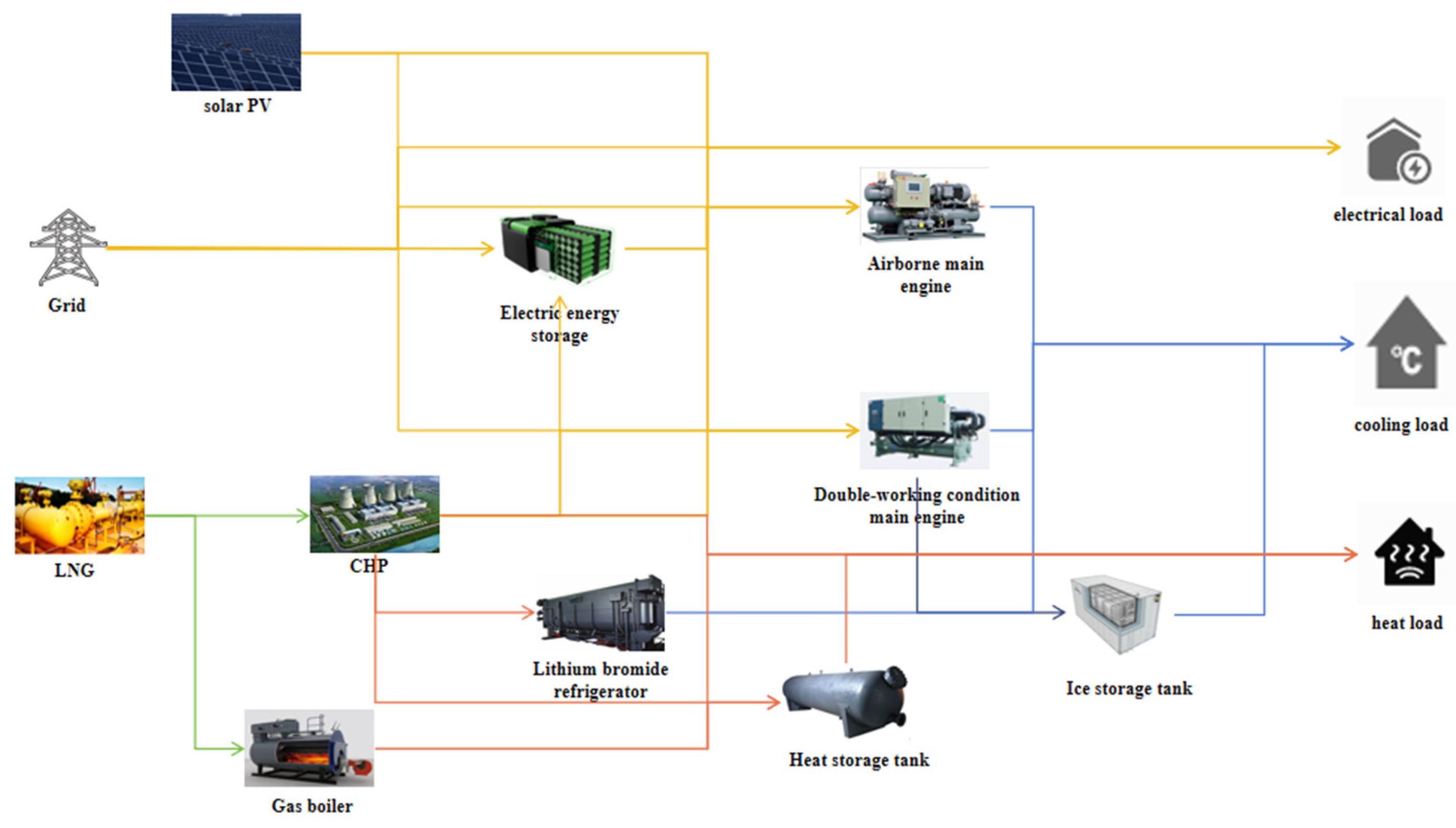
In the integrated energy systems, electricity is the most commonly used energy source, and its energy structure is also the most complex. The electricity balance equation for it is as follows:

$$p{g}_{elec}+p{v}_{elec}+c{u}_{elec}+s{t}_{elec,out}=l{d}_{elec}+h{m}_{elec}+s{t}_{elec,in}$$

(22)

where $ld$ is the power consumed by the user, which refers to the power inputted into the user load. Its unit is kW.

Its heat energy balance equation is as follows:

$$g{b}_{heat,out}+c{u}_{heat}+s{t}_{heat,out}=l{d}_{heat}+b{r}_{heat,in}+s{t}_{heat,in}$$

(23)

The cold energy balance equation is as follows:

$$b{r}_{cold}+h{m}_{cold}+s{t}_{cold,out}=l{d}_{cold}+s{t}_{cold,in}$$

(24)

Due to the widespread adoption and utilization of natural gas, many energy systems now incorporate natural gas as a primary clean energy source. This system will also introduce gas equilibrium considerations:

$$n{g}_{gas}=g{b}_{gas}+c{u}_{gas}$$

(25)

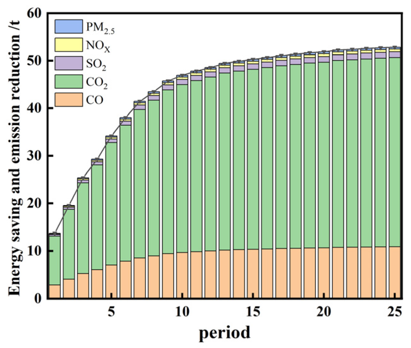
The external energy consumption of the system comprises electricity and natural gas. By considering the consumption factors, energy prices, and emission factors associated with these two energy sources, the energy consumption ($Q_{re}$), energy costs ($C_{re}$), and carbon emissions ($E_{re}$) can be calculated.

$$\begin{array}{c}{Q}_{re}=t\times p{g}_{out}\times q_{pg}+t\times n{g}_{out}\\ C_{re}=t\times p{g}_{out}\times P_{pg}+t\times n{g}_{out}\times P_{pg}\\ E_{re}=t\times p{g}_{out}\times e_{pg}+t\times n{g}_{out}\times e_{pg}\end{array}$$

(26)

where $Q$ is energy consumption in kWh, $C$ is the energy cost in dollars, $E$ is carbon emissions in kg, $t$ is the duration of continuous operation in hours, $q$ is the consumption factor, $P$ is energy prices in dollars/kWh, and $e$ is the emission factor in kg/kWh.

The system utilizes energy storage in the form of stored energy, which incurs corresponding energy consumption ($Q_{st}$) during the storage process. This consumption is mainly associated with the power and consumption factors of all storage components. The energy released from the storage components is considered a positive value of power, which implies an increase in energy consumption, carbon emissions, and energy cost. Similarly, the energy input into the storage components is represented by negative power, which reduces energy consumption, carbon emissions, and energy costs. Therefore, $Q_{st}$ can be positive or negative. Additionally, the cost ($C_{st}$) and carbon emissions ($E_{st}$) of storing energy can be calculated.

$$\begin{array}{c}{Q}_{st}={\displaystyle {\displaystyle \sum }_i}t\times P_{st}\times q_{st,i}\\ C_{st}={\displaystyle {\displaystyle \sum }_i}t\times P_{st}\times p_{st,i}\\ E_{st}={\displaystyle {\displaystyle \sum }_i}t\times P_{st}\times e_{st,i}\end{array}$$

(27)

where $P_{st}$ is the charge and discharge power in kW.

Additionally, the system incorporates surplus energy selling as a means to capitalize on price differentials, particularly in peak and off-peak electricity pricing, by choosing to sell excess energy during off-peak hours, thereby reducing energy costs. Consequently, the total energy consumption ($Q_{total}$) at a given time encompasses the consumption of energy resources ($Q_{re}$), storage energy ($Q_{st}$), and the revenue generated from selling energy ($Q_{sell}$). Similarly, total energy costs ($C_{total}$) and carbon emissions ($E_{total}$) can be computed.

$$\begin{array}{c}{Q}_{total}=Q_{re}+Q_{st}-Q_{sell}\\ C_{total}=C_{re}+C_{st}-C_{sell}\\ E_{total}=E_{re}+E_{st}-E_{sell}\end{array}$$

(28)

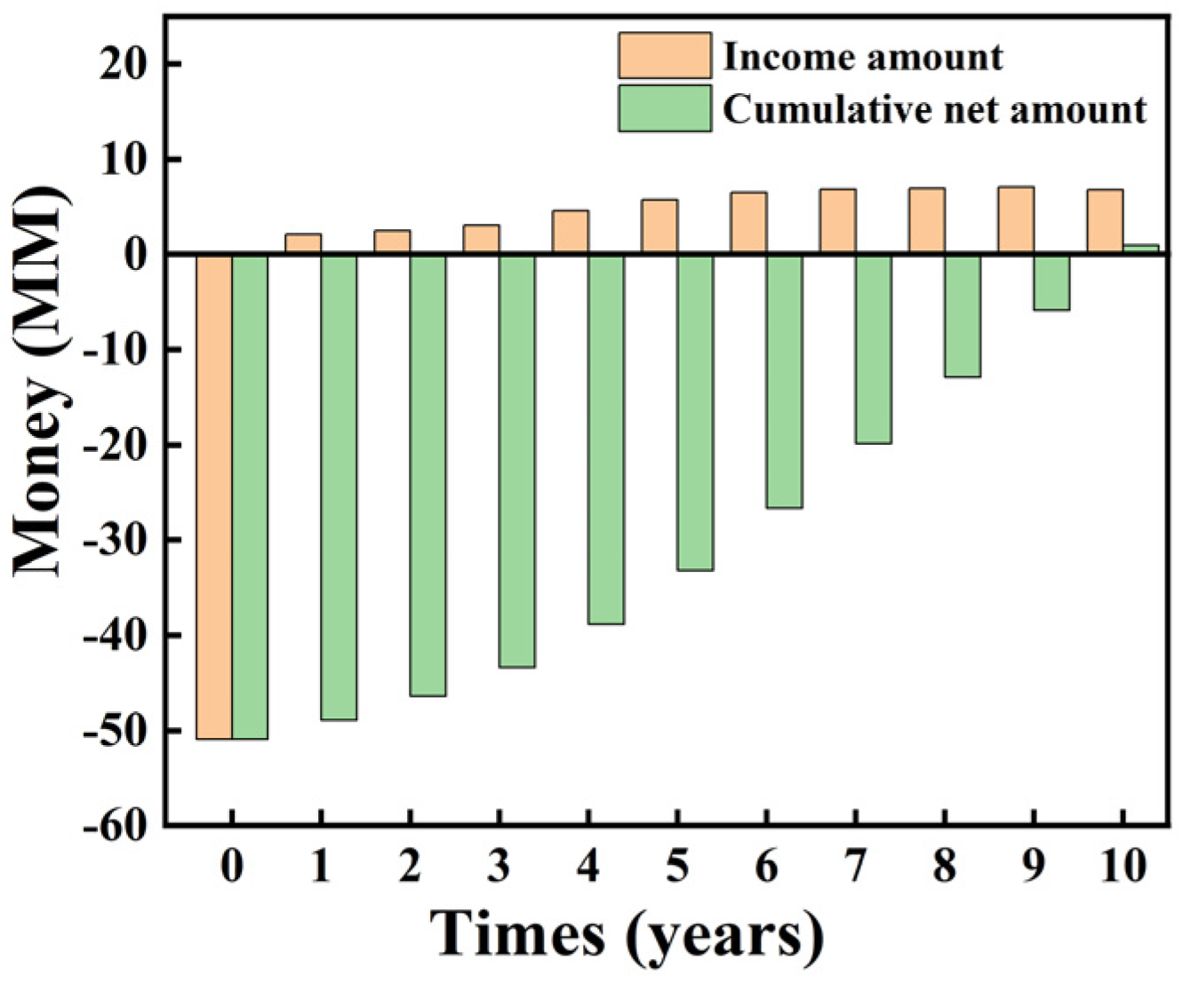
2.1.3. Economic Viability

To validate the feasibility of the system operating with different energy structures, two crucial economic parameters are introduced: net present value (NPV) and internal rate of return (IRR).

NPV refers to the difference between the discounted value of future cash flows generated by an energy structure investment and the project’s investment cost. When NPV > 0, it indicates that the energy structure can yield profits while meeting the benchmark rate of return. The calculation formula for NPV is as follows:

$$NPV={\displaystyle \sum }_{i=1}^n\frac{C{F}_i}{{\left(1+r\right)}^i}-C{F}_0$$

(29)

where $C{F}_i$ is cash inflows for each period, $C{F}_0$ is the initial capital investment, and $r$ is the periodic interest rate.

IRR is a closely related concept to NPV and refers to the discount rate at which the total present value of cash inflows equals the total present value of cash outflows, resulting in a net present value of zero. The calculation formula for IRR is as follows:

$${\displaystyle \sum }_{i=1}^n\frac{C{F}_i}{{\left(1+IRR\right)}^i}=C{F}_0$$

(30)

The economic evaluation of the system’s energy structure is conducted using the IRR. When the IRR exceeds the current discount rate, the NPV of the energy structure becomes greater than zero, indicating the feasibility of this energy structure. Conversely, if the IRR falls below the current discount rate, the energy structure is considered unfeasible. The economic feasibility of the energy structure is assessed by calculating both pre-tax and post-tax values through system operation.

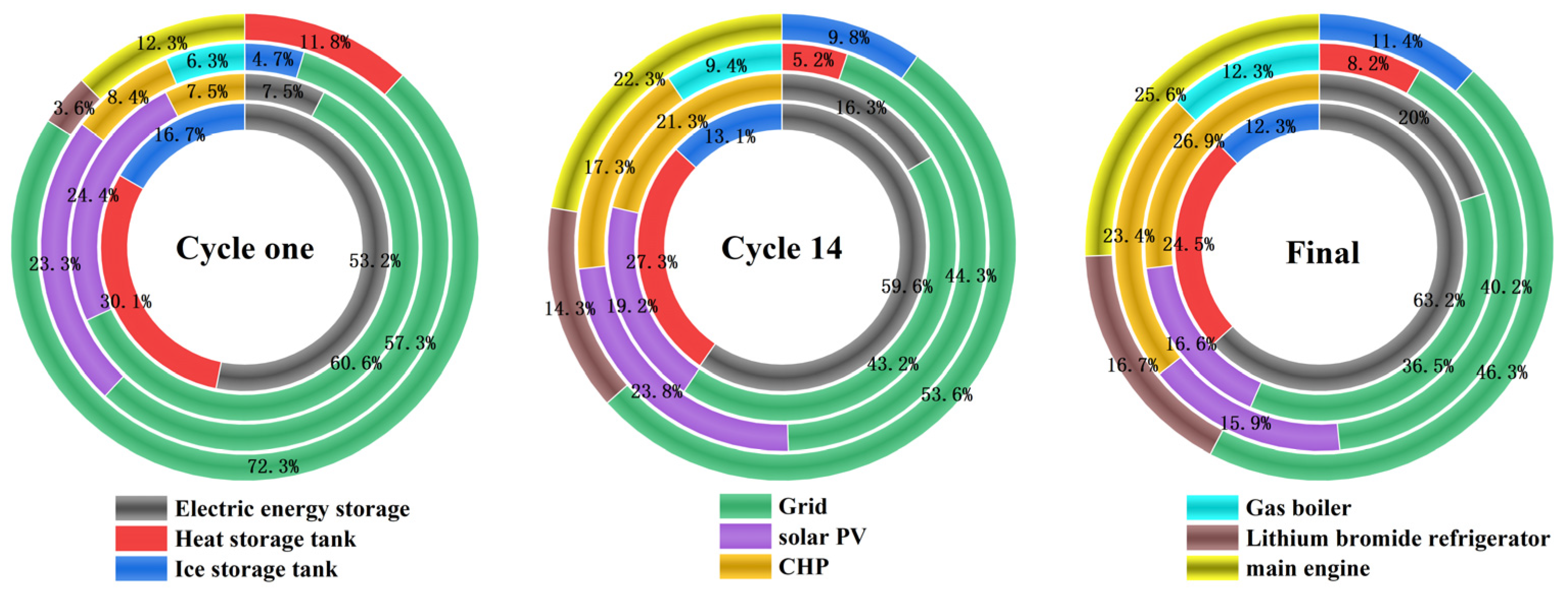
2.1.4. Energy and Component Cycle Optimization Method

In the optimization design and operation of integrated energy systems, the energy and component cycle (ECC) optimization method will be employed, coupled with scenario simulations. Scenario simulations utilize data related to energy structure and component parameters, combined with functions within neural networks, to perform simulations using data derived from daily scenario models. It enables the calculation of real-time data on component operation, energy consumption, and energy conservation effects. Scenario simulations over a single cycle are used to describe the uncertainty of energy demand and energy resources in an integrated energy system. Additionally, random system disturbances are introduced to simulate special circumstances that may occur in real-world situations. The ECC optimization method uses component capacity, power, and energy attributes as variables, with the ultimate goals of minimizing the total energy consumption ($Q_{total}$), total energy cost ($C_{total}$), and total carbon emissions ($E_{total}$) and ensuring the economic feasibility of the energy structure.

By generating random scenario data over cycles through simulation, this method is employed to evaluate and optimize system design solutions. The optimization process is continually refined on a per-cycle basis, ultimately yielding real-time simulation data, energy savings, and economic feasibility for the energy structure. This process involves eight main steps:

• Define decision variables. The primary decision variables in this approach encompass component parameters and energy attributes.
• Establish operating cycles. Following the scenario simulation method, determine the total operating duration and operating cycles to assess the initial design solution set periodically.
• Configure optimization scheme parameters based on the decision variables and operational cycles; set optimization scheme parameters.
• Simulate real-time operations. Utilizing component capacities, energy attributes, and operational cycles defined in the initial design solutions, simulate the operational states and power profiles of each component to meet the energy demands and constraints of the current real-time scenario.
• Compute scheme performance. Based on the real-time scenario simulation results, calculate the power profiles of various components, total energy cost, total carbon emissions, and total energy consumption over the operational cycle.
• Evaluate schemes. Assess the optimization and improvements needed for the current operational cycle based on the performance from the simulation.
• Determine the termination conditions. If the simulated runtime reaches the predefined operational time, exit the ECC optimization method and output all the result data. Otherwise, continue with step 8.
• Update optimization schemes. According to the results of the simulation and evaluation, retain certain optimization schemes within the collection and remove others to accommodate new optimization methods. Then, return to step 4 to continue the cycle simulation.

2.2. Case Study

In the case study, the integrated energy system architecture constructed is illustrated in Figure 1. The system includes the power grid, natural gas station, photovoltaic power plant, CHP, gas boiler, lithium bromide absorption chiller, airborne main engines, double-working condition main engines, energy storage battery, thermal storage tank, and ice storage tank. The electricity from the power grid and natural gas are considered as specific costs and energy expenditures in the system to meet the energy demands of residential and industrial sectors within a specific time. These demands primarily include the electrical power demands for lighting, air conditioning, computers, and other appliances in the area, as well as the heat demands for heating systems and water heaters and the cooling demands for air conditioning and refrigeration systems.

In this case study,

Table 1. Range of equipment capacities and investment costs per unit capacity.

Item (Unit)	Maximum Capacity	Minimum Capacity	Annual Price
Photovoltaic (kW)	80	0	50 USD/kw
CHP (kW)	600	0	40 USD/kw
Gas boiler (kW)	1200	0	6 USD/kw
Lithium bromide refrigerator (kW)	1000	0	15 USD/kw
Double-working condition main engine (kW)	900	0	17 USD/kw
Airborne main engine (kW)	300	0	15 USD/kw
Electric energy storage (kWh)	1500	0	20 USD/kwh
Heat storage tank (m3)	50	0	170 USD/m3
Ice storage tank (m3)	50	0	170 USD/m3

presents the capacity ranges and prices of various selected components [25,26].

Table 2. Fundamental parameters for electricity and natural gas.

Item	Price (USD/kWh)	Emission Factor (kg/kWh)	Consumption Factor (kWh/kWh)	Energy Purchase Tax Rate (%)
Power grid electricity	0.04/0.09/0.15	0.78	1.00	13
Natural gas	0.04	0.22	1.00	9

provides the energy, economic, and emissions attributes of the electricity grid and natural gas sources determined based on the chosen location in this case. Finally,

Table 3. System economic parameters.

Item (Unit)	Value
Capital ratio (%)	45
Lending rate (%)	3
Repayment period (year)	4
Surtax rate (%)	0.1
Income tax rate (%)	25
Benchmark return rate (%)	12
Facility deduction tax rate (%)	1
Equipment depreciation year (year)	3

summarizes the key economic parameters of this case [27]. Specific parameters are also established for special components in this case, such as energy storage components specially set the maximum number of charging energy cycles, capacity decay expressions, and input conversion to storage energy decay expression.

In this case, the ECC optimization method and real-time scheduling data are all solved using an improved genetic algorithm.

Table 4. System optimization parameters.

Item (Unit)	Value
Runtime (h)	8760
Run optimized population size	20
Run optimization iterations	25
Mutation operator	1.8
Cross operator	0.62

presents the common basic parameters of this algorithm. For stochastic optimization methods, the termination condition of the algorithm is to run optimization iterations, which involves setting a runtime for periodic simulation calculations. The algorithm outputs real-time scheduling data for energy devices, IRR, NPV, payback period, economic feasibility data, and energy conservation and emission reduction data from the last iteration to predict the feasibility of the energy structure.

3. Results and Discussion

3.1. Real-Time Scheduling Data

The system will provide real-time scheduling data for cases, which differ from conventional scheduling data. It is based on long-term evaluated parameters and takes into account the power related to the total energy consumption, carbon emissions, and energy costs of each component due to their operating time. Therefore, short-term overall scheduling plans are not considered, and long-term operational scheduling optimization is employed. Within the operating time of the energy structure, an optimized operational plan for the energy structure over a long period and multiple cycles is created by displaying real-time loads of various energy components in the aforementioned real-time scheduling data and combining them with the attributes of capacity and power of the components.

In this case study, the final energy demands of the energy structure are categorized into electricity, heating, and cooling requirements, with load curves for electricity, heating, and cooling being provided on an hourly basis. Figure 2 displays the real-time power of each energy component within one operating cycle for electric, heating, and cooling energy loads. By analyzing the variations in the long-term load rates of energy components, the energy utilization methods are continuously optimized based on the previous cycle’s operation. This ensures the comprehensive optimization of the energy structure’s generation, storage, and supply operation states in each operating cycle.

Figure 3 presents the distribution of the load proportions in this case study across three optimization cycles. The first circle from the inside out represents the energy storage proportions for the three major storage components, namely electricity, heat, and cold. Moving outward, the proportions indicate the energy interaction ratios for each component under electrical, thermal, and refrigeration loads, respectively. A comparison of the three operational cycles reveals that the proportion of electricity storage is significantly higher than that of heat and refrigeration storage. There are two reasons for this: first, the efficiency of refrigeration and heat storage is much lower than that of electricity storage; second, by utilizing electricity storage, excess power can be transferred and stored during periods of low electricity prices and sold or used as a backup power source during periods of high electricity prices. To reduce energy and grid costs, the system improves energy dispatch by deliberately reducing refrigeration and heat storage while increasing electricity storage in this energy structure. As the case study progresses, the utilization of CHP and gas boilers gradually increases. This is primarily due to the implementation of time-of-use electricity pricing, where the increased use of natural gas replaces electricity from the high-priced grid, thereby reducing costs and emissions. As the overall efficiency of CHP is higher than that of gas boilers, the quantity of gas boilers used is smaller than that of CHP.

3.2. Energy Conservation and Emission Reduction

Figure 4 shows the energy saving and emission reduction data under different optimization cycles.

Table 5. Energy saving and emission reduction in different cycle stages.

Optimization Period	Carbon Emission Reduction of the System/t	Other Emission Gas Reduction of the System/t	Proportion/%
1~5	91.90	30.19	11.07%
6~10	162.28	53.30	19.55%
11~15	185.15	60.82	22.30%
16~20	193.11	63.43	23.26%
21~25	197.74	64.91	23.82%

presents the proportion of energy saving and emission reduction during each cycle phase. Under the overall optimization period, the emission reductions of CO, CO₂, SO₂, NO_X, and PM_2.5 are 226.6, 830.5, 25.0, 12.5, and 8.3 tons. These reductions can be equivalently translated into the planting of 833,010 trees. The data indicate that the system, driven by electricity and natural gas as energy sources, can effectively achieve energy saving and emission reduction through multiple cycle optimizations, with significant initial optimization results.

3.3. Economic Feasibility

Figure 5 illustrates the projected capital recovery period for the system within the energy structure of this case study. The year 0 represents the total investment during the construction phase. Through the iterative optimization method applied to the one-year operational scenario, it can be inferred that the capital will be fully recovered within ten years, achieving initial profitability for the case. This further validates the economic feasibility of this case.

Table 6. Economic data output of the system.

Item (Unit)	Value
Total investment cost (million)	509.40
Pre-tax IRR (%)	23.14
Post-tax IRR (%)	21.96
Pre-tax NPV (million)	66.38
Post-tax NPV (million)	59.27

presents the economic parameters of the energy structure for this case over one project cycle (20 years). The pre-tax and post-tax IRR are 23.14% and 21.96%, respectively. These values significantly exceed the global inflation rate of 8.8% in 2022, and the International Monetary Fund (IMF) forecasted a global inflation rate of 6.5% for 2023, indicating that the energy structure of this case holds substantial investment value. The pre-tax and post-tax NPV are 66.38 and 59.27 million, respectively. The results demonstrate that the energy structure of this case, under current energy economic and environmental competitiveness, can maximize economic benefits while meeting energy conservation and emission reduction constraints.

The case study results reveal that utilizing renewable energy in the energy structure is highly worthwhile, primarily due to significantly reduced energy costs and superior energy conservation and emission reduction effects compared to traditional energy systems. However, the additional investments required for renewable energy technology, as well as ongoing technological advancements in this field, will lead to increased investment and maintenance costs for renewable energy systems.

4. Conclusions

This study presents a long-term, multi-period energy and component cycling optimization method based on genetic algorithms and deep learning. It dynamically utilizes various energy emission factors, price parameters, and the capacity flexibility of devices to integrate energy storage properties and peak–valley electricity attributes in real time. This optimization aims to align real-time energy dispatch objectives with long-term operational goals, with energy conservation and carbon reduction as the ultimate optimization objectives. The results and findings from this research are outlined as follows:

• The energy and component cycling optimization method proposed in this paper, considering the capacity of energy devices and loads, can effectively reduce costs and carbon emissions.
• Conducting an economic feasibility assessment on the integrated energy system enables more efficient prediction and evaluation of whether the system is worth investing in and operating.
• By appropriately increasing the usage of pricing clean energy sources such as natural gas in the integrated energy system to offset the use of expensive peak–valley electricity, while reducing the capacity and load scheduling of thermal and cooling storage devices, the system’s operational efficiency can be significantly improved.

References

1. Bilgen, S. Structure and environmental impact of global energy consumption. Renew. Sustain. Energy Rev. 2014, 38, 890–902. [Google Scholar] [CrossRef]
2. Armaroli, N.; Balzani, V. The future of energy supply: Challenges and opportunities. Angew. Chem. Int. Ed. 2007, 46, 52–66. [Google Scholar] [CrossRef] [PubMed]
3. Kaundinya, D.P.; Balachandra, P.; Ravindranath, N.H. Grid-connected versus stand-alone energy systems for decentralized power—A review of literature. Renew. Sustain. Energy Rev. 2009, 13, 2041–2050. [Google Scholar] [CrossRef]
4. Gielen, D.; Boshell, F.; Saygin, D.; Bazilian, M.D.; Wagner, N.; Gorini, R. The role of renewable energy in the global energy transformation. Energy Strategy Rev. 2019, 24, 38–50. [Google Scholar] [CrossRef]
5. Qin, C.; Yan, Q.; He, G. Integrated energy systems planning with electricity, heat and gas using particle swarm optimization. Energy 2019, 188, 116044. [Google Scholar] [CrossRef]
6. Ringkjøb, H.K.; Haugan, P.M.; Solbrekke, I.M. A review of modelling tools for energy and electricity systems with large shares of variable renewables. Renew. Sustain. Energy Rev. 2018, 96, 440–459. [Google Scholar] [CrossRef]
7. Nie, X.; Daud, W.S.A.W.M.; Pu, J. A novel transactive integration system for solar renewable energy into smart homes and landscape design: A digital twin simulation case study. Sol. Energy 2023, 262, 111871. [Google Scholar] [CrossRef]
8. Wang, J.; El Kontar, R.; Jin, X.; King, J. Electrifying high-efficiency future communities: Impact on energy, emissions, and grid. Adv. Appl. Energy 2022, 6, 100095. [Google Scholar] [CrossRef]
9. Wang, Y.; Qin, Y.; Ma, Z.; Wang, Y.; Li, Y. Operation optimisation of integrated energy systems based on cooperative game with hydrogen energy storage systems. Int. J. Hydrogen Energy 2023, 48, 37335–37354. [Google Scholar] [CrossRef]
10. Naili, N.; Kooli, S. Solar-assisted ground source heat pump system operated in heating mode: A case study in Tunisia. Renew. Sustain. Energy Rev. 2021, 145, 111144. [Google Scholar] [CrossRef]
11. Favre-Perrod, P. A vision of future energy networks. In Proceedings of the 2005 IEEE Power Engineering Society Inaugural Conference and Exposition in Africa, Durban, South Africa, 11–15 July 2005; pp. 13–17. [Google Scholar]
12. Revesz, A.; Jones, P.; Dunham, C.; Davies, G.; Marques, C.; Matabuena, R.; Scott, J.; Maidment, G. Developing novel 5th generation district energy networks. Energy 2020, 201, 117389. [Google Scholar] [CrossRef]
13. Geidl, M. Integrated Modeling and Optimization of Multi-Carrier Energy Systems; ETH Zurich: Zurich, Switzerland, 2007. [Google Scholar]
14. Kazemdehdashti, A.; Mohammadi, M.; Seifi, A.R.; Rastegar, M. Stochastic energy management in multi-carrier residential energy systems. Energy 2020, 202, 117790. [Google Scholar] [CrossRef]
15. Yin, L.; Wu, Y. Deep Stackelberg heuristic dynamic programming for frequency regulation of interconnected power systems considering flexible energy sources. Eng. Appl. Artif. Intell. 2021, 106, 104508. [Google Scholar] [CrossRef]
16. Turk, A.; Wu, Q.; Zhang, M.; Østergaard, J. Day-ahead stochastic scheduling of integrated multi-energy system for flexibility synergy and uncertainty balancing. Energy 2020, 196, 117130. [Google Scholar] [CrossRef]
17. Hilpert, S.; Kaldemeyer, C.; Krien, U.; Günther, S.; Wingenbach, C.; Plessmann, G. The Open Energy Modelling Framework (oemof)—A new approach to facilitate open science in energy system modelling. Energy Strategy Rev. 2018, 22, 16–25. [Google Scholar] [CrossRef]
18. Lopion, P.; Markewitz, P.; Robinius, M.; Stolten, D. A review of current challenges and trends in energy systems modeling. Renew. Sustain. Energy Rev. 2018, 96, 156–166. [Google Scholar] [CrossRef]
19. Tonellato, G.; Heidari, A.; Pereira, J.; Carnieletto, L.; Flourentzou, F.; De Carli, M.; Khovalyg, D. Optimal design and operation of a building energy hub: A comparison of exergy-based and energy-based optimization in Swiss and Italian case studies. Energy Convers. Manag. 2021, 242, 114316. [Google Scholar] [CrossRef]
20. Miglani, S.; Orehounig, K.; Carmeliet, J. Integrating a thermal model of ground source heat pumps and solar regeneration within building energy system optimization. Appl. Energy 2018, 218, 78–94. [Google Scholar] [CrossRef]
21. Jin, B.; Song, J.; Liao, Y. Comparative study on the improvement of a distributed energy system performance by optimized operation strategy from design to operation. Energy Rep. 2023, 10, 1726–1738. [Google Scholar] [CrossRef]
22. Song, X.T.; Sun, Y.; Liu, X.B.; Zhou, J.H.; Li, W.B. Multi-objective bilevel programming strategy of integrated energy system considering regional interconnection[J/OL]. High Volt. Technol. 2023, 1–16. [Google Scholar]
23. Liu, Y.Y.; Wang, L.; Kun, W. Research on integrated energy cycle operation control strategy based on multiobjective optimization algorithm. Electron. Des. Eng. 2023, 31, 98–102. [Google Scholar]
24. Zhang, Z.H.; Zhang, Z.Y.; Zhang, X.J.; Pang, G.Z. Optimal operation regulation strategy of multi-energy complementary system considering source load storage dynamic characteristics in oilfield well sites. Electr. Power Syst. Res. 2023, 225, 109799. [Google Scholar] [CrossRef]
25. Li, H.; Zhang, C.; Sun, B. Optimal design and operation method of integrated energy system based on stochastic scenario iteration and energy storage attribute evaluation. Sustain. Cities Soc. 2023, 95, 104585. [Google Scholar] [CrossRef]
26. Pan, C.; Fan, G.; Wang, J.; Xu, X.; Meng, T. Low-Carbon Optimization of Electric and Heating Integrated Energy System with Flexible Resource Participation. J. Electrotech. Technol. 2023, 38, 1633–1647. [Google Scholar]
27. Foslie, S.S.; Knudsen, B.R.; Korpås, M. Integrated design and operational optimization of energy systems in dairies. Energy 2023, 281, 128242. [Google Scholar] [CrossRef]
Figure 1. Schematic representation of the case. (In the figure, yellow lines represent electricity, green represents natural gas, red represents heat load and blue represents cold load).
Algorithms 16 00530 g001
Figure 2. Load profiles of various energy components within one operating cycle. ((a) represents the power load curve of each energy equipment in a period; (b) represents the heat load curve of each energy equipment in a period; (c) represents the cold load curve of each energy equipment in a period).
Algorithms 16 00530 g002
Figure 3. Energy ratio diagram under three different operating cycles.
Algorithms 16 00530 g003
Figure 4. Energy saving and emission reduction curve in each optimization period.
Algorithms 16 00530 g004
Figure 5. Cost recovery projection chart.
Algorithms 16 00530 g005