
On the Intersection of Computational Geometry Algorithms with Mobile Robot Path Planning

Abstract
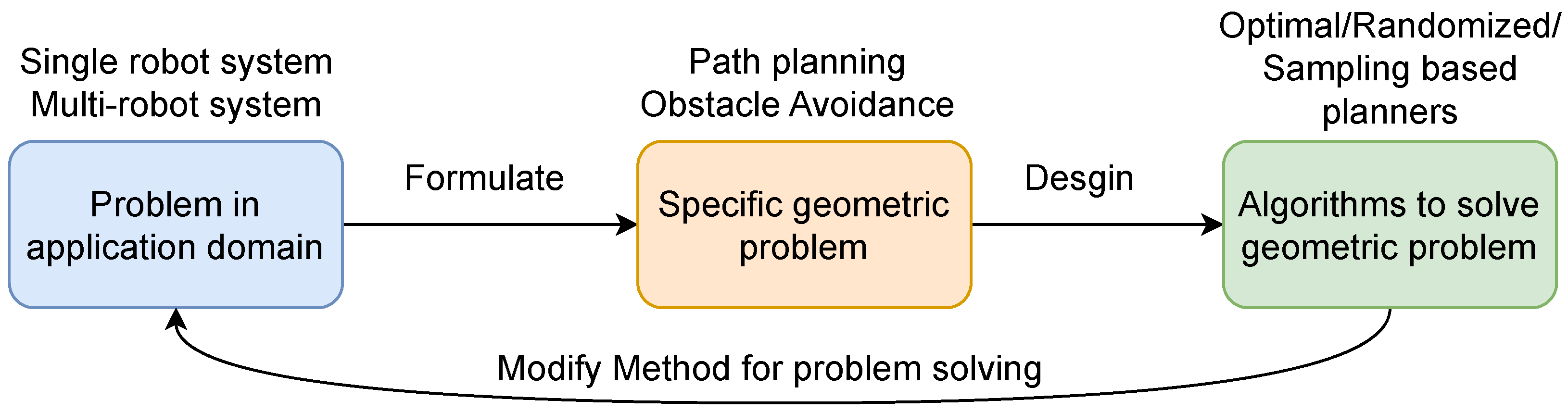
:1. Introduction
- First, the scope of path planning is clearly demarcated into two primary areas: single-robot and multi-robot systems;
- The review predominantly focuses on the literature published between 2016 and 2023, considering papers using CG in mobile robots, ensuring relevance and incorporation of the latest advancements in the field; however, to discuss the foundational work on computational geometry, we have considered pioneering works from the years 1969 to 2008;
- We also have taken articles from the winners of CG-SHOP 2021, as they are the most relevant and recent works on the discussed topic;
- During the literature search, keywords such as “computational geometry in robot path planning”, “single-robot path planning”, “multi-robot coordination”, and “kino-dynamic path planning” were employed. These were searched across renowned databases like IEEE Xplore, Google Scholar, and ScienceDirect;
- Subsequently, the selected literature was examined based on specific criteria such as relevance to the topic, citation count, and the novelty of the proposed solutions;
- The extracted information was then organized and synthesized to offer a comparative analysis, using features such as algorithmic complexity, optimality, scalability, and real-world applicability for comparing various solutions.
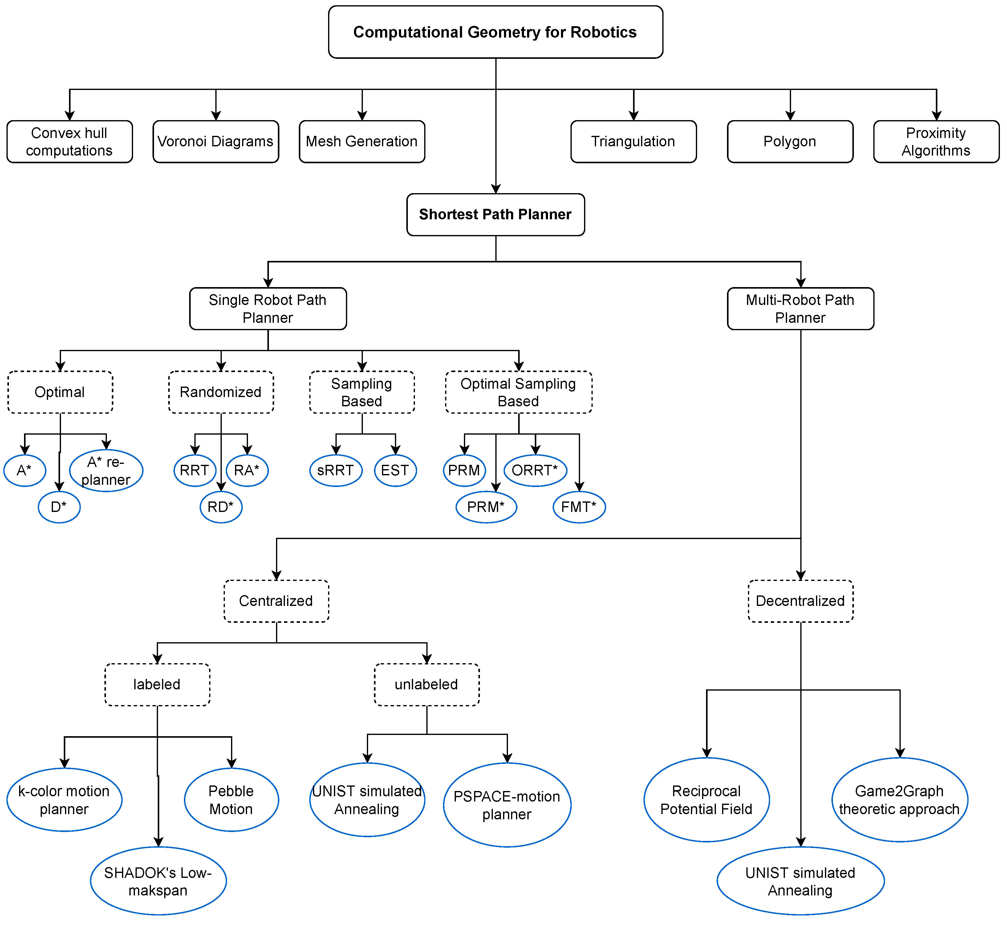
1.1. Computational Geometry
- Bézier, Forrest, and Riesenfeld have successfully handled the problem of geometric modeling using spline curves and surfaces [7], which is more closely related to numerical analysis than geometry in terms of spirit;
- Many computer scientists believe that Michael Shamos’ Ph.D. thesis at Yale University in 1978 [8] or perhaps his earlier paper on geometric complexity [9] are the two works that gave rise to the field of computational geometry, which is frequently referred to as a new one in the area of computing science;
- Finally, others would argue that the formal examination of Minsky and Papert [11] into which geometric properties of a figure can and cannot be identified (computed) using different neural network models of computation is where it all started.
- Size of input to the algorithm;
- Dimension of the problem;
- Properly defined constraints;
- Objective functions;
- Modality of the algorithm.
1.2. Robotics
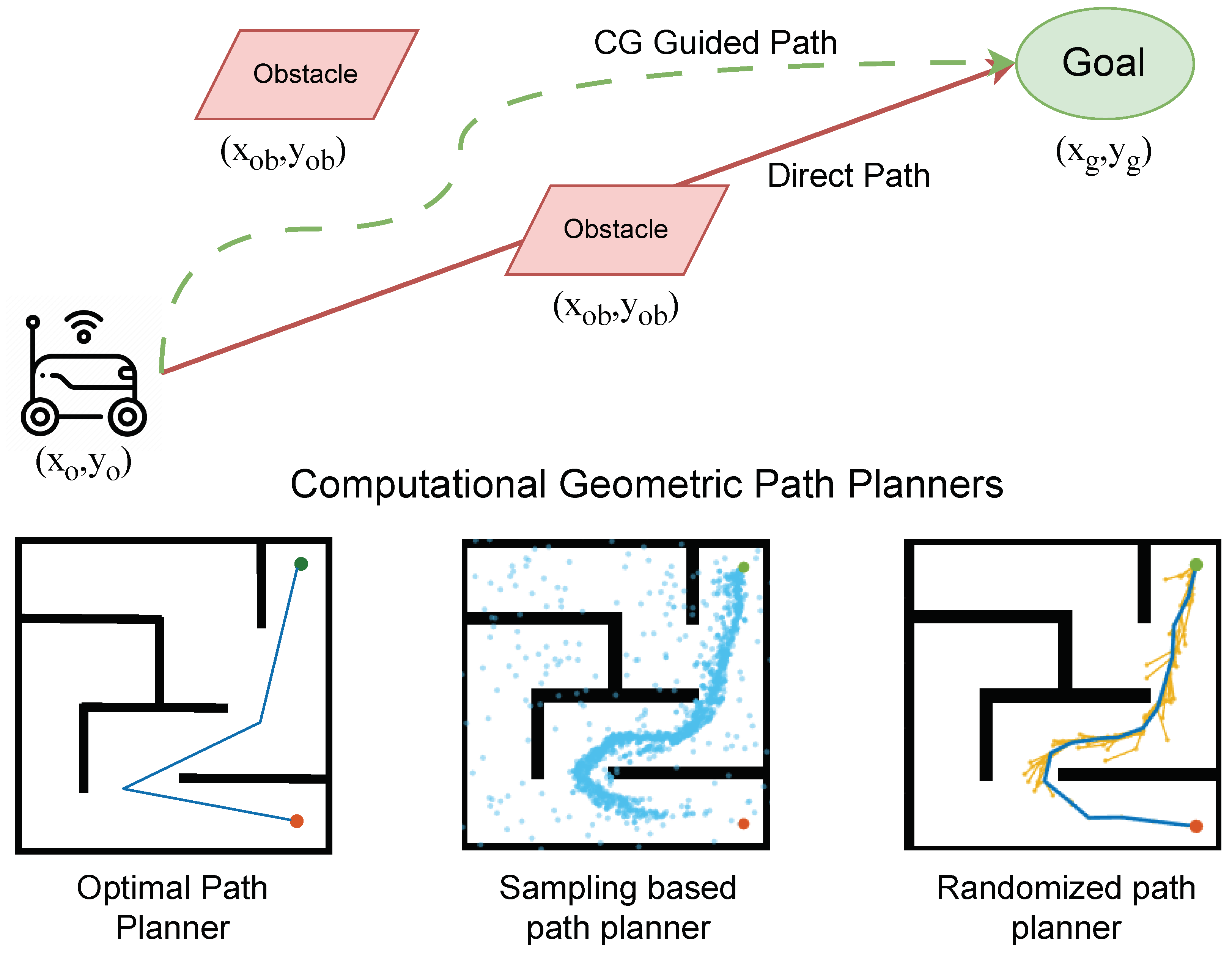
2. Path Planning
2.1. CG-Based Single-Robot Path Planning
- Select a random sample from C;
- Determine a region R in C such that the probability of selecting a sample from R is inversely proportional to the volume of C already explored by T in R;
- If lies in R, attempt to connect to the nearest node in the tree T;
- Add to T if a valid connection is established.
- For to n, sample a configuration from C;
- If is collision-free, add it to V;
- For each , attempt to connect q to k nearest neighbors in V that are collision-free;
- Add valid connections to E.
- Sample a random configuration from C;
- Find the nearest node in T to ;
- Attempt to connect to T through , resulting in ;
- If the connection is valid, look for nodes in T within a radius r of and attempt to rewire the tree to minimize the path cost.
2.2. Transitioning from a Single-Robot to Multi-Robot Path Planning
- Inter-Robot Collisions: Unlike the single-robot scenario, the risk of collisions is not limited to static obstacles. Dynamic collisions between robots present a substantial challenge. The movement of one robot might obstruct the path of another, necessitating continuous reevaluation and adaptation;
- Coordinated Movement: Ensuring that all robots reach their respective destinations within optimal time frames demands a high degree of coordination. This often involves sacrificing individual robot efficiency for collective efficiency;
- Increased Configuration Complexity: The configuration space exponentially grows with the addition of each robot. This expansion augments the computational overhead and complicates the search for optimal paths.
- Minkowski Sum [25]: This can be employed to compute the configuration space obstacles when dealing with moving robots. By considering one robot as the primary agent and treating other robots as moving obstacles, the problem can be reduced to a single-robot scenario in an augmented environment;
- Voronoi Diagrams [26]: These can assist in partitioning the workspace, providing each robot with a distinct region to navigate. This ensures a degree of separation between the robots, minimizing potential collisions;
- Visibility Graphs [27]: For environments with multiple robots and obstacles, visibility graphs can be extended to incorporate dynamic inter-robot constraints. This ensures that, while navigating from source to destination, the robot considers both static and dynamic elements in its path.
2.3. Multi-Robot Path Planning
| Algorithm 1 Generalized Algorithmic Overview for Multi-Robot Path Planning |
|

| Algorithm | Category | Best Case | Worst Case | Average Case | Optimality | Update Cost | Abbreviations |
|---|---|---|---|---|---|---|---|
| Labeled [30] | Centralized | complete | low | b—no. of obstacles, m—no. of robots, n—no. of cells | |||
| Unlabeled [32] | Centralized | complete | low | n—number of cells | |||
| Reciprocal [33] | Decentralized | - | sub | high | —makespan factor | ||
| Game-theoretic [34] | Decentralized | - | sub | high | —depth factor | ||
| Shadok [35] | Distributed | - | sub | high | w—number of labeled units | ||
| UNIST [28] | Distributed | - | sub | high | w—maximum space dimension | ||
| Gitastrophe k-opt [29] | Distributed | - | complete | moderate | k—number of robots and w—number of squares |
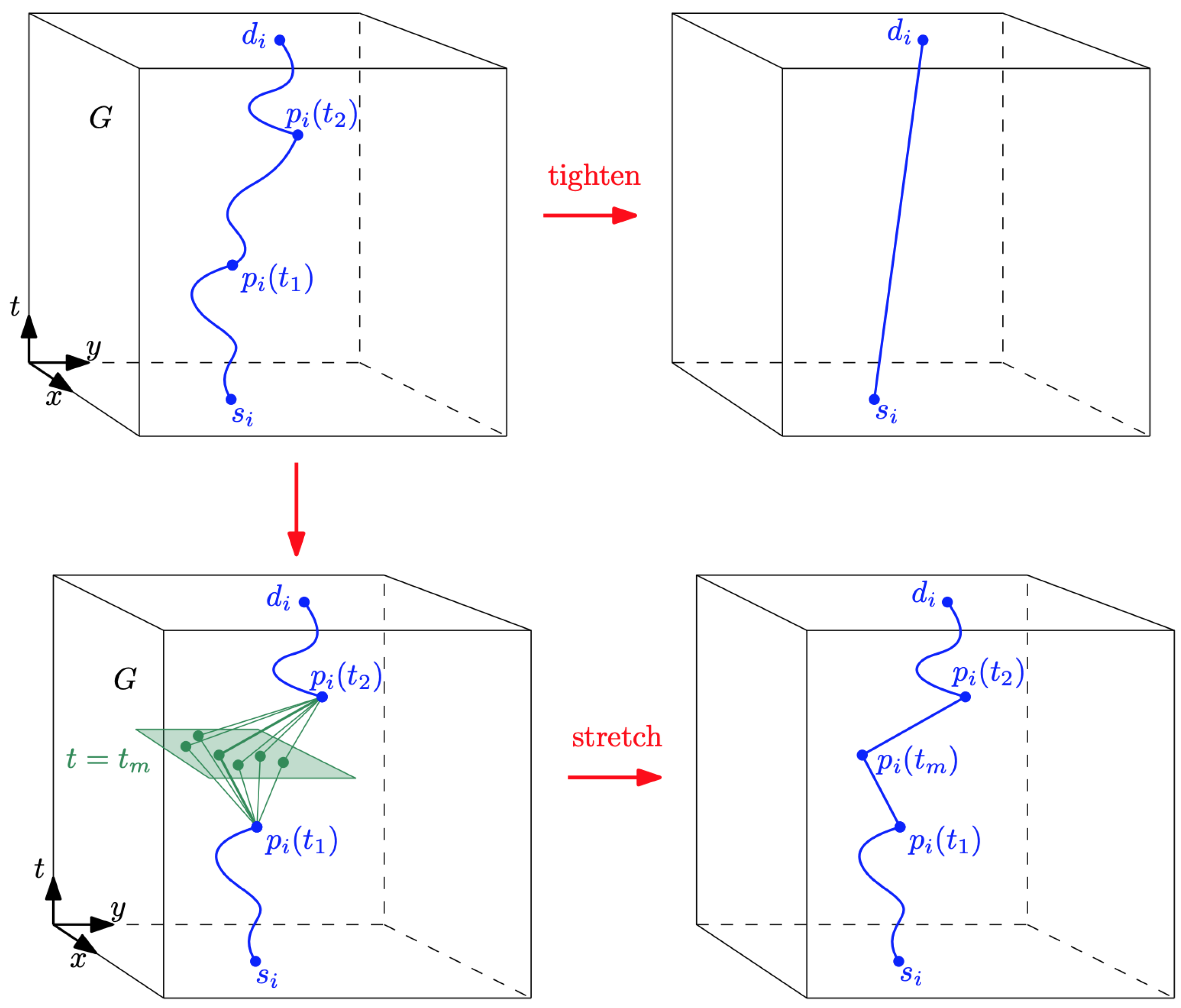
2.4. Distributed Approaches from CG-SHOP 2021
3. Future Directions
4. Conclusions
Author Contributions
Funding
Data Availability Statement
Conflicts of Interest
Abbreviations
| CG | Computational Geometry |
| PRM | Probabilistic Road Map |
| DFS | Depth First Search |
| RRT | Rapidly-exploring Random Tree |
| EST | Expansive-Space Tree |
| FM | Fast Marching |
References
- Mark, D.B.; Otfried, C.; Marc, V.K.; Mark, O. Computational Geometry Algorithms and Applications; Spinger: Berlin/Heidelberg, Germany, 2008. [Google Scholar]
- Berg, M.D.; Kreveld, M.V.; Overmars, M.; Schwarzkopf, O. Computational geometry. In Computational Geometry; Springer: Berlin/Heidelberg, Germany, 1997; pp. 1–17. [Google Scholar]
- Preparata, F.P.; Shamos, M.I. Computational Geometry: An Introduction; Springer Science & Business Media: Berlin/Heidelberg, Germany, 2012. [Google Scholar]
- Forrest, A.R. Computational geometry-achievements and problems. In Computer Aided Geometric Design; Elsevier: Amsterdam, The Netherlands, 1974; pp. 17–44. [Google Scholar]
- Riesenfeld, R.F. Applications of b-Spline Approximation to Geometric Problems of Computer-Aided Design; Syracuse University: Syracuse, NY, USA, 1973. [Google Scholar]
- Lee, D.T.; Preparata, F.P. Computational geometry: A survey. IEEE Trans. Comput. 1984, 33, 1072–1101. [Google Scholar] [CrossRef]
- Gordon, W.J.; Riesenfeld, R.F. B-spline curves and surfaces. In Computer Aided Geometric Design; Elsevier: Amsterdam, The Netherlands, 1974; pp. 95–126. [Google Scholar]
- Shamos, M.I. Computational Geometry; Yale University: New Haven, CT, USA, 1978. [Google Scholar]
- Shamos, M.I. Geometric complexity. In Proceedings of the Seventh Annual ACM Symposium on Theory of Computing, Albuquerque, NM, USA, 5–7 May 1975; pp. 224–233. [Google Scholar]
- Forrest, A.R. Curves and Surfaces for Computer-Aided Design. Ph.D. Thesis, University of Cambridge, Cambridge, UK, 1968. [Google Scholar]
- Minsky, M.; Papert, S. Perceptron: An Introduction to Computational Geometry; MIT Press: Cambridge, MA, USA, 1969. [Google Scholar]
- Knoblauch, J.; Husain, H.; Diethe, T. Optimal continual learning has perfect memory and is np-hard. In Proceedings of the International Conference on Machine Learning, PMLR 2020, Virtual, 13–18 July 2020; pp. 5327–5337. [Google Scholar]
- Campbell, S.; O’Mahony, N.; Carvalho, A.; Krpalkova, L.; Riordan, D.; Walsh, J. Path planning techniques for mobile robots a review. In Proceedings of the 2020 6th International Conference on Mechatronics and Robotics Engineering (ICMRE), Barcelona, Spain, 12–15 February 2020; pp. 12–16. [Google Scholar]
- Dudi, T.; Singhal, R.; Kumar, R. Shortest Path Evaluation with Enhanced Linear Graph and Dijkstra Algorithm. In Proceedings of the 2020 59th Annual Conference of the Society of Instrument and Control Engineers of Japan (SICE), Chiang Mai, Thailand, 23–26 September 2020; pp. 451–456. [Google Scholar]
- Patle, B.; Pandey, A.; Parhi, D.; Jagadeesh, A. A review: On path planning strategies for navigation of mobile robot. Def. Technol. 2019, 15, 582–606. [Google Scholar] [CrossRef]
- Pérez-Hurtado, I.; Martínez-del Amor, M.Á.; Zhang, G.; Neri, F.; Pérez-Jiménez, M.J. A membrane parallel rapidly-exploring random tree algorithm for robotic motion planning. Integr. Comput.-Aided Eng. 2020, 27, 121–138. [Google Scholar] [CrossRef]
- Ammar, A.; Bennaceur, H.; Châari, I.; Koubâa, A.; Alajlan, M. Relaxed Dijkstra and A* with linear complexity for robot path planning problems in large-scale grid environments. Soft Comput. 2016, 20, 4149–4171. [Google Scholar] [CrossRef]
- Arias, F.F.; Ichter, B.; Faust, A.; Amato, N.M. Avoidance critical probabilistic roadmaps for motion planning in dynamic environments. In Proceedings of the 2021 IEEE International Conference on Robotics and Automation (ICRA), Xi’an, China, 30 May–5 June 2021; pp. 10264–10270. [Google Scholar]
- Tahir, Z.; Qureshi, A.H.; Ayaz, Y.; Nawaz, R. Potentially guided bidirectionalized RRT* for fast optimal path planning in cluttered environments. Robot. Auton. Syst. 2018, 108, 13–27. [Google Scholar] [CrossRef]
- Varava, A.; Carvalho, J.F.; Pokorny, F.T.; Kragic, D. Caging and path non-existence: A deterministic sampling-based verification algorithm. In Robotics Research; Springer: Berlin/Heidelberg, Germany, 2020; pp. 589–604. [Google Scholar]
- Wang, Z.; Li, Y.; Zhang, H.; Liu, C.; Chen, Q. Sampling-based optimal motion planning with smart exploration and exploitation. IEEE/ASME Trans. Mechatron. 2020, 25, 2376–2386. [Google Scholar] [CrossRef]
- Solovey, K.; Salzman, O.; Halperin, D. New perspective on sampling-based motion planning via random geometric graphs. Int. J. Robot. Res. 2018, 37, 1117–1133. [Google Scholar] [CrossRef]
- Gammell, J.D.; Strub, M.P. Asymptotically optimal sampling-based motion planning methods. Annu. Rev. Control Robot. Auton. Syst. 2021, 4, 295–318. [Google Scholar] [CrossRef]
- Gao, F.; Wu, W.; Lin, Y.; Shen, S. Online safe trajectory generation for quadrotors using fast marching method and bernstein basis polynomial. In Proceedings of the 2018 IEEE International Conference on Robotics and Automation (ICRA), Brisbane, Australia, 21–25 May 2018; pp. 344–351. [Google Scholar]
- Adler, A.; Berg, M.D.; Halperin, D.; Solovey, K. Efficient multi-robot motion planning for unlabeled discs in simple polygons. In Algorithmic Foundations of Robotics XI; Springer: Berlin/Heidelberg, Germany, 2015; pp. 1–17. [Google Scholar]
- Huang, S.K.; Wang, W.J.; Sun, C.H. A path planning strategy for multi-robot moving with path-priority order based on a generalized Voronoi diagram. Appl. Sci. 2021, 11, 9650. [Google Scholar] [CrossRef]
- Blasi, L.; D’Amato, E.; Mattei, M.; Notaro, I. Path planning and real-time collision avoidance based on the essential visibility graph. Appl. Sci. 2020, 10, 5613. [Google Scholar] [CrossRef]
- Yang, H.; Vigneron, A. A Simulated Annealing Approach to Coordinated Motion Planning (CG Challenge). In Proceedings of the 37th International Symposium on Computational Geometry (SoCG 2021), Buffalo, NY, USA, 7–11 June 2021. [Google Scholar]
- Liu, P.; Spalding-Jamieson, J.; Zhang, B.; Zheng, D.W. Coordinated motion planning through randomized k-opt. ACM J. Exp. Algorithmics (JEA) 2022, 27, 1–9. [Google Scholar] [CrossRef]
- Shome, R.; Solovey, K.; Dobson, A.; Halperin, D.; Bekris, K.E. drrt*: Scalable and informed asymptotically-optimal multi-robot motion planning. Auton. Robot. 2020, 44, 443–467. [Google Scholar] [CrossRef]
- Li, Q.; Gama, F.; Ribeiro, A.; Prorok, A. Graph neural networks for decentralized multi-robot path planning. In Proceedings of the 2020 IEEE/RSJ International Conference on Intelligent Robots and Systems (IROS), Las Vegas, NV, USA, 25–29 October 2020; pp. 11785–11792. [Google Scholar]
- Lurz, H.; Recker, T.; Raatz, A. Spline-based Path Planning and Reconfiguration for Rigid Multi-Robot Formations. Procedia CIRP 2022, 106, 174–179. [Google Scholar] [CrossRef]
- Bareiss, D.; Van den Berg, J. Generalized reciprocal collision avoidance. Int. J. Robot. Res. 2015, 34, 1501–1514. [Google Scholar] [CrossRef]
- Smyrnakis, M.; Qu, H.; Veres, S.M. Improving multi-robot coordination by game-theoretic learning algorithms. Int. J. Artif. Intell. Tools 2018, 27, 1860015. [Google Scholar] [CrossRef]
- Crombez, L.; da Fonseca, G.D.; Gerard, Y.; Gonzalez-Lorenzo, A.; Lafourcade, P.; Libralesso, L. Shadoks approach to low-makespan coordinated motion planning. ACM J. Exp. Algorithms (JEA) 2021, 27, 1–17. [Google Scholar] [CrossRef]
- Debord, M.; Hönig, W.; Ayanian, N. Trajectory planning for heterogeneous robot teams. In Proceedings of the 2018 IEEE/RSJ International Conference on Intelligent Robots and Systems (IROS), Madrid, Spain, 1–5 October 2018; pp. 7924–7931. [Google Scholar]
- Solovey, K.; Halperin, D. On the hardness of unlabeled multi-robot motion planning. Int. J. Robot. Res. 2016, 35, 1750–1759. [Google Scholar] [CrossRef]
- Bajcsy, A.; Herbert, S.L.; Fridovich-Keil, D.; Fisac, J.F.; Deglurkar, S.; Dragan, A.D.; Tomlin, C.J. A scalable framework for real-time multi-robot, multi-human collision avoidance. In Proceedings of the 2019 International Conference on Robotics and Automation (ICRA), Montreal, QC, Canada, 20–24 May 2019; pp. 936–943. [Google Scholar]
- Agarwal, P.K.; Geft, T.; Halperin, D.; Taylor, E. Multi-robot motion planning for unit discs with revolving areas. Comput. Geom. 2023, 114, 102019. [Google Scholar] [CrossRef]
- Şenbaşlar, B.; Sukhatme, G.S. Asynchronous Real-time Decentralized Multi-Robot Trajectory Planning. In Proceedings of the 2022 IEEE/RSJ International Conference on Intelligent Robots and Systems (IROS), Kyoto, Japan, 23–27 October 2022; pp. 9972–9979. [Google Scholar]
- Choi, C.; Adil, M.; Rahmani, A.; Madani, R. Multi-robot motion planning via parabolic relaxation. IEEE Robot. Autom. Lett. 2022, 7, 6423–6430. [Google Scholar] [CrossRef]
- Wang, X.; Sahin, A.; Bhattacharya, S. Coordination-free multi-robot path planning for congestion reduction using topological reasoning. J. Intell. Robot. Syst. 2023, 108, 50. [Google Scholar] [CrossRef]
- Zhang, H.; Chan, S.H.; Zhong, J.; Li, J.; Koenig, S.; Nikolaidis, S. A mip-based approach for multi-robot geometric task-and-motion planning. In Proceedings of the 2022 IEEE 18th International Conference on Automation Science and Engineering (CASE), Mexico City, Mexico, 22–26 August 2022; pp. 2102–2109. [Google Scholar]
- Fekete, S.P.; Keldenich, P.; Krupke, D.; Mitchell, J.S. Computing coordinated motion plans for robot swarms: The cg: Shop challenge 2021. ACM J. Exp. Algorithmics (JEA) 2022, 27, 1–12. [Google Scholar] [CrossRef]


Disclaimer/Publisher’s Note: The statements, opinions and data contained in all publications are solely those of the individual author(s) and contributor(s) and not of MDPI and/or the editor(s). MDPI and/or the editor(s) disclaim responsibility for any injury to people or property resulting from any ideas, methods, instructions or products referred to in the content. |
© 2023 by the authors. Licensee MDPI, Basel, Switzerland. This article is an open access article distributed under the terms and conditions of the Creative Commons Attribution (CC BY) license (https://creativecommons.org/licenses/by/4.0/).
Share and Cite
Latif, E.; Parasuraman, R. On the Intersection of Computational Geometry Algorithms with Mobile Robot Path Planning. Algorithms 2023, 16, 498. https://doi.org/10.3390/a16110498
Latif E, Parasuraman R. On the Intersection of Computational Geometry Algorithms with Mobile Robot Path Planning. Algorithms. 2023; 16(11):498. https://doi.org/10.3390/a16110498
Chicago/Turabian StyleLatif, Ehsan, and Ramviyas Parasuraman. 2023. "On the Intersection of Computational Geometry Algorithms with Mobile Robot Path Planning" Algorithms 16, no. 11: 498. https://doi.org/10.3390/a16110498
APA StyleLatif, E., & Parasuraman, R. (2023). On the Intersection of Computational Geometry Algorithms with Mobile Robot Path Planning. Algorithms, 16(11), 498. https://doi.org/10.3390/a16110498