Anomaly Detection for Skin Lesion Images Using Convolutional Neural Network and Injection of Handcrafted Features: A Method That Bypasses the Preprocessing of Dermoscopic Images

Abstract

Skin cancer (SC) is one of the most common cancers in the world and is a leading cause of death in humans. Melanoma (M) is the most aggressive form of skin cancer and has an increasing incidence rate. Early and accurate diagnosis of M is critical to increase patient survival rates; however, its clinical evaluation is limited by the long timelines, variety of interpretations, and difficulty in distinguishing it from nevi (N) because of striking similarities. To overcome these problems and to support dermatologists, several machine-learning (ML) and deep-learning (DL) approaches have been developed. In the proposed work, melanoma detection, understood as an anomaly detection task with respect to the normal condition consisting of nevi, is performed with the help of a convolutional neural network (CNN) along with the handcrafted texture features of the dermoscopic images as additional input in the training phase. The aim is to evaluate whether the preprocessing and segmentation steps of dermoscopic images can be bypassed while maintaining high classification performance. Network training is performed on the ISIC2018 and ISIC2019 datasets, from which only melanomas and nevi are considered. The proposed network is compared with the most widely used pre-trained networks in the field of dermatology and shows better results in terms of classification and computational cost. It is also tested on the ISIC2016 dataset to provide a comparison with the literature: it achieves high performance in terms of accuracy, sensitivity, and specificity.

1. Introduction

Skin cancer is one of the most common types of cancer in the global Caucasian population [1]. It is one of the three most dangerous and fastest-growing types of cancer and is therefore a serious public health problem [2]. Skin tumors can be benign [3] or malignant; the main malignant cancers are basalioma, squamous cell carcinoma, and malignant melanoma [4]. Of these, melanoma is the least common but at the same time is the most aggressive, and it can lead to death if diagnosed late. Therefore, it is critical to detect it early, which increases the chances of treatment and cure [5]. Its diagnosis follows some simple rules [6]: the ABCDE rule, which is based on morphological features of the lesions such as asymmetry (A), border irregularity (B), color variety (C), diameter (D), and evolution (E); the Seven Point Checklist, which is based on seven dermoscopic features representative of melanoma; and the Menzies method, which scores based on the presence/absence of certain positive or negative characteristics. The ABCDE rule is the most widely used because of the winning combination of ease of application and diagnostic efficacy. In fact, while nevi generally are symmetrical (round or oval), have regular edges (smooth and uniform), show homogeneous color, small size (diameter less than 6 mm), and do not evolve over time (control in follow-up), most melanomas have an asymmetrical shape with irregular edges, the color is not uniform but can vary in shades of brown (as the melanoma grows, it can also take on red, blue, or white colors), they are larger than nevi, and their features change over time. In some cases, however, melanomas and nevi show similar features to each other, and it is therefore difficult to distinguish them by simple visual inspection. 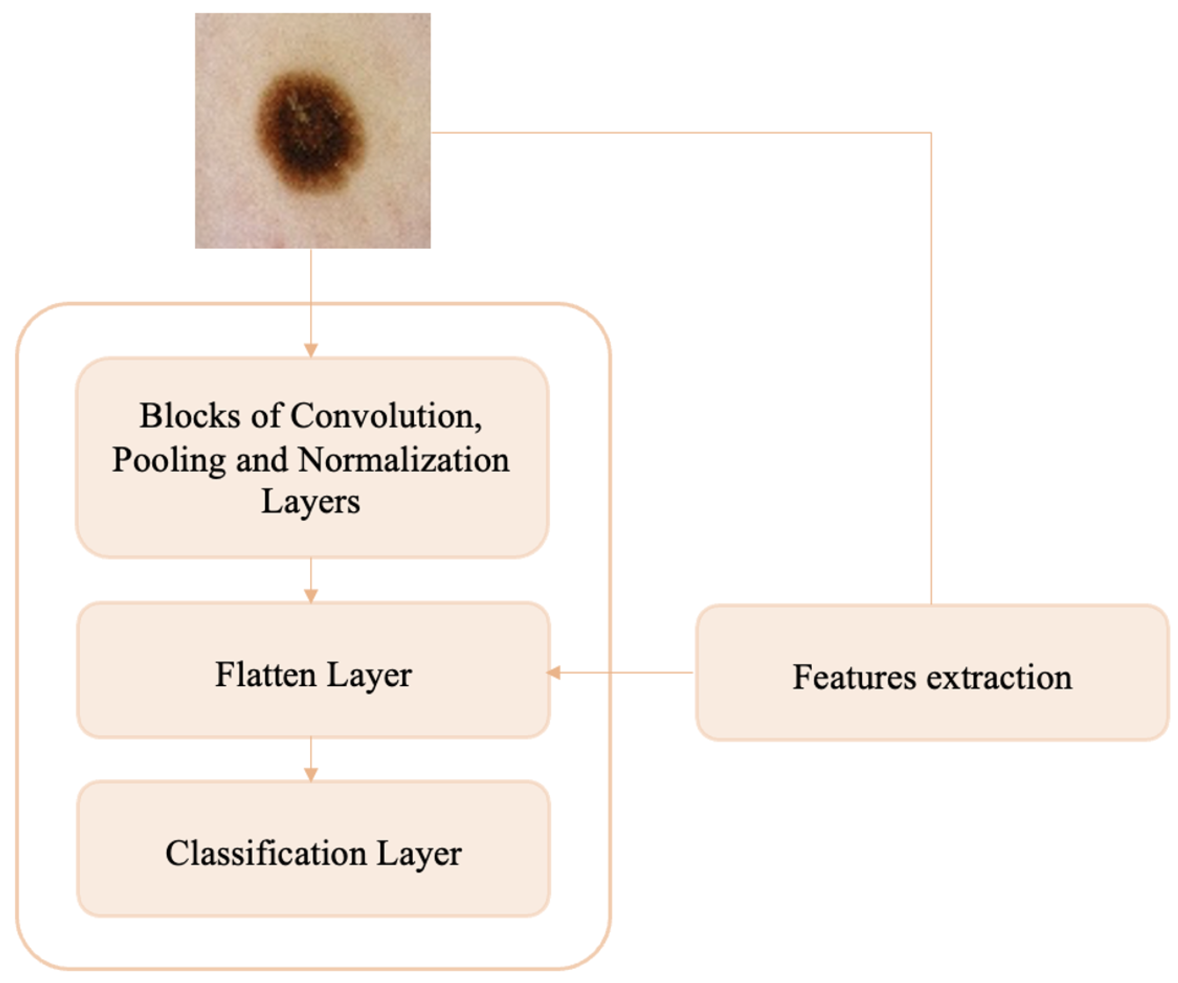The identification of some characteristics, such as symmetry, size, broths, and the presence and distribution of color features (but also blue–white areas, atypical pigmented networks, and globules) is essential for the diagnosis of skin lesions [7]; however, it is a complex and time-consuming procedure that shows a strong dependence on the subjectivity and experience of the physician. These problems necessitate the development of computer-aided diagnostic systems (CAD systems), which generally involve several steps for the analysis and classification of dermoscopic images of skin lesions [8]: preprocessing, segmentation, feature extraction, and classification using ML and DL approaches. Preprocessing aims to attenuate artifacts in the images, which are mainly due to the presence of hairs and marker marks on the lesions, while the segmentation phase aims to isolate the lesion from the surrounding skin and thus extract clinically relevant features. Several solutions have been proposed for these two phases by researchers [9,10,11,12,13,14], many of which are laborious and require the training of additional machine and deep learning models. The feature extraction step can be manual [15] or can be automated using machine learning algorithms. Manual feature extraction in the case of skin lesion classification is based on the methodologies devised by dermatologists for skin cancer diagnosis and, in particular, the ABCDE rule of dermatology. Using machine learning methods, learned features are derived automatically from the datasets and require no prior knowledge of the problem. A variety of approaches are also possible for the final stage of classification: from classical machine learning approaches to state-of-the-art methodologies based on deep convolutional neural networks.

Melanoma detection can be understood as an anomaly detection problem in skin lesions because melanomas represent anomalies (shape, size, color, etc.) in the nevi population. In this paper, we propose an anomaly detection method that involves only the manual and automatic feature extraction and classification steps. Specifically, we develop a custom CNN that, in addition to the dataset of melanoma and nevi images, is trained on additional handcrafted texture features extracted from whole of dermoscopic images. This avoids the segmentation step and could capture some aspects of pathology related to the tissue surrounding the lesions. In addition, no preprocessing is performed on skin lesion images, which reduces the working time. The main contributions of this paper are:

1.

A custom convolutional neural network model with added handcrafted features is proposed that classifies melanomas and nevi accurately without the need for image preprocessing and segmentation.

2.

On the same test dataset, the performance of the proposed model exceeds that of the most widely used pre-trained models for skin lesion classification (ResNet50, VGG16, DenseNet121, DenseNet169, DenseNet201, and MobileNet).

3.

The execution time required by the proposed model to execute the output results is much less than that required by the pre-trained models tested.

4.

The proposed model achieves better accuracy on the ISIC 2016 dataset than other existing deep learning models.

5.

A brief interpretability analysis of the proposed model is performed.

The paper is organized into the following sections. Related work in the areas of skin lesion classification and anomaly detection is reported in Section 2. Section 3 discusses the main challenges and opportunities of skin cancer detection. Section 4 presents the materials used for the present work, namely public datasets of dermoscopic images. Section 5 shows the workflow of the proposed methodology, including the extraction of handcrafted features from dermoscopic images and the construction and training of the CNN network for the melanoma–nevi discrimination task. Section 6 provides details on the settings of the experiments and the creation of the datasets used in training and testing the model. In addition, some ablation experiments and the results obtained for classification are presented. In Section 7, the results obtained by comparing our model with some transfer learning (TL) approaches commonly used in the field of dermatology and with the literature on the ISIC 2016 dataset and DermIS database are discussed. In addition, a brief interpretability analysis of the proposed model is made. In Section 8, the conclusions reached are summarized, and some future arrangements are discussed.

2. Related Works

In the last decade, there has been much increased interest among researchers in developing ML and DL solutions for the classification of skin lesions [16]. This is a nontrivial task that from time to time brings up critical issues that to this day are still unresolved. The basic idea is to be able to provide an accurate diagnostic support tool that is introduced into clinical practice. To date, there are many comparative studies demonstrating that such systems show comparable or even better accuracy than dermatologists [17], and one of these (Moleanalyzer Pro) has been approved for the European market as a medical device [18]. In general, automatic AI-based approaches applied to skin cancer diagnosis can be grouped into two macro-areas [19], one of which involves manual extraction of skin lesion features and subsequent classification by ML algorithms, while the other involves automatic extraction of lesion features and their classification by DL approaches.

2.1. Skin Lesion Classification with Machine Learning Methods

Regarding traditional ML methods, the most widely used classification approach is the Support Vector Machine (SVM). In [10], an automatic method was proposed for multiclass classification of melanoma, dysplastic nevus, and basal cell carcinoma. The work pipeline includes feature extraction of skin lesions (related to shape, edge irregularity, color, and texture), selection of relevant features with a recursive method (RFE), and classification by SVM with a radial kernel (RBF). In [20], lesion segmentation is performed in the gray space, and texture and color features are extracted in the RGB color space. Only the most significant features are selected from the extracted features, which are then classified by a linear SVM model for the melanoma/non-melanoma task. In [21], the authors propose an original and innovative system for automatic melanoma detection (ASMD) that includes: image preprocessing, two-dimensional empirical mode decomposition (BEMD), texture enhancement, manual extraction of entropy and energy features, and binary classification (benign vs. malignant lesion). This last step is operated using an SVM model with an RBF function. All these approaches rely heavily on the preprocessing and segmentation steps of dermatologic images, but they also rely on feature extraction; these are interchanged and combined to find the best classification result. ML algorithms are standard and are already implemented, so not much work can be done on this.

2.2. Skin Lesion Classification with Deep Learning Methods

Regarding DL approaches, the use of pre-trained networks is going mainstream for skin lesion classification. The authors of [22] use transfer learning on InceptionV3, ResNet50, and Denset201 to perform multiclass classification of skin lesions. They remove the output layer from these architectures and add pooling and fully connected layers. In [23], new adversarial example images are created using the fast gradient sign method (FGSM), and some pre-trained networks (VGG16, VGG19, DenseNet101, and ResNet101) are trained and tested with them. Adversarial training allows maximizing the loss for the input image. In some papers, different architectures are used in several different situations. In [24], three pre-trained networks (EfficientNet, SENet, and ResNet) are evaluated in different training scenarios: for the first, segmented images are used; for the second, pre-trained images are used; and for the third the first two solutions are combined. In [25], a pre-trained ResNet52 network is used for skin lesion classification in different training situations: without data augmentation (DA); with DA only for the positive class; with DA for the positive class and downsampling (DS) of the negative class; and with DA only for the positive class but adding other images taken from different datasets. The best solution is one in which data are augmented only on lesions belonging to the positive class. The use of custom CNNs is minor but has still been taken into account [26,27,28].

There is also a hybrid approach that involves both automatic feature extraction using CNNs and manual feature extraction to obtain vectors for inclusion in the network upstream of its decision-making process [29,30]. This approach is still little used in general and even more so in the field of dermatology, but it allows for providing additional important information to the network in order to improve its classification accuracy.

As previously introduced, melanoma detection can be understood as an anomaly detection problem in skin lesions. In anomaly detection, the concept of “abnormality” is contrasted with “normality”, which must be clearly and concretely defined. For the melanoma detection task, normality is represented by the nevi population, while abnormalities are melanomas. This scenario includes several semi-supervised papers in which DL models are trained with only normal data, and anomalies are identified as those data that deviate from the training ones [31,32,33]. In the present work, a supervised anomaly detection approach is proposed in which both normal and anomalous data participate in training the neural network. In addition, the proposed work is in the context of hybrid feature extraction approaches; in fact, important texture features are extracted from dermoscopic images and are injected into the CNN upstream of the classification layer. These features are mixed with those previously extracted from the network, bringing additional information to support correct prediction.

3. Challenges and Opportunities of Skin Cancer Detection

There are several difficulties and challenges in the automatic classification of dermoscopic images by ML and DL methods; these difficulties are still being studied today, and researchers try as much as possible to mitigate them. Some of these are more easily solved than others. For example, real-world clinical validation of the algorithms proposed in the literature is currently lacking [34]. Hence, although many studies show that the performance of DL algorithms equals or even exceeds that of experienced dermatologists in detecting and diagnosing skin lesions [35,36], the performance of these algorithms should also be evaluated on images outside their area of expertise [37] and particularly in a clinical setting (possibly after the clinical diagnosis has been made to avoid bias). In addition, it is unclear how CNNs fare with respect to dermatologists performing visual assessments in the field [38], as all studies comparing man vs. machine performance test dermatologists on their ability to evaluate images and without providing the full picture of metadata normally available in clinical settings. Among the most important and most difficult critical issues to address are those involving the intrinsic characteristics of skin lesions, those related to image quality, and those arising from the way dermatologic datasets are collected.

3.1. Intrinsic Criticalities

Skin lesions have inherent critical issues [39], including: low contrast with the surrounding skin; high variability in shape, size, and location; similarity between healthy and cancerous conditions; and different characteristics according to the patients’ skin conditions. Skin color is a crucial aspect to be addressed [40], although it is still little addressed. In fact, dermoscopic datasets, whether privately collected or publicly available, contain only images of light-skinned people from Europe or East Asia. If trained only on these data, machine learning models cannot provide accurate diagnosis for dark-skinned patients. Therefore, there is a need to expand existing datasets to fill this gap and to avoid incorporating racial disparity, which, unfortunately, exists in dermatology [41], into automatic diagnosis algorithms.

3.2. Image Quality

As previously introduced, other difficulties are related to the quality of the images [42]. Indeed, different acquisition tools and techniques can produce outputs that are very similar from a human perspective but very different for a machine. Poor-quality images are often excluded from studies, but this would lead to unpredictable outputs if the automated model were applied in clinical practice. In addition, the presence of ink marks, rulers, colored discs and hairs tend to deteriorate classification performance. However, including these images in model training could make the model more robust. Model robustness is critical in real-world applications, and it takes on greater importance in medical applications.

3.3. Construction of Datasets

Another important aspect to consider is that for algorithm training, the images used are labeled (diagnosed) by dermatologists; thus, there is a high risk that the networks learn the decision-making process of dermatologists, including all possible biases. Therefore, it would be good to use only biopsy-verified images.

Admitting that we have largely overcome the above challenges, in order to proceed with the acceptance of AI models in dermatological clinical practice, one must be able to understand and explain their decision-making processes. To do so, one must conduct interpretability and explicability analyses of the models in order to interpret and explain their rationale for making a certain decision. This would bridge the distrust—related to not fully understanding—that many physicians place in new and emerging technologies and facilitate their introduction into clinical practice. In addition, it would be good to introduce training courses in the practices of dermatologists since most of them admit that they are not familiar with the subject of AI [43]. The effort produced in addressing the many challenges associated with automated skin cancer detection is certainly repaid by the opportunities that result. In addition to those already mentioned, they include: the ability to avoid unnecessary biopsies or missed melanomas, to make skin diagnoses without the need for physical contact with the patient’s skin, and to reduce the cost of diagnosis and treatment of non-melanoma skin cancer, which turns out to be considerable [44].

4. Materials

The dermoscopic images considered in this paper belong to the International Skin Imaging Collaboration (ISIC) archive [45]. That archive combines several skin lesion datasets and was originally released in 2016 for the challenge called the International Symposium on Biomedical Imaging (ISBI). Specifically, the datasets used for the training phase are the ISBI challenge 2018 and ISBI challenge 2019 datasets, while the dataset that was intended for testing in the ISBI 2018 competition is used for testing. In addition, the ISBI challenge 2016 dataset is used for comparison with the literature. The details of these datasets are given in

Table 1. Summary of the datasets used. The skin lesion classes are: nevi (N)/atypical nevi (AN), malignant melanoma (M), seborrheic keratosis (SK), basal cell carcinoma (BCC), dermatofibroma (DF), actinic keratosis (AK), vascular lesion (VL), and squamous cell carcinoma (SCC).

Dataset	N/AN	M	SK	BCC	DF	AK	VL	SCC	Total
ISIC 2016 [46]	726	173	–	–	–	–	–	–	899
ISIC 2018 [47]	6705	1113	1099	514	115	327	142	–	10,015
ISIC 2019 [48]	12,875	4522	2624	3323	239	867	253	628	25,331

.

For the present study, only N and M image classes are considered to perform the task of discriminating between normal (nevi) and abnormal (melanoma) data. To do so, we simply access the ground truth files in the CSV format provided with the images and select the names of the images for which the diagnosis of melanoma or nevus is expressed with a score of 1 in the associated “MEL” or “NV” boxes, respectively.

5. Methods

The objective of the present work is to try to understand whether by using original (unprocessed) dermoscopic images and additional texture information from whole (unsegmented) images a convolutional neural network can effectively distinguish between nevi and melanomas, which show similar features and are therefore difficult to diagnose. In this section, we present the workflow of the proposed methodology, which is illustrated in Figure 1. Dermoscopic images are given as input to a very simple custom CNN, into the flattened layer of which, during the training phase, previously extracted handcraft features are injected.

5.1. Hadcrafted Feature Extraction

Manual extraction of skin lesion features takes its cue from the ABCDE rule used by dermatologists in clinical practice. The main operations used for the extraction of skin lesion features are: calculation of area, perimeter, major and minor axis length, eccentricity, wavelet invariant moments, and symmetry maps for shape features; calculation of mean, standard deviation, variance, skewness, maximum, minimum, entropy, 1D or 3D color histograms, and autocorrelogram for color features; and calculation of gray-level co-occurrence matrix (GCLM), gray-level length matrix (GLRLM), local binary patterns (LBP), and wavelet and Fourier transforms for texture features. Typically, features extracted from images—after undergoing a selection procedure—constitute the new dataset to be classified. The most commonly used classifiers in dermatology are SVM, K-Nearest Neighbors (KNN), Linear Discriminant Analysis (LDA), and Multilayer Perceptron (MLP) [49,50,51]. The injection of manually extracted features within a neural network, which already extracts features from images, is still a new and untried approach.

In the present work, the handcrafted features considered are only texture features since to extract shape features it is necessary to segment the lesion (an operation deliberately not performed in this work) and, from our practical experience, the color features are already largely captured by the developed CNN. This last statement comes from the results obtained by performing, upstream of neural network training, a color normalization operation on dermoscopic images. The classification performance of melanomas obtained in this situation is poor in general and comparable to that achieved by not performing any preprocessing of the images (see Section 6). In the context of automatic skin lesion diagnosis using ML and DL algorithms, the most widely used texture features are GLCM and LBP; these features are briefly described below.

• GLCM: Gray-level co-occurrence matrices are one of the earliest techniques used for image texture analysis and were proposed by Haralick et al. in 1973 [52]. A co-occurrence matrix, also known as a co-occurrence distribution or gray-level spatial dependence matrix, is a statistical method of image texture analysis that considers the spatial relationship of pixels. It is defined on an image as the distribution of co-occurring values at a given offset and represents the distance and angular spatial relationship over a subregion of the image of specific dimensions. A GLCM is created from a grayscale image and characterizes the texture of an image by calculating the frequency with which pairs of adjacent pixels occur with specific intensity values i and j, and in a specified spatial relationship. The spatial directions, i.e., the directions of analysis, are: horizontal (0°), vertical (90°), and diagonal (−45° and −135°). Given an image I, a random spatial position (h,k), and the offset (${\Delta }_x$,${\Delta }_y$), the co-occurrence matrix is expressed as:

$$G_{i,j}=\sum _{h,k}\left\{\begin{array}{c}1,I(h,k)=i,I(h+{\Delta }_x,k+{\Delta }_y)=j\hfill \\ 0,otherwise\hfill \end{array}\right.$$

(1)

After creating GLCMs, it is possible to derive several statistics from them that provide information about the structure of an image (not the shape, so not the spatial relationships of pixels in an image). These properties [53], shown in Table 2, can be computed over the entire matrix or by considering a window that is moved along the matrix.

Table 2. Properties of GLCM.

Statistic	Equations
Correlation	$$\sum _{i,j}{G}_{i,j}\left[\frac{(i-{\mu }_i)(j-{\mu }_j)}{{\sigma }_i{\sigma }_j}\right]$$ (2)
Homogeneity	$$\sum _{i,j}\frac{G_{i,j}}{1+{(i-j)}^2}$$ (3)
Energy	$$\sqrt{\sum _{i,j}{\left|G_{i,j}\right|}^2}$$ (4)
Contrast	$$\sum _{i,j}{G}_{i,j}{(i,j)}^2$$ (5)
Dissimilarity	$$\sum _{i,j}{G}_{i,j}|i,j|$$ (6)
Entropy	$$\sum _{i,j}{G}_{i,j}(-ln{G}_{i,j})$$ (7)
ASM	$$\sum _{i,j}{G}_{i,j}^2$$ (8)

Table 2. Properties of GLCM.

Statistic	Equations
Correlation	$$\sum _{i,j}{G}_{i,j}\left[\frac{(i-{\mu }_i)(j-{\mu }_j)}{{\sigma }_i{\sigma }_j}\right]$$ (2)
Homogeneity	$$\sum _{i,j}\frac{G_{i,j}}{1+{(i-j)}^2}$$ (3)
Energy	$$\sqrt{\sum _{i,j}{\left|G_{i,j}\right|}^2}$$ (4)
Contrast	$$\sum _{i,j}{G}_{i,j}{(i,j)}^2$$ (5)
Dissimilarity	$$\sum _{i,j}{G}_{i,j}|i,j|$$ (6)
Entropy	$$\sum _{i,j}{G}_{i,j}(-ln{G}_{i,j})$$ (7)
ASM	$$\sum _{i,j}{G}_{i,j}^2$$ (8)

The variables $\mu$ and $\sigma$ are the mean and variance, respectively:

$${\mu }_i=\sum _{i,j}i\left(G_{i,j}\right),{\mu }_j=\sum _{i,j}j\left(G_{i,j}\right)$$

(9)

$${\sigma }_i=\sum _{i,j}{G}_{i,j}{(i-{\mu }_i)}^2,{\sigma }_j=\sum _{i,j}{G}_{i,j}{(j-{\mu }_j)}^2$$

(10)

• LBP: The local binary pattern, a special case of the Texture Spectrum model and first described in 1994, is a simple but very efficient texture operator that labels pixels in an image based on comparison with neighboring pixels [54]. In its simplest form, the LBP feature vector is created by performing the following steps:
  • Division of the image into cells of fixed size.
  • Comparison of the center pixel of each cell with each of its neighbors (top left, top center, top right, right, bottom right, etc.). If the value of the reference pixel is greater than that of the neighboring pixel, a score of 0 is given. Otherwise, the score is 1.
  • Calculation of the histogram of each cell (and, occasionally, normalization of the histogram).
  • Concatenation of the histograms of each cell.

Because of its discriminative power and computational simplicity, the LBP texture operator has become a popular approach in various applications. Perhaps its most important property is its robustness to monotonic changes in grayscale caused, for example, by variations in illumination [55]. A useful extension of the original operator is the so-called uniform pattern; this extension is motivated by the fact that some binary patterns occur in texture images more commonly than others. A local binary pattern is called uniform if the binary pattern contains at most two 0–1 or 1–0 transitions [56]. The uniform model allows for reducing the length of the feature vector and implementing a simple rotation-invariant descriptor.

As previously introduced, in the context of computer-assisted skin lesion diagnosis, the most commonly used texture features are GLCM and LBP. Therefore, in the present work, these features are extracted from dermoscopic images. For the GLCM, to obtain the statistics of contrast, dissimilarity, homogeneity, second angular momentum (ASM), correlation, and energy, Python’s Skimage library was used by setting the offset between pixel pairs to a unity value, choosing four different orientations at 0°, 45°, 90°, and 135°, and making sure that the output was non-symmetrical (the order of the pixel pairs is not ignored) and not normalized by the total number of occurrences accumulated. Doing so yields a total of 24 global textual features for each image. For the LBP, the same Skimage library allows the use of a uniform method with a cell size of 3 × 3, resulting in a total of 26 global textual features for each image.

5.2. Custom CNN with Handcrafted Features

Artificial neural networks (ANNs), inspired by brain connections, are designed to solve complex real-world problems. ANNs have simple architectures organized in layers, each of which is composed of functional units called neurons (or nodes), which are connected by arcs that simulate synaptic connections [57]. Each layer extracts meaningful representations for the problem at hand from the data and processes them before sending them to the next layer. The learning process of a neural network is iterative and relies on adjusting the weights associated with the connections between neurons; changing the weights is based on experience gained in previous iterations.

Convolutional neural networks (CNNs or ConvNets) are artificial neural networks that specialize in computer vision and are inspired by the biological neural networks of the visual cortex [58]. Their structure involves an input, i.e., an image, a feature learning block in which the various hidden layers are responsible for feature extraction, and finally, the output. Each layer consists of elementary computational units that communicate through weighted connections. CNNs are suitable for the field of computer vision precisely because, unlike ANN, they have the units organized in three dimensions (width, height, and depth) and also are connected to only a portion of the previous layer. Layers in CNNs may or may not have trainable parameters; in the latter case, they simply implement functions. The most frequently used types of layers in CNNs are [59]:

• Convolutional layers: Convolutional layers are able to learn local patterns invariant to translation, so that any pattern learned within the image can be recognized even if it is in a different spatial location, and the learning extends to spatial hierarchies of patterns: i.e., the layers learn larger and larger patterns starting from the features of previous layers. This allows the convnet to efficiently learn increasingly complex visual concepts. Convolutional layers contain a series of filters that during the forward phase are run on the input by performing the convolutional (or rather, cross-correlation) operation—that is, the scalar product between the two matrices—from time to time. The result is an m-dimensional feature map, with m equal to the number of filters applied to each layer. The output of the convolution is processed using nonlinear activation functions, such as Hyperbolic, Softmax, Rectified Linear Unit (ReLU), Exponential Linear Unit (ELU), and Scaled Exponential Linear Unit (SELU).
• Pooling layers: Pooling layers aim to sub-sample feature maps by keeping the main information contained in them in order to reduce the number of model parameters and the computational cost. To do this, convolution is again performed between the input image to the layer and a new filter, but in this case, the overlap between the matrices is avoided. The most commonly used pooling filters use mean pooling, the result of which is a matrix in which each value is the average of the submatrices of the source image, and max pooling, the result of which is a matrix in which each value is the maximum value of the submatrices of the source image. The hyperparameters of the pooling layers are the filter size and pitch.
• Normalization layers: Normalization layers are layers for normalizing input data by means of a specific function that does not provide any trainable parameters and only acts in forward propagation. Their contribution is also to reduce the problem of overfitting.
• Fully connected layers: Fully connected layers are layers in which all neurons are connected to all neurons in the previous layer; that is, they use the global connectivity property. The output of such layers is a 1 × 1 × k vector—where k is the number of neurons hosted—containing the activations computed for each neuron. Generally, multiple fully connected layers are used in sequence, the last of which has the parameter k equal to the number of classes in the dataset.

Training DL models with randomly initialized parameters requires a lot of labeled data. In the absence of data, transfer learning is a viable solution because it allows reusing knowledge (the weights) from pre-trained networks on large datasets, such as ImageNet, and achieves good results. The most widely used pre-trained CNN architectures are GoogLeNet, InceptionV3, ResNet, SqueezeNet, DarkNet, DenseNet, Xception, Inception–ResNet, Nasnet, and EfficientNet. In the field of dermatology, although several large public datasets are available, many authors choose to use TL on individual networks [60,61] or by constructing ensemble models from these [62,63,64]. A minority choose to develop custom CNNs based on known networks [65,66,67] or totally new ones [68,69]. In the present work, the custom CNN shown in Figure 2 is developed.

The proposed architecture consists of five convolutional layers followed by five levels of maxpooling and batch normalization. After the last normalization layer, two-dimensional features are flattened into one-dimensional arrays and are given to the output layer consisting of one neuron per class. The number of filters in the first two levels of convolution is 32, in the third and fourth is 64, and in the last level is 128. All convolutional kernels are 3 × 3 in size. Each convolutional layer is followed by a maxpooling layer with a size of 2 × 2 and a batch normalization layer to standardize the inputs. A Leaky Rectified Linear Unit (LeakyReLU) activation function is used in this architecture to introduce nonlinearity into the network. After the last convolutional block, features are flattened by switching from two-dimensional to one-dimensional; thus, features are automatically extracted from the network. To these, handcrafted features acquired using LBP are concatenated, leading to better accuracy than the single-input convolution neural network model (results are discussed in Section 6). In the process of training the proposed architecture, skin lesions are scaled to 224 × 224 pixels and are given as input to the CNN. To reduce computational time, no pre-processing was performed.

6. Results

• Implementation details: A macOs computer with an Apple M1 Pro processor and 16 GB RAM was used for training and validation of the proposed model. Models were created with Spyder 5.1.5 and Python 3.9.12 using the Keras library. Scikit-learn, OpenCV, Pandas, and Numpy were used as dependencies, and Tensorflow, which specializes in effective training of deep neural networks by exploiting graphics cards, served as the backend engine. The choice of the Python language was related to its power and accessibility, which have made it the most popular programming language for data science.
• Details of datasets used: The model was trained with the ISIC 2018 and ISIC 2019 training datasets and was tested on the ISIC 2016 test dataset to ensure comparison of the results obtained with those reported in other papers. As mentioned above, only melanoma and nevi images were selected from each dataset. In the training datasets, the division between classes shows a strong imbalance in favor of the nevi class, whose images are numerically more than three times as numerous as those of melanomas (a widespread phenomenon in the medical field because it is relatively easy to get normal data, but it is quite difficult to get abnormal data). To arrive at a balance between the two classes under consideration, random downsampling (DS) of the nevi class was performed; specifically, the same number of nevi images were selected from the two training datasets such that their sum was equal to the number of melanoma images. The nevi images were randomly selected from each dataset. The initial and final numbers of melanomas and nevi in the two training datasets are reported in Table 3.

Table 3. Number of N and M samples in training datasets.

Dataset	Before			After
	N	M	Tot	N	M	Tot
ISIC 2018	6705	1113	7818	2818	1113	3931
ISIC 2019	12,875	4522	17,397	2818	4522	7340

Table 3. Number of N and M samples in training datasets.

Dataset	Before			After
	N	M	Tot	N	M	Tot
ISIC 2018	6705	1113	7818	2818	1113	3931
ISIC 2019	12,875	4522	17,397	2818	4522	7340

The 10% training data are used as a validation set to provide the impartial process of model training.

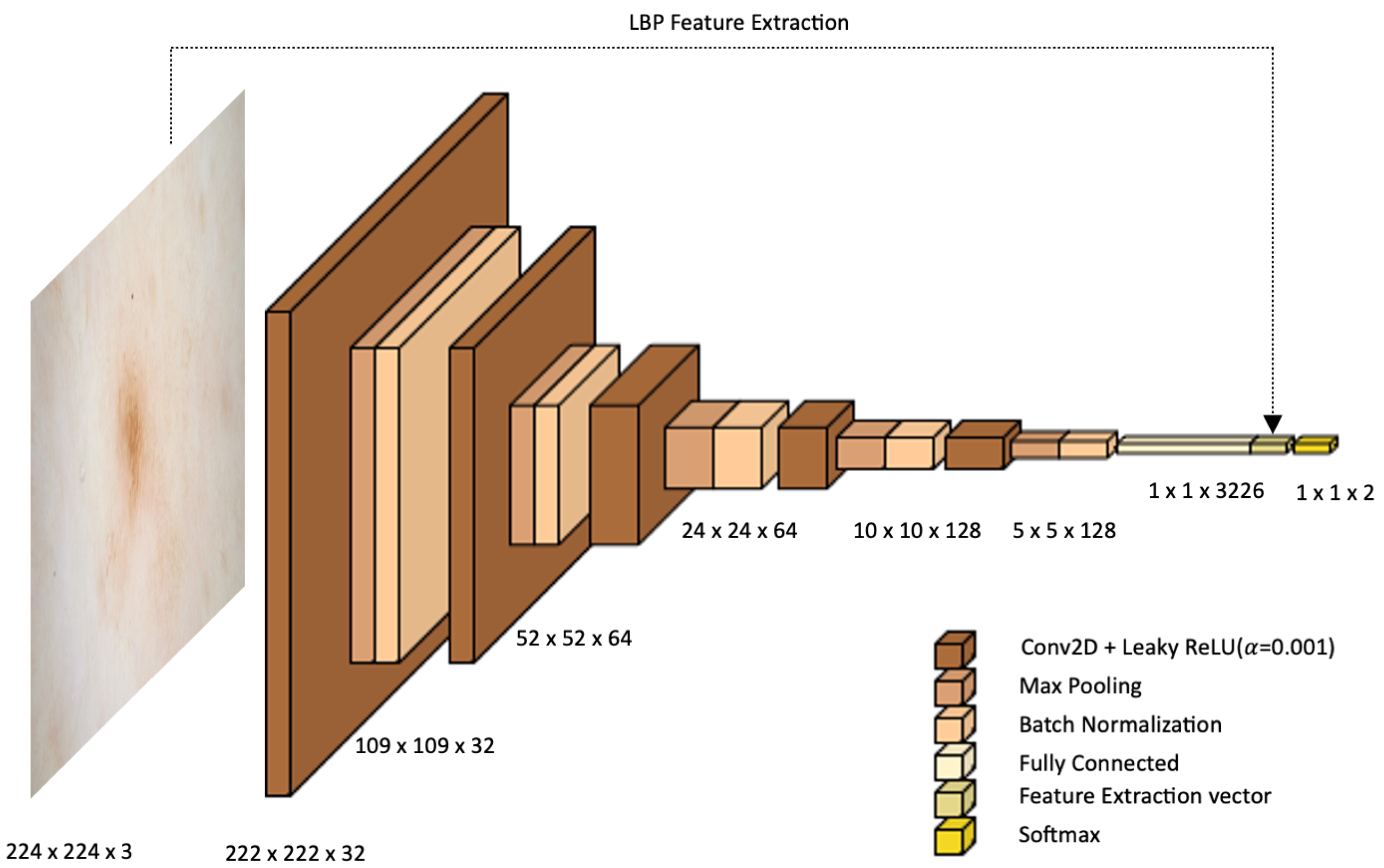
• Network configuration. After testing several configurations obtained by varying the optimizer between Adam, Adamax, and SGD; the initial learning rate between ${10}^{-1}$ and ${10}^{-4}$; and the batch size between 32 and 512; the parameters set for the proposed CNN network were:
  • Optimizer: Adam
  • Initial learning rate: ${10}^{-3}$
  • Loss function: binary cross entropy
  • Number of epochs: 100
  • Batch size: 128
• Classification results: As already anticipated, for the present work, GLCM and LBP texture features were considered for injection into the CNN network to improve its classification performance. Several experiments were conducted to try to find out whether it is convenient to use additional information to that already automatically extracted from the network and, if so, whether it is better to use the two separately or combined. In addition, to understand whether it is necessary to use a complex approach such as a CNN instead of simpler methods, texture features were classified by the most widely used ML methods for skin lesion classification, namely SVM, KNN, and LDA.

  -

  SVM: Both the linear kernel (with the values of the inverse regularization parameter C varied between 1, 10, 100, and 1000) and the RBF and polynomial kernels (with all possible combinations between the values of C equal to the previous ones and the values of the gamma parameter equal to 0.001 and 0.0001) were tested. For both GLCM and LBP feature classification, the best results were obtained using the SVM with the RBF kernel and setting the parameters C = 1000 and gamma = 0.001; for GLCM + LBP feature classification, the best result is obtained with a linear SVM and setting the parameter C = 100.

  -

  KNN: The number of neighbors was varied between 3 and 10. For both GLCM and LBP feature classification, the best result is obtained with K = 9; while for GLCM + LBP combination, the best result is obtained with K = 10.

  -

  LDA: Singular Value Decomposition (SVD) and Least Squares Solution (LSQR) resolution methods were tested, the former of which yielded the best classification performance for all features.

For all ML methods, “best result” means the one that shows the best trade-off between high sensitivity and specificity. The results obtained on the test dataset in the different situations are shown in

Table 4. Comparison of different situations for the classification of melanoma vs. nevus: ML methods for the classification of GLCM features; ML methods for the classification of LBP features; ML methods for the classification of both GLCM and LBP features (G&L); CNN without the injection of handcrafted features (CNN w.f.); CNN with the injection of both GLCM and LBP features (CNN G&L); CNN with the injection of only GLCM features (CNN GLCM); and CNN with the injection of only LBP features (CNN LBP). All values are in percentages.

Method	Accuracy	Sensitivity	Specificity	AUC
SVM GLCM	64.54	76.02	62.38	69.20
KNN GLCM	63.70	64.33	63.59	63.96
LDA GLCM	66.39	63.74	66.89	65.31
SVM LBP	74.26	69.59	75.14	72.36
KNN LBP	70.83	70.76	70.85	70.80
LDA LBP	75.83	62.57	78.33	70.45
SVM G&L	78.52	74.27	79.32	76.79
KNN G&L	72.50	74.85	72.06	73.46
LDA G&L	79.44	73.68	80.53	77.11
CNN w. f.	81.11	75.44	82.18	78.81
CNN G&L	81.57	68.42	84.05	76.23
CNN GLCM	80.83	75.44	81.85	78.64
CNN LBP	82.50	76.61	83.61	80.11

.

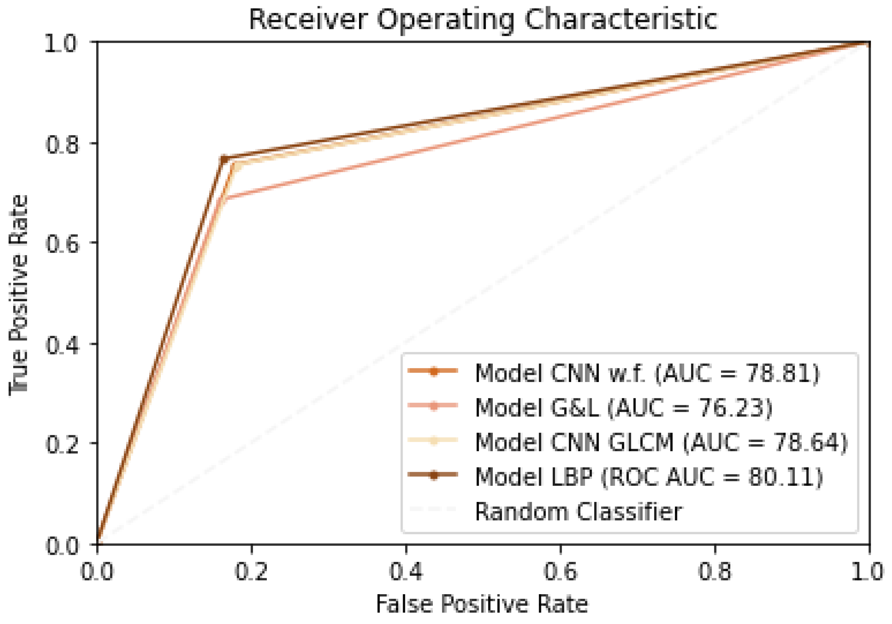
The ML methods show similar sensitivity values to those obtained with the various CNN networks, but they have lower specificity, accuracy, and AUC. Looking at the results obtained with CNNs, it is evident from the results that none of the situations is clearly superior to the others, but the best is the one in which LBP texture features are injected into the proposed CNN network. For these latter four situations, ROC curve plots are shown in Figure 3.

One might also ask whether the LBP features extracted from the images are all relevant or whether a selection of the most significant ones should be performed. In this regard, two alternative scenarios were simulated in which Principal Component Analysis (PCA) was applied to reduce the dimensionality of the features to 1/3 and 1/2 of their original sizes. The results obtained by training the proposed CNN with the addition of these reduced features are shown in

Table 5. Comparison of classification results obtained by training the CNN network with all the LBP features and with a portion of them (PCA(1/3) and PCA(1/2)). All values are in percentages.

Method	Accuracy	Sensitivity	Specificity	AUC
PCA(1/3)	82.41	60.82	86.47	73.64
PCA(1/2)	82.31	71.35	84.38	77.86
CNN LBP	82.50	76.61	83.61	80.11

along with those obtained by considering all the original features.

In the PCA(1/3) case, sensitivity increases compared with the situation where feature dimensionality is not reduced, but specificity decreases greatly. In contrast, in the PCA(1/2) case, the results are lower than the CNN LBP situation for all metrics. From the results obtained, it can be inferred that it is not necessary to perform dimensionality reduction of LBP texture features since they are all important for classification of skin lesions.

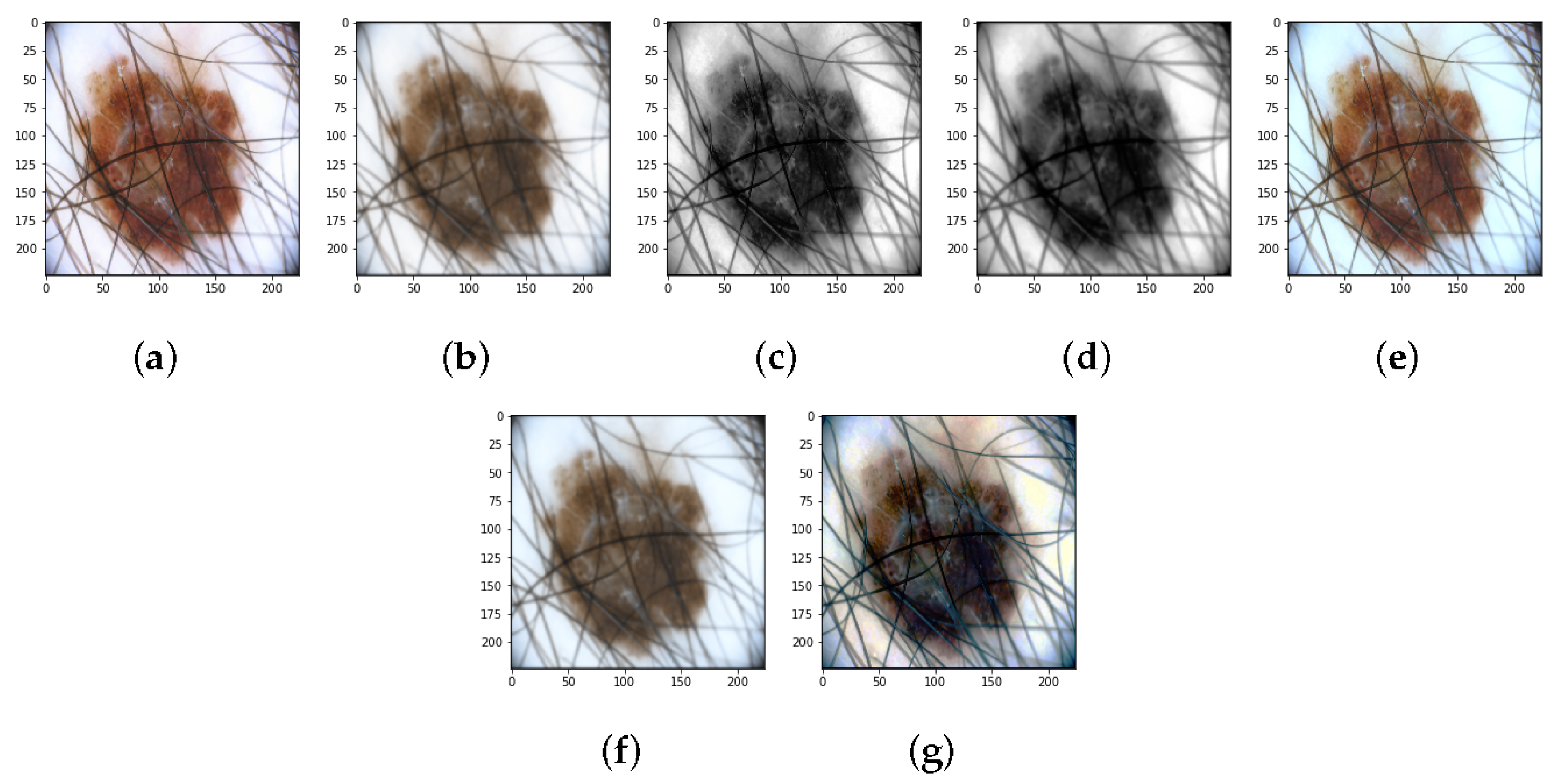
In addition, the present work aims to investigate whether a preliminary image preprocessing step is necessary for the addressed anomaly detection task. In this regard, a comparison is made between the performance obtained by training the custom CNN LBP with the original images and with images preprocessed using the main techniques used in the field of dermatology, as is discussed briefly below.

• Gaussian filter (GF) is a linear smoothing filter that operates as a kind of low-pass filter [70]. It is a widely used preprocessing method in image processing and computer vision to attenuate noise. In the present work, the standard deviation for the Gaussian kernel ($\sigma$) is set to 1, 3, and 5; the smoothing operation is performed identically in all directions, resulting in a filtering action independent of the orientation of the structures in the image.
• Histogram Equalization (HE) is the most widely used global method for calibrating contrast in images and is based on the idea of reassigning pixel intensity values to make the intensity distribution maximally uniform [71].
• Color Normalization (CN) is a technique widely used in computer vision to compensate for illumination variations in images. The method chosen for the present work is based on the technique of color constancy [72] that ensures that the perceived color of the image remains the same under different illumination conditions in order to facilitate the classification algorithm.

Various combinations of the techniques just described were also tested: GF + HE, GF + CN, and HE + CN. In such combinations, the Gaussian filter was set with $\sigma =1$, which has been shown to yield the best classification results. The results of applying the various preprocessing methods to a skin lesion image are shown in Figure 4.

A comparison of the classification results obtained by training the neural network with original and preprocessed images is shown in

Table 6. Comparison of classification results obtained by training the CNN network with preprocessed and original images (CNN LBP is the CNN trained with original images, i.e., images without preprocessing). All values are in percentages.

Method	Accuracy	Sensitivity	Specificity	AUC
CNN GF ($\sigma =1$)	80.09	71.35	81.74	76.54
CNN GF ($\sigma =3$)	84.07	0	99.89	49.95
CNN GF ($\sigma =5$)	83.43	40.35	91.53	65.94
CNN HE	77.59	77.78	77.56	77.68
CNN CN	83.98	67.25	87.13	77.19
CNN GF + HE	83.89	63.74	87.68	75.71
CNN GF + CN	75.93	81.87	74.81	78.34
CNN HE + CN	83.61	63.13	87.46	75.31
CNN LBP	82.50	76.61	83.61	80.11

.

It can be seen from the results that: (1) the Gaussian filter with $\sigma =3$ and $\sigma =5$ leads to high specificity values but very low sensitivity; (2) color normalization (CNN CN), Gaussian filtering combined with histogram equalization (CNN GF + HE), and the combination of histogram equalization and color normalization (CNN HE + CN) allows for the obtainment of higher specificity values—and therefore higher accuracy—than that obtained without preprocessing; however, in all these situations, the sensitivity, which reflects the accuracy in correctly classifying melanomas and is therefore a parameter of utmost importance for the specific application (anomaly detection in the medical field), is much lower than that obtained with CNN w. p.; (3) application of the Gaussian filter with $\sigma =1$ leads to classification results similar to those obtained by training the network with the original images, but lower; (4) the best trade-off between sensitivity, specificity and accuracy seems to be achieved by the CNN network trained using the original images.

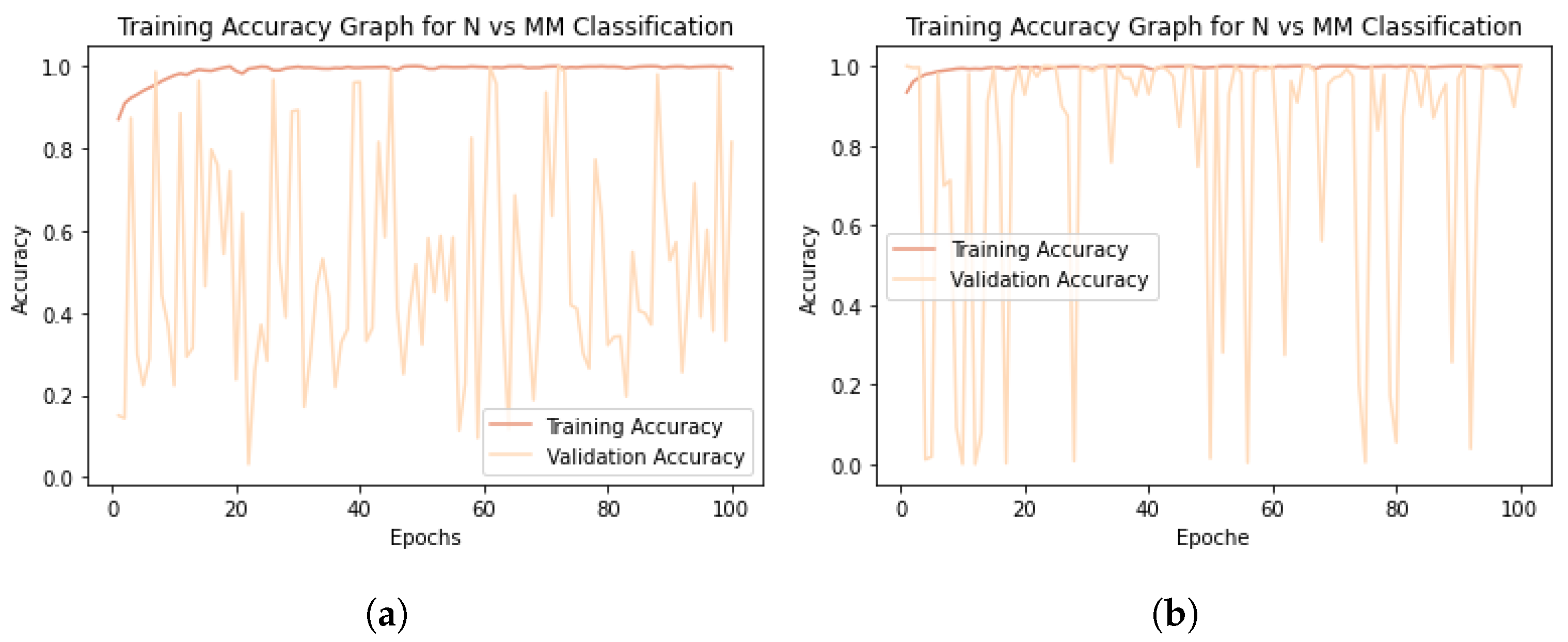
Once the best solution for melanoma detection was identified—which was obtained by adding the texture information captured by the LBP operator from the unprocessed images to the CNN network—we wanted to check whether the selection of the training dataset made to balance the two classes was the best one. In this regard, the proposed balancing situation—the results of which have already been shown in Table 4—is compared with the following two: (1) the imbalance between the classes is not balanced, and therefore, the training set includes all nevi and melanoma images (scenario named M/Ntot). In this case, the number of nevi is more than three times the number of melanomas; (2) to make the number of melanomas approach the total number of nevi, data augmentation is applied on the melanoma images until the number of melanomas is tripled (scenario named DA Mx3). The operations performed to increase the number of images in the training dataset are: rotation (range = 20), width shift (range = 0.1), height shift (range = 0.1), shear (range = 0.3), zoom (range = 0.3), horizontal flip, and fill mode = ’nearest’. The results obtained by training the network with these new datasets and the comparison without using DA are shown in

Table 7. Comparison of results obtained using different distributions of M and N in the training dataset. Performance results are in percentages.

Method	M	N	Accuracy	Sensitivity	Specificity	AUC
M/Ntot	5635	19,580	45.00	73.68	39.60	56.64
DA Mx3	16,905	19,580	84.17	0.00	100.00	50.00
CNN LBP	5635	5636	82.50	76.61	83.61	80.11

.

Paradoxically, by not balancing the classes and thus having one-third as many melanomas as nevi, the specificity is much higher than the sensitivity; on the other hand, as the number of melanomas increases, the ability of the network to recognize nevi also increases, but the network has zero sensitivity, indicating that no melanomas were classified correctly. The results obtained, although it may not seem like it, are “lucky” results; in fact, they could have been even worse considering the fact that during training, the performance of the models on the validation dataset was anything but consistent in both scenarios previously described. Figure 5 plots the accuracy curves obtained during training in the M/Ntot Figure 5a and DA Mx3 Figure 5b situations.

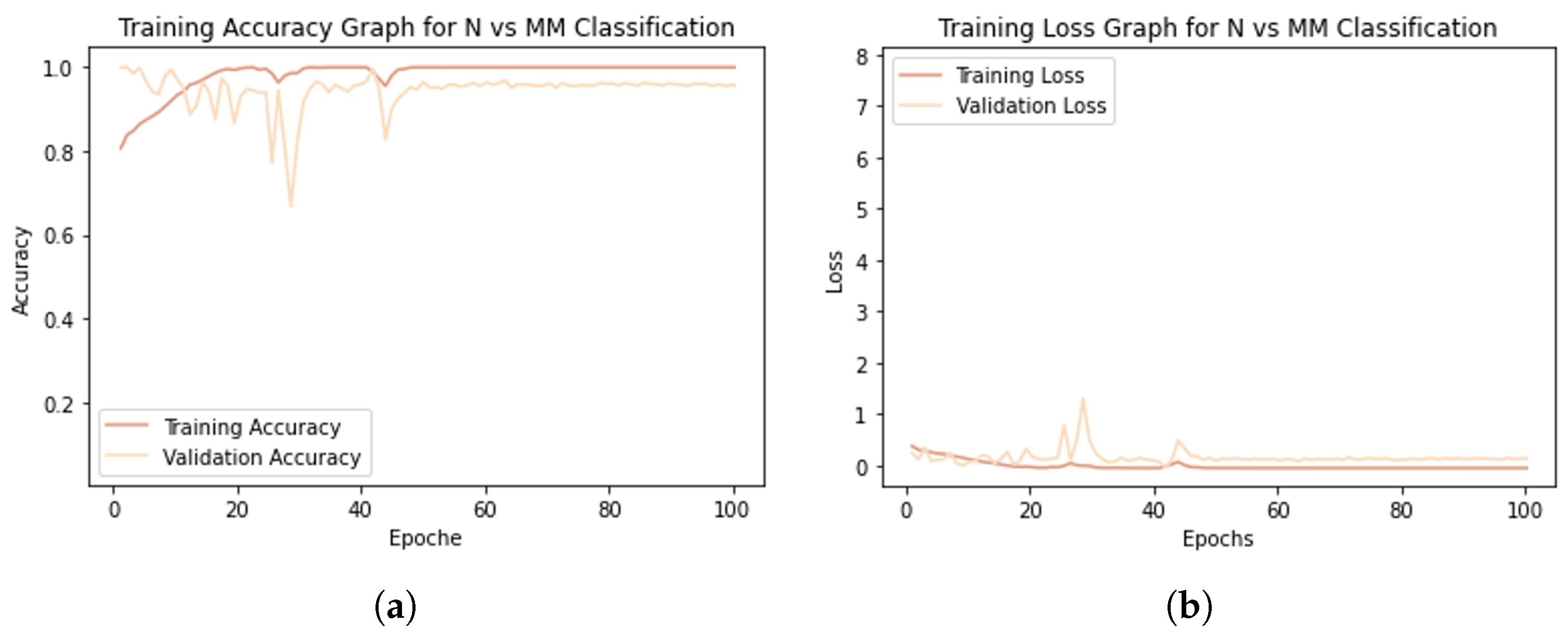
Having verified that the best classification results for melanoma detection are obtained by adding the texture information captured using the LBP operator to the CNN network and dividing the two classes equally without applying DA techniques, we refer to this situation below by talking about the “proposed work”. Then, the accuracy and loss plots of the training and validation sets related to the proposed work are shown in Figure 6.

The model shows an excellent learning rate, as the training accuracy increases with the number of epochs (Figure 6a), and the validation accuracy, although it tends to decrease at first, stabilizes not far from the training curve. Both training loss and validation loss decrease to the point of stability (Figure 6b). Training reaches convergence after about 50 epochs. The small gap between the training and validation curves shows that the model is not affected by overfitting.

The results shown by the validation curves are very different from those obtained on the test set (see Table 7). This could stand to mean that: (1) because the ISIC 2019 dataset is more numerous than the ISIC 2018 dataset, the network learned more about the characteristics of this dataset, and that (2) the 10% of the training dataset intended to constitute the validation set (obtained by means of the validation split function in Keras) contains many more ISIC 2019 images than ISIC 2018 images, thus making the results obtained on the validation and test sets not coincide. However, good generalization capabilities across similar datasets would be expected from a model showing these curves; in fact, although they were collected in different years and intended for different challenges, the ISIC 2018 and ISIC 2019 datasets both contain dermoscopic images. It is beyond the scope of this paper to investigate possible differences in the acquisition or preprocessing of the images that make up the two datasets, which might be a good reason to balance the training dataset not only from the point of view of classes (as many melanomas as nevi) but also from the point of view of the source from which the images come (as many ISIC 2018 images as ISIC 2019 images).

Section 7 reports and discusses the results obtained from comparing the proposed model with the most widely used pre-trained models for skin lesion classification: VGG16, ResNet50, MobileNet, DenseNet121, DenseNet169, and DenseNet201. In addition, the performances of the proposed network on the ISIC 2016 dataset and on the DermIS database are compared with other state-of-the-art methods from the literature.

7. Discussion

The purpose of the proposed work is an in-depth study of the analysis and classification of dermoscopic images. In fact, we want to understand whether the hard work of preprocessing images of skin lesions—aimed at the elimination of hairs, marker marks, air bubbles, etc.—is really essential for the classification of melanomas vs. nevi and whether useful information can be drawn not only from the lesions under examination but also from the area of skin surrounding them. In fact, imagining that the region of skin surrounding the lesions has also undergone some change that is, however, not yet visible to the naked eye, not taking it into consideration would miss important and potentially useful information for classification/diagnosis purposes. Thus, the proposed method is aimed at examining these aspects and involves training a custom CNN with images that have not undergone any kind of preprocessing to improve their appearance and adding texture information related to whole images (lesion + surrounding skin). This method is compared with the most widely used pre-trained networks in the field of dermatology and other state-of-the-art methods using ISIC 2016 as a test set.

7.1. Comparison with Common Pre-Trained Networks

Although public dermatology datasets are large enough to successfully train even complex custom neural networks, the use of pre-trained networks— typically on the ImageNet dataset—is widespread. In the dermatology field, the most widely used are: VGG16, ResNet50, MobileNEt, DenseNet121, DenseNet169, and DenseNet201. A comparison of the proposed model is performed with all these networks to see if it is the best one for the task at hand. The results of the comparison between the proposed network and the tested pre-trained models are shown in

Table 8. Comparison of proposed work for the classification of melanoma vs., nevus with common pre-trained networks. Performance values are in percentages.

Network	Accuracy	Sensitivity	Specificity	Total Parameters	Trainable Parameters	Time per Epoch
VGG16	61.72	80.60	58.56	∼124 M	∼200 k	≃56’
ResNet50	53.63	84.21	48.54	∼3.5 M	∼100 k	≃16’
MobileNet	60.05	86.55	55.64	∼7 M	∼100 k	≃4’
DenseNet121	54.46	90.64	50.78	∼13 M	∼165 k	≃12’
DenseNet169	59.05	88.30	54.18	∼24 M	∼200 k	≃14’
DenseNet201	59.80	86.55	55.35	∼18.5 M	∼200 k	≃19’
Proposed work	82.50	76.61	83.61	∼150 k	∼150 k	≃4’

.

Pre-trained models have millions of pre-trained parameters and only a small fraction of trainable parameters, whereas in a custom CNN, since there is no prior knowledge, all parameters are trainable. Information already learned from pre-trained networks can be very useful in classifying new data, but it is not always the best solution, especially when the pre-trained and newly trained data do not have similar characteristics. From the results, it can be seen that the proposed model, in addition to being better able to distinguish melanomas and nevi than the other networks, takes much less time for each epoch of training because of the simplicity of its architecture. This is no small detail considering that many epochs are planned for the training phase.

7.2. Comparison with the Literature

The different existing works regarding the melanoma vs. nevi classification task and using ISIC 2016 as the test dataset, described in [19], are reported below and are finally compared with the proposed model. In [73], the authors propose three different scenarios for using the VGG16 network. First, they train the network from scratch, obtaining the least accurate results. Then, they apply the TL method, which turns out to be better than the first method but suffers from the phenomenon of overfitting. Finally, they apply fine-tuning, obtaining the best results. The authors of [30] propose a framework that performs image preprocessing and performs the classification task using a hybrid CNN consisting of three feature extraction blocks whose results are merged to provide the final output. In [74], an approach is proposed in which shape, color, and texture features are extracted from previously segmented skin lesion images and then concatenated to features automatically extracted from a custom CNN.

The comparison between the performance achieved by the proposed model and that of works reported in the literature is summarized in

Table 9. Comparison of proposed work for the classification of melanoma vs. nevus with existing work on ISBI 2016 dataset. All values are in percentages. The symbol “-” indicates missing information.

Author and Year	Accuracy	Sensitivity	Precision	Specificity	AUC
Lopez et al. [73] 2017	81.30	78.70	79.70	-	-
Kotra et al. [30] 2021	93.00	-	-	-	-
Hasan et al. [74] 2022	-	92.00	92.00	-	96.00
Proposed work	98.15	97.33	93.59	98.35	97.84

.

On the 2016 ISIC dataset, the performance of the model is very high and reflects the accuracy and loss curves shown in Section 6 (Figure 6). Both in terms of accuracy and in terms of sensitivity, specificity, and AUC score, the proposed model outperforms the models reported in the literature. Whether this result is due to the fact that, in contrast to [30], the images were not preprocessed; or to the fact that, in contrast to [74], the texture features were extracted from the entire image and not only from the segmented lesion; or again, that both may have contributed to the result is not known for sure.

To show the robustness of the proposed work, an external validation was conducted using the online public database Dermatology Information System (DermIS) [75]. This dataset, which contains 1000 dermoscopic images, of which 500 are benign and 500 are malignant, is the largest public dataset after the ISIC archive. Containing a limited number of data, the DermIS dataset is integrated with other public or private datasets, and classification results are reported globally but not for the split datasets, thus preventing comparison with the literature. A paper was identified that reports classification results on the DermIS dataset not combined with other datasets, the comparison of which with the proposed method is shown in

Table 10. Comparison of proposed work for the classification of melanoma vs. nevus with existing work on DermIS database. All values are in percentages. The symbol “-” indicates missing information.

Author and Year	Accuracy	Sensitivity	Precision	Specificity	AUC
Abbes et al. [76] 2017	76.9	97.40	-	48.40	-
Proposed work	81.50	92.71	74.79	71.15	81.93

.

Although the sensitivity of the model proposed in [76] is higher than that obtained in the present work, the specificity is much lower. This leads to a good ability to classify melanomas correctly, but there is a high rate of false positives, which, although less severe than false negatives, lead to increased costs for patients, who will have to undergo unnecessary additional visits and diagnostic tests. The proposed model once again shows good results compared with the literature.

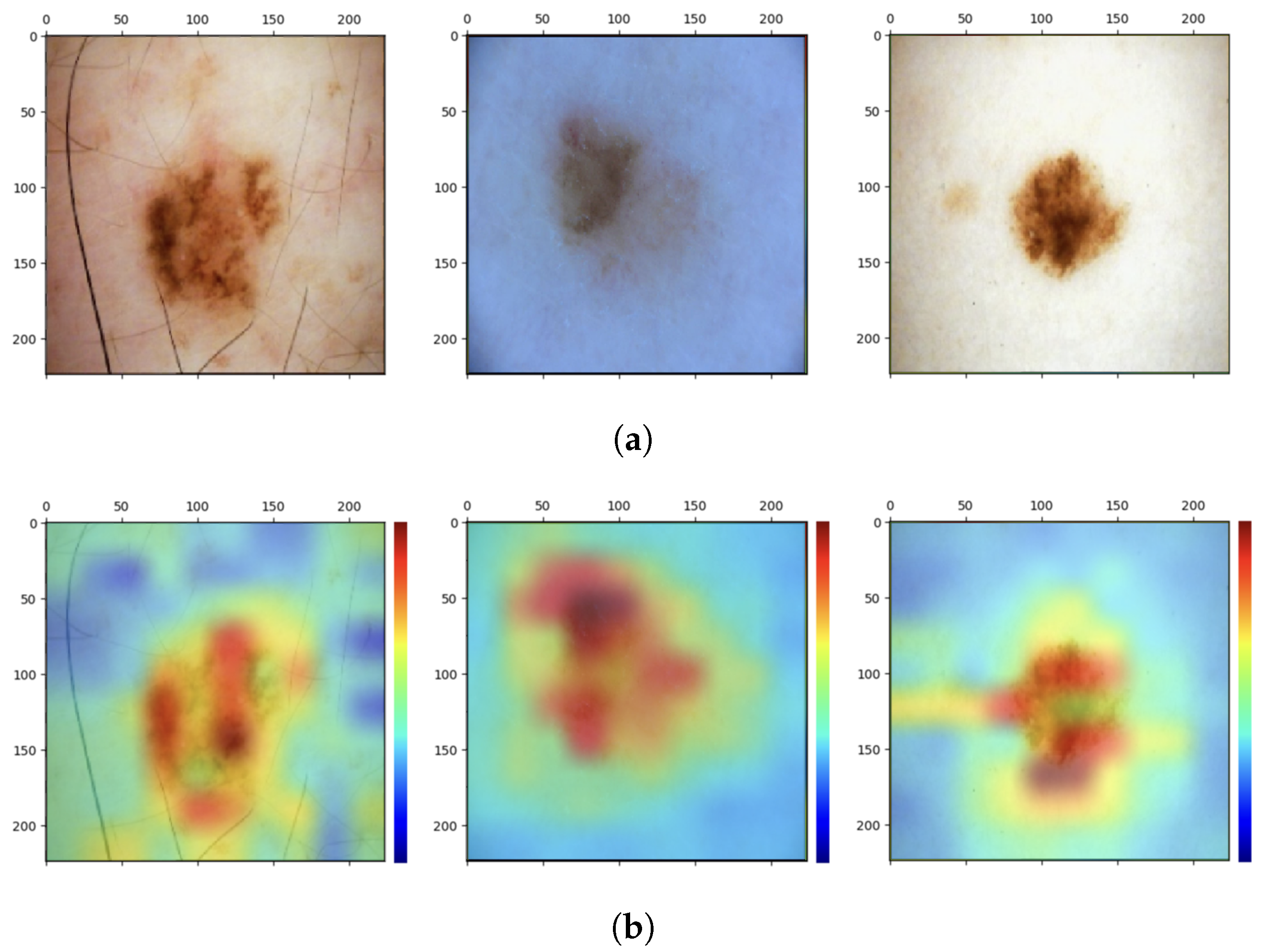
7.3. Analysis of Interpretability and Limitations of the Proposed Model

With the interpretability analysis of neural networks, it is possible to have a visual explanation of the decisions made by the so-called “black-box”. For such analysis, the Grad-CAM algorithm is used in the present work. This algorithm uses the gradient information (global mean) flowing into the last convolutional layer of the CNN to assign importance values (weights) to each neuron for a particular decision of interest [77]. The convolutional layers naturally retain spatial information that is lost in the fully connected layers; therefore, the last convolutional layers can be expected to have the best trade-off between high-level semantics and detailed spatial information. Neurons in these layers search for class-specific semantic information in the image (e.g., parts of objects). The heat map of the image that results from applying this algorithm highlights the features of the image. The Grad-CAM algorithm is applied on the last convolutional layer of the proposed custom CNN, that is, before the injection of texture features. Some results obtained are shown in Figure 7.

As can be seen, the network focuses mainly on the pixels of the skin lesion; from here emerges the contribution of adding texture features extracted not only from the lesion but also from what surrounds it, which is not automatically considered by the neural network and which could be useful for the correct classification of the lesion. However, injecting into the network additional features extracted from images that have not undergone any preprocessing of cropping out parts that are not relevant to the diagnosis may lead the network to attribute to one of the two classes a specific feature that is not related to the pathology at all. These are spurious correlations, and in the present case, these correlations involve dark image contours due to the image acquisition process and associated with the class of melanoma (Figure 8).

Such images are classified correctly, but interpretability analysis shows that to arrive at the correct result, even before feature injection, the network focuses on regions of the image that are not diagnostically important. If the network already sees these details as possible important features for assigning the N or M label to the images, it is possible that the additional feature vector is going to contribute in the same direction by emphasizing the spurious correlation. One would then need to conduct an analysis on the outcome of the classification after appropriately cropping the images so as to eliminate the black edge disturbance while retaining as much of the surrounding tissue as can be saved.

Another important aspect to consider is that the proposed model is among the methodologies that can classify images of single skin lesions but not total body images. The single-lesion approach allows the application of some dermatologic rules, such as the ABCDE rule, but does not allow consideration of the global picture of patients’ skin lesions (as opposed to dermatologic examinations in which macro-screening is performed). In fact, with this approach, it is not possible to assess the presence of the so-called “ugly duckling”: that is, a nevus that is different from a subject’s other nevi and is therefore suspect [78]. The underlying concept is that most normal lesions resemble each other, whereas melanomas differ in size, shape, and color just like they are ugly ducklings (abnormal data in the context of anomaly detection). The total body photography (TBP) technique allows photographs of the entire body or portions of the body (wide-field approaches) to be acquired, allowing lesions to be mapped and the entire skin surface of the patient to be monitored [79]. This technique was combined with DL techniques using 2D [80,81,82] and 3D [83] images and showed excellent classification performance. The advantages of using this technique in computer-assisted diagnosis systems relate to the possibility of getting an overview of patients’ skin lesions, the possibility of implementing teledermatology since there is no specific acquisition instrumentation but images can be taken using traditional cameras, and finally, the possibility of assessing the appearance of new skin lesions during follow-up. There are limitations, however, in that, compared with the single-lesion method, the total-body approach implies reduced image quality (even using high-resolution cameras, the image quality of skin lesions is lower than that obtained with dermoscopy), and in addition, the absence of public databases makes comparison with the literature impossible.

8. Conclusions and Future Work

In the present work, the identification of cutaneous melanoma is intended as an anomaly detection problem for which a simple custom CNN is proposed, in which additional texture information from dermoscopic images of skin lesions is included to aid in its increased classification performance for the melanoma vs. nevi task. The goal, in addition to creating a network that is accurate in melanoma detection (anomaly detection), is to test whether such a network, trained on unprocessed images from which features are extracted in full, can achieve high performance. In fact, although lesion segmentation allows the ABCD rules commonly used by dermatologists for the examination of skin lesions to be applied, it is not necessarily the case that the features of the tissue surrounding the lesions do not contain important information overlooked in clinical diagnosis. Several experiments were conducted to (1) demonstrate that simple ML models are not suitable for the purpose of this work; (2) show how there is no need to operate dimensionality reduction of extracted features, which are found to be totally important; (3) demonstrate that preprocessing of dermoscopic images is not strictly necessary; and (4) in the present case, the data augmentation technique does not improve classification performance but even worsens it. The proposed network, trained on the ISIC 2018 and ISIC 2019 datasets, shows better results than the most commonly used pre-trained networks in dermatology, especially with regard to computational cost. Moreover, on the ISIC 2016 dataset, the proposed model achieves very high performance that is higher than that reported in the literature. On the DermIS database, the proposed model also performs well. This could mean that image preprocessing is not so necessary but also that image segmentation from which additional information is then extracted tends to leave out important aspects of the images not necessarily related to the lesion. An interpretability analysis is then conducted, which shows that additional texture information related to the unsegmented whole images may add to the network classification—which instead dwells on the skin lesion—but also that these features could contribute to increased spurious correlations. Therefore, probably a preliminary step of partial elimination of any disturbances, such as black image contours, could lead to improved classification results. Future work will go in this direction.

References

1. Apalla, Z.; Nashan, D.; Weller, R.B.; Castellsagué, X. Skin Cancer: Epidemiology, Disease Burden, Pathophysiology, Diagnosis, and Therapeutic Approaches. Dermatol. Ther. 2017, 7 (Suppl. S1), 5–19. [Google Scholar] [CrossRef]
2. Hu, W.; Fang, L.; Ni, R.; Zhang, H.; Pan, G. Changing trends in the disease burden of non-melanoma skin cancer globally from 1990 to 2019 and its predicted level in 25 years. BMC Cancer 2022, 22, 836. [Google Scholar] [CrossRef] [PubMed]
3. Hasan, M.R.; Fatemi, M.I.; Khan, M.M.; Kaur, M.; Zaguia, A. Comparative Analysis of Skin Cancer (Benign vs. Malignant) Detection Using Convolutional Neural Networks. J. Healthc. Eng. 2021, 2021, 5895156. [Google Scholar] [CrossRef]
4. Lacy, K.; Alwan, W. Skin cancer. Medicine 2013, 41, 402–405. [Google Scholar] [CrossRef]
5. Lopes, J.; Rodrigues, C.M.P.; Gaspar, M.M.; Reis, C.P. How to Treat Melanoma? The Current Status of Innovative Nanotechnological Strategies and the Role of Minimally Invasive Approaches like PTT and PDT. Pharmaceutics 2022, 14, 1817. [Google Scholar] [CrossRef]
6. Mehta, P.; Shah, B. Review on techniques and steps of computer aided skin cancer diagnosis. Procedia Comput. Sci. 2016, 85, 309–316. [Google Scholar] [CrossRef]
7. Youssef, A.; Bloisi, D.D.; Muscio, M.; Pennisi, A.; Nardi, D.; Facchiano, A. Deep Convolutional Pixel-wise Labeling for Skin Lesion Image Segmentation. In Proceedings of the 2018 IEEE International Symposium on Medical Measurements and Applications (MeMeA), Rome, Italy, 11–13 June 2018; pp. 1–6. [Google Scholar]
8. Masood, A.; Ali Al-Jumaily, A. Computer aided diagnostic support system for skin cancer: A review of techniques and algorithms. Int. J. Biomed. Imaging 2013, 2013, 323268. [Google Scholar] [CrossRef]
9. Zanddizari, H.; Nguyen, N.; Zeinali, B.; Chang, J.M. A new preprocessing approach to improve the performance of CNN-based skin lesion classification. Med. Biol. Eng. Comput. 2021, 59, 1123–1131. [Google Scholar] [CrossRef] [PubMed]
10. Chatterjee, S.; Dey, D.; Munshi, S. Integration of morphological preprocessing and fractal based feature extraction with recursive feature elimination for skin lesion types classification. Comput. Methods Programs Biomed. 2019, 178, 201–218. [Google Scholar] [CrossRef]
11. Schaefer, G.; Rajab, M.I.; Celebi, M.E.; Iyatomi, H. Colour and contrast enhancement for improved skin lesion segmentation. Comput. Med. Imaging Graph. 2011, 35, 99–104. [Google Scholar] [CrossRef] [PubMed]
12. Yuan, Y.; Chao, M.; Lo, Y.C. Automatic skin lesion segmentation using deep fully convolutional networks with jaccard distance. IEEE Trans. Med. Imaging 2017, 36, 1876–1886. [Google Scholar] [CrossRef] [PubMed]
13. Jafari, M.H.; Karimi, N.; Nasr-Esfahani, E.; Samavi, S.; Soroushmehr, S.M.R.; Ward, K.; Najarian, K. Skin lesion segmentation in clinical images using deep learning. In Proceedings of the 2016 23rd International Conference on Pattern Recognition (ICPR), Cancun, Mexico, 4–8 December 2016; IEEE: Piscataway, NJ, USA, 2016; pp. 337–342. [Google Scholar]
14. Xie, F.; Yang, J.; Liu, J.; Jiang, Z.; Zheng, Y.; Wang, Y. Skin lesion segmentation using high-resolution convolutional neural network. Comput. Methods Programs Biomed. 2020, 186, 105241. [Google Scholar] [CrossRef] [PubMed]
15. Barata, C.; Celebi, M.E.; Marques, J.S. A survey of feature extraction in dermoscopy image analysis of skin cancer. IEEE J. Biomed. Health Inform. 2018, 23, 1096–1109. [Google Scholar] [CrossRef]
16. Hasan, M.K.; Ahamad, M.A.; Yap, C.H.; Yang, G. A survey, review, and future trends of skin lesion segmentation and classification. Comput. Biol. Med. 2023, 155, 106624. [Google Scholar] [CrossRef] [PubMed]
17. Dick, V.; Sinz, C.; Mittlböck, M.; Kittler, H.; Tschandl, P. Accuracy of computer-aided diagnosis of melanoma: A meta-analysis. Jama Dermatol. 2019, 155, 1291–1299. [Google Scholar] [CrossRef] [PubMed]
18. Haenssle, H.A.; Fink, C.; Toberer, F.; Winkler, J.; Stolz, W.; Deinlein, T.; Zukervar, P. Man against machine reloaded: Performance of a market-approved convolutional neural network in classifying a broad spectrum of skin lesions in comparison with 96 dermatologists working under less artificial conditions. Ann. Oncol. 2020, 31, 137–143. [Google Scholar] [CrossRef]
19. Grignaffini, F.; Barbuto, F.; Piazzo, L.; Troiano, M.; Simeoni, P.; Mangini, F.; Pellacani, G.; Cantisani, C.; Frezza, F. Machine Learning Approaches for Skin Cancer Classification from Dermoscopic Images: A Systematic Review. Algorithms 2022, 15, 438. [Google Scholar] [CrossRef]
20. Bansal, P.; Vanjani, A.; Mehta, A.; Kavitha, J.C.; Kumar, S. Improving the classification accuracy of melanoma detection by performing feature selection using binary Harris hawks optimization algorithm. Soft Comput. 2022, 26, 8163–8181. [Google Scholar] [CrossRef]
21. Cheong, K.H.; Tang, K.J.W.; Zhao, X.; WeiKoh, J.E.; Faust, O.; Gururajan, R.; Ciaccio, E.J.; Rajinikanth, V.; Acharya, U.R. An automated skin melanoma detection system with melanoma-index based on entropy features. Biocybern. Biomed. Eng. 2021, 41, 997–1012. [Google Scholar] [CrossRef]
22. Wu, Y.; Lariba, A.C.; Chen, H.; Zhao, H. Skin Lesion Classification based on Deep Convolutional Neural Network. In Proceedings of the 2022 IEEE 4th International Conference on Power, Intelligent Computing and Systems (ICPICS), Shenyang, China, 29–31 July 2022; pp. 376–380. [Google Scholar]
23. Sharma, P.; Gautam, A.; Nayak, R.; Balabantaray, B.K. Melanoma Detection using Advanced Deep Neural Network. In Proceedings of the 2022 4th International Conference on Energy, Power and Environment (ICEPE), Shillong, India, 29April–1 May 2022; pp. 1–5. [Google Scholar]
24. Nadipineni, H. Method to Classify Skin Lesions using Dermoscopic images. arXiv 2020, arXiv:2008.09418. [Google Scholar]
25. Jojoa Acosta, M.F.; Caballero Tovar, L.Y.; Garcia-Zapirain, M.B.; Percybrooks, W.S. Melanoma diagnosis using deeplearning techniques on dermatoscopic images. BMC Med. Imaging 2021, 21, 6. [Google Scholar] [CrossRef] [PubMed]
26. Girdhar, N.; Sinha, A.; Gupta, S. DenseNet-II: An improved deep convolutional neural network for melanoma cancerdetection. Soft Comput. 2022, 27, 13285–13304. [Google Scholar] [CrossRef]
27. Alom, M.Z.; Aspiras, T.; Taha, T.M.; Asari, V.K. Skin Cancer Segmentation and Classification with NABLA—Nand Inception Recurrent Residual Convolutional Networks. arXiv 2019, arXiv:1904.11126. [Google Scholar]
28. Khan, M.A.; Zhang, Y.D.; Sharif, M.; Akram, T. Pixels to Classes: Intelligent Learning Framework for Multiclass Skin Lesion Localization and Classification. Comput. Electr. Eng. 2021, 90, 106956. [Google Scholar] [CrossRef]
29. Ali, R.; Ragb, H.K. Skin lesion segmentation and classification using deep learning andhandcrafted features. arXiv 2021, arXiv:2112.10307. [Google Scholar]
30. Kotra, S.R.S.; Tummala, R.B.; Goriparthi, P.; Kotra, V.; Ming, V.C. Dermoscopic image classification using CNN with Handcrafted features. J. King Saud Univ.-Sci. 2021, 33, 101550. [Google Scholar]
31. Lu, Y.; Xu, P. Anomaly detection for skin disease images using variational autoencoder. arXiv 2018, arXiv:1807.01349. [Google Scholar]
32. Nunnari, F.; Alam, H.M.T.; Sonntag, D. Anomaly detection for skin lesion images using replicator neural networks. In International Cross-Domain Conference for Machine Learning and Knowledge Extraction; Springer International Publishing: Cham, Switzerland, 2021; pp. 225–240. [Google Scholar]
33. Shen, H.; Chen, J.; Wang, R.; Zhang, J. Counterfeit anomaly using generative adversarial network for anomaly detection. IEEE Access 2020, 8, 133051–133062. [Google Scholar] [CrossRef]
34. Brinker, T.J.; Hekler, A.; Enk, A.H.; Berking, C.; Haferkamp, S.; Hauschild, A.; Utikal, J.S. Deep neural networks are superior to dermatologists in melanoma image classification. Eur. J. Cancer 2019, 119, 11–17. [Google Scholar] [CrossRef]
35. Maron, R.C.; Weichenthal, M.; Utikal, J.S.; Hekler, A.; Berking, C.; Hauschild, A.; Enk, A.K.; Haferkamp, S.; Klode, J.; Schadendorf, D.; et al. Systematic outperformance of 112 dermatologists in multiclass skin cancer image classification by convolutional neural networks. Eur. J. Cancer 2019, 119, 57–65. [Google Scholar] [CrossRef]
36. Brinker, T.J.; Hekler, A.; Enk, A.H.; Klode, J.; Hauschild, A.; Berking, C.; Schilling, B.; Haferkamp, S.; Schadendorf, D.; Fröhling, S.; et al. A convolutional neural network trained with dermoscopic images performed on par with 145 dermatologists in a clinical melanoma image classification task. Eur. J. Cancer 2019, 111, 148–154. [Google Scholar] [CrossRef]
37. Tschandl, P.; Codella, N.; Akay, B.N.; Argenziano, G.; Braun, R.P.; Cabo, H.; Gutman, D.; Halpern, A.; Helba, B.; Hofmann-Wellenhof, R.; et al. Comparison of the accuracy of human readers versus machine-learning algorithms for pigmented skin lesion classification: An open, web-based, international, diagnostic study. Lancet Oncol. 2019, 20, 938–947. [Google Scholar] [CrossRef] [PubMed]
38. Young, A.T.; Xiong, M.; Pfau, J.; Keiser, M.J.; Wei, M.L. Artificial intelligence in dermatology: A primer. J. Investig. Dermatol. 2020, 140, 1504–1512. [Google Scholar] [CrossRef] [PubMed]
39. Al-Masni, M.A.; Al-Antari, M.A.; Choi, M.T.; Han, S.M.; Kim, T.S. Skin lesion segmentation in dermoscopy images via deep full resolution convolutional networks. Comput. Methods Programs Biomed. 2018, 162, 221–231. [Google Scholar] [CrossRef] [PubMed]
40. Rezk, E.; Eltorki, M.; El-Dakhakhni, W. Improving Skin Color Diversity in Cancer Detection: Deep Learning Approach. JMIR Dermatol. 2022, 5, e39143. [Google Scholar] [CrossRef]
41. Narla, S.; Heath, C.R.; Alexis, A.; Silverberg, J.I. Racial disparities in dermatology. Arch. Dermatol. Res. 2023, 315, 1215–1223. [Google Scholar] [CrossRef]
42. Naji, S.; Jalab, H.A.; Kareem, S.A. A survey on skin detection in colored images. Artif. Intell. Rev. 2019, 52, 1041–1087. [Google Scholar] [CrossRef]
43. Gomolin, A.; Netchiporouk, E.; Gniadecki, R.; Litvinov, I.V. Artificial intelligence applications in dermatology: Where do we stand? Front. Med. 2020, 7, 100. [Google Scholar] [CrossRef]
44. Mporas, I.; Perikos, I.; Paraskevas, M. Color Models for Skin Lesion Classification from Dermatoscopic Images. Advances in Integrations of Intelligent Methods. In Advances in Integrations of Intelligent Methods; Springer: Singapore, 2020; Volume 170, pp. 85–98. [Google Scholar]
45. ISIC Archive. Available online: https://www.isic-archive.com/ (accessed on 10 October 2022).
46. ISIC2016. Available online: https://challenge.isic-archive.com/data/#2016 (accessed on 10 October 2022).
47. HAM10000. Available online: https://dataverse.harvard.edu/dataset.xhtml?persistentId=doi:10.7910/DVN/DBW86T (accessed on 10 October 2022).
48. ISIC2019. Available online: https://challenge.isic-archive.com/data/#2019 (accessed on 10 October 2022).
49. Kanca, E.; Ayas, S. Learning Hand-Crafted Features for K-NN based Skin Disease Classification. In Proceedings of the International Congress on Human-Computer Interaction, Optimization and Robotic Applications (HORA), Ankara, Turkey, 9–11 June 2022; pp. 1–4. [Google Scholar]
50. Camacho-Gutiérrez, J.A.; Solorza-Calderón, S.; Álvarez-Borrego, J. Multi-class skin lesion classification using prism- and segmentation-based fractal signatures. Expert Syst. Appl. 2022, 197, 116671. [Google Scholar] [CrossRef]
51. Fu, Z.; An, J.; Qiuyu, Y.; Yuan, H.; Sun, Y.; Ebrahimian, H. Skin cancer detection using Kernel Fuzzy C-means and Developed Red Fox Optimization algorithm. Biomed. Signal Process. Control 2022, 71, 103160. [Google Scholar] [CrossRef]
52. Sebastian V, B.; Unnikrishnan, A.; Balakrishnan, K. Gray level co-occurrence matrices: Generalisation and some new features. arXiv 2012, arXiv:1205.4831. [Google Scholar]
53. Mutlag, W.K.; Ali, S.K.; Aydam, Z.M.; Taher, B.H. Feature extraction methods: A review. In Journal of Physics: Conference Series; IOP Publishing: Bristol, UK, 2020; Volume 1591, p. 012028. [Google Scholar]
54. Pietikäinen, M. Local binary patterns. Scholarpedia 2010, 5, 9775. [Google Scholar] [CrossRef]
55. Hadid, A. The local binary pattern approach and its applications to face analysis. In Proceedings of the 2008 First Workshops on Image Processing Theory, Tools and Applications, Sousse, Tunisia, 23–26 November 2008; IEEE: Piscataway, NJ, USA, 2008; pp. 1–9. [Google Scholar]
56. Zeebaree, D.Q.M.; Haron, H.; Abdulazeez, A.M.; Zebari, D.A. Trainable model based on new uniform LBP feature to identify the risk of the breast cancer. In Proceedings of the 2019 International Conference on Advanced Science and Engineering (ICOASE), Zakho-Duhok, Iraq, 2–4 April 2019; IEEE: Piscataway, NJ, USA, 2019; pp. 106–111. [Google Scholar]
57. Jain, A.K.; Mao, J.; Mohiuddin, K.M. Artificial neural networks: A tutorial. Computer 1996, 29, 31–44. [Google Scholar] [CrossRef]
58. Fukushima, K. Cognitron: A self-organizing multilayered neural network. Biol. Cybern. 1975, 20, 121–136. [Google Scholar] [CrossRef]
59. Albawi, S.; Mohammed, T.A.; Al-Zawi, S. Understanding of a convolutional neural network. In Proceedings of the 2017 International Conference on Engineering and Technology (ICET), Antalya, Turkey, 21–23 August 2017; IEEE: Piscataway, NJ, USA; pp. 1–6. [Google Scholar]
60. Kumar, K.A.; Vanmathi, C. Optimization driven model and segmentation network for skin cancer detection. Comput. Electr. Eng. 2022, 103, 108359. [Google Scholar] [CrossRef]
61. Patil, S.M.; Rajguru, B.S.; Mahadik, R.S.; Pawar, O.P. Melanoma Skin Cancer Disease Detection Using Convolutional Neural Network. In Proceedings of the 2022 3rd International Conference for Emerging Technology (INCET), Belgaum, India, 27–29 May 2022; pp. 1–5. [Google Scholar]
62. Guergueb, T.; Akhloufi, M. Multi-Scale Deep Ensemble Learning for Melanoma Skin Cancer Detection. In Proceedings of the 2022 IEEE 23rd International Conference on Information Reuse and Integration for Data Science (IRI), San Diego, CA, USA, 9–11 August 2022; pp. 256–261. [Google Scholar]
63. Shahsavari, A.; Khatibi, T.; Ranjbari, S. Skin lesion detection using an ensemble of deep models: SLDED. Multimed. Tools Appl. 2022, 82, 10575–10594. [Google Scholar] [CrossRef]
64. Rahman, Z.; Hossain, M.S.; Islam, M.R.; Hasan, M.M.; Hridhee, R.A. Anapproach for multiclass skin lesion classification based on ensemble learning. Inform. Med. Unlocked 2021, 25, 100659. [Google Scholar] [CrossRef]
65. Tabrizchi, H.; Parvizpour, S.; Razmara, J. An Improved VGG Model for Skin Cancer Detection. Neural Process. Lett. 2022, 55, 3715–3732. [Google Scholar] [CrossRef]
66. Diwan, T.; Shukla, R.; Ghuse, E.; Tembhurne, J.V. Model hybridization & learning rate annealing for skin cancer detection. Multimed. Tools Appl. 2022, 82, 2369–2392. [Google Scholar]
67. Wei, L.; Ding, K.; Hu, H. Automatic Skin Cancer Detection in Dermoscopy Images Based on Ensemble Light weight Deep Learning Network. IEEE Access 2020, 8, 99633–99647. [Google Scholar] [CrossRef]
68. Malibari, A.A.; Alzahrani, J.S.; Eltahir, M.M.; Malik, V.; Obayya, M.; Duhayyim, M.A.; Lira Neto, A.V.; de Albuquerque, V.H.C. Optimal deep neural network-driven computer aided diagnosis model for skin cancer. Comput. Electr. Eng. 2022, 10, 108318. [Google Scholar] [CrossRef]
69. Iqbal, I.; Younus, M.; Walayat, K.; Kakar, M.U.; Ma, J. Automated multi-class classification of skin lesions through deep convolutional neural network with dermoscopic images. Comput. Med. Imaging Graph. 2021, 88, 101843. [Google Scholar] [CrossRef]
70. Wang, M.; Zheng, S.; Li, X.; Qin, X. A new image denoising method based on Gaussian filter. In Proceedings of the 2014 International Conference on Information Science, Electronics and Electrical Engineering, Sapporo, Japan, 26–28 April 2014; IEEE: Piscataway, NJ, USA, 2014; Volume 1, pp. 163–167. [Google Scholar]
71. Cheng, H.D.; Shi, X.J. A simple and effective histogram equalization approach to image enhancement. Digit. Signal Process. 2004, 14, 158–170. [Google Scholar] [CrossRef]
72. Narayanan, B.N.; Ali, R.; Hardie, R.C. Performance analysis of machine learning and deep learning architectures for malaria detection on cell images. In Applications of Machine Learning; SPIE: Bellingham, WA, USA, 2019; Volume 11139, pp. 240–247. [Google Scholar]
73. Lopez, A.R.; Giro-i-Nieto, X.; Burdick, J.; Marques, O. Skin lesion classification from dermoscopic images using deep learning techniques. In Proceedings of the 2017 13th IASTED International Conference on Biomedical Engineering (BioMed), Innsbruck, Austria, 20–21 February 2017; IEEE: Piscataway, NJ, USA, 2017; pp. 49–54. [Google Scholar]
74. Hasan, M.K.; Elahi, M.T.E.; Alam, M.A.; Jawad, M.T.; Martí, R. DermoExpert: Skin lesion classification using a hybrid convolutional neural network through segmentation, transfer learning, and augmentation. Inform. Med. Unlocked 2022, 28, 100819. [Google Scholar] [CrossRef]
75. Dermatology Information System, DermIS. Available online: https://www.dermis.net/dermisroot/en/home/index.htm (accessed on 10 October 2022).
76. Abbes, W.; Sellami, D. Automatic skin lesions classification using ontology-based semantic analysis of optical standard images. Procedia Comput. Sci. 2017, 112, 2096–2105. [Google Scholar] [CrossRef]
77. Selvaraju, R.R.; Cogswell, M.; Das, A.; Vedantam, R.; Parikh, D.; Batra, D. Grad-cam: Visual explanations from deep networks via gradient-based localization. In Proceedings of the IEEE International Conference on Computer Vision, Venice, Italy, 22–29 October 2017; pp. 618–626. [Google Scholar]
78. Gaudy-Marqueste, C.; Wazaefi, Y.; Bruneu, Y.; Triller, R.; Thomas, L.; Pellacani, G.; Malvehy, J.; Avril, M.F.; Monestier, S.; Richard, M.A.; et al. Ugly duckling sign as a major factor of efficiency in melanoma detection. JAMA Dermatol. 2017, 153, 279–284. [Google Scholar] [CrossRef]
79. Cantisani, C.; Ambrosio, L.; Cucchi, C.; Meznerics, F.A.; Kiss, N.; Bánvölgyi, A.; Rega, F.; Grignaffini, F.; Barbuto, F.; Frezza, F.; et al. Melanoma Detection by Non-Specialists: An Untapped Potential for Triage? Diagnostics 2022, 12, 2821. [Google Scholar] [CrossRef]
80. Birkenfeld, J.S.; Tucker-Schwartz, J.M.; Soenksen, L.R.; Avilés-Izquierdo, J.A.; Marti-Fuster, B. Computer-aided classification of suspicious pigmented lesions using wide-field images. Comput. Methods Programs Biomed. 2020, 195, 105631. [Google Scholar] [CrossRef]
81. Soenksen, L.R.; Kassis, T.; Conover, S.T.; Marti-Fuster, B.; Birkenfeld, J.S.; Tucker-Schwartz, J.; Gray, M.L. Using deep learning for dermatologist-level detection of suspicious pigmented skin lesions from wide-field images. Sci. Transl. Med. 2021; 13, eabb3652. [Google Scholar]
82. Strzelecki, M.H.; Strąkowska, M.; Kozłowski, M.; Urbańczyk, T.; Wielowieyska-Szybińska, D.; Kociołek, M. Skin lesion detection algorithms in whole body images. Sensors 2021, 21, 6639. [Google Scholar] [CrossRef]
83. Betz-Stablein, B.; D’Alessandro, B.; Koh, U.; Plasmeijer, E.; Janda, M.; Menzies, S.W.; Hofmann-Wellenhof, R.; Green, A.C.; Soyer, H.P. Reproducible naevus counts using 3D total body photography and convolutional neural networks. Dermatology 2022, 238, 4–11. [Google Scholar] [CrossRef] [PubMed]
Figure 1. Block diagram of proposed method.
Algorithms 16 00466 g001
Figure 2. Proposed architecture.
Algorithms 16 00466 g002
Figure 3. ROC curves.
Algorithms 16 00466 g003
Figure 4. Results of preprocessing: (a) Original image. (b) Gaussian filter. (c) Histogram Equalization. (d) Gaussian filter + Histogram Equalization. (e) Color Normalizaion. (f) Gaussian filter + Color Normalizaion. (g) Histogram Equalization + Color Normalizaion.
Algorithms 16 00466 g004
Figure 5. Model training accuracy graphs. (a) M/Ntot accuracy graph. (b) DA Mx3 accuracy graph.
Algorithms 16 00466 g005
Figure 6. Model training graphs. (a) Accuracy graph. (b) Loss graph.
Algorithms 16 00466 g006
Figure 7. Analysis of interpretability. (a) Original images. (b) Grad-CAM heat maps.
Algorithms 16 00466 g007
Figure 8. Analysis of interpretability. (a) Original images. (b) Grad-CAM heat maps.
Algorithms 16 00466 g008