Multiple Factor Analysis Based on NIPALS Algorithm to Solve Missing Data Problems

Abstract

Missing or unavailable data (NA) in multivariate data analysis is often treated with imputation methods and, in some cases, records containing NA are eliminated, leading to the loss of information. This paper addresses the problem of NA in multiple factor analysis (MFA) without resorting to eliminating records or using imputation techniques. For this purpose, the nonlinear iterative partial least squares (NIPALS) algorithm is proposed based on the principle of available data. NIPALS presents a good alternative when data imputation is not feasible. Our proposed method is called MFA-NIPALS and, based on simulation scenarios, we recommend its use until 15% of NAs of total observations. A case of groups of quantitative variables is studied and the proposed NIPALS algorithm is compared with the regularized iterative MFA algorithm for several percentages of NA.

1. Introduction

Multivariate data analysis provides several techniques that are useful for examining relationships between variables, analyzing similarities in a set of observations and plotting variables and individuals on factorial planes [1,2]. In some cases, a dataset can be presented in time (e.g., years), by survey dimensions, or a specific characteristic associated with a group of variables. Of main interest is the correlation analysis of a group of variables in a dataset, often studied through multiple table methods. In the literature, one such method is multiple factor analysis (MFA) proposed by [3,4], which allows leading with qualitative, quantitative, or mixed variable groups [5]. MFA is among the most used methods for multiple tables and has been applied to sensory and longitudinal data, survey studies, and others [6,7,8]. Given that multiple tables appear in a dataset of individuals, it is possible that some data are missing or unavailable. To perform multivariate analysis when data are unavailable, individuals with unavailable data (NA) or a variable with a high percentage of NA are removed. The removal of individuals or variables in a dataset generates the loss of information; thus, several imputation methods have been developed to estimate the missing data using an optimization criterion [9,10,11,12].

Husson and Josse [13] proposed an NA imputation method for MFA called regularized iterative MFA (RIMFA). RIMFA was implemented in the missMDA library of R software and is an efficient tool to estimate NAs [14]. RIMFA imputes data through a conventional MFA over an estimated matrix. RIMFA data imputation is based on the expectation–maximization (EM) algorithm and EM-based principal component analysis (PCA) [15].

Data imputation is not the only solution for missing data problems. Alternatively, the nonlinear iterative partial least squares (NIPALS) algorithm proposed by Wold [16,17] can be used, which does not directly impute the data, but works under the available data principle. This principle serves when an imputation method is not feasible or imputation delivers non-sensical values. Several studies considered the available data principle to solve missing data problems in PCA, multiple correspondence analysis (MCA), the inter-battery method, in state-space models, and others [18,19,20,21,22,23]. In addition, NIPALS presents the same results of a PCA when the dataset does not have NAs [24]. NIPALS is the most powerful algorithm for partial least squares (PLS) regression methods, which have been used in chemometry, sensometry and genetics [25], and in cases where datasets include more variables than observations ($p>n$). Hence, PLS methods are more suitable for these problems [26,27]. In this way, NIPALS offers advantages while working with NAs and datasets with more variables than observations. Moreover, NIPALS is directly related with PCA, which allows NIPALS to be easily adapted to MFA because MFA performs a weighted PCA in its last stage (see Section 2.1).

Considering NIPALS and the available data principle, this paper proposes the MFA-NIPALS algorithm to solve missing data problems. Specifically, we analyzed the missing data problem in quantitative variable groups and compared the proposed MFA-NIPALS algorithm with classic MFA and RIMFA ones. The Methods section describes these techniques, whereas the Application section presents a dataset to illustrate the performance of the proposed methods and some simulations for comparison and for several percentages of missing data.

2. Methods

In this section, we describe the algorithms used and the proposed MFA-NIPALS for NA handling.

2.1. Multiple Factorial Analysis

MFA allows analyzing multiple tables formed by (different nature) variable groups from the same set of individuals [28]. MFA is based on the same PCA principles [29] and comprises three steps:

• Each group of variables is associated with an individual factor map, which is independently analyzed with PCA for quantitative variable groups and MFA for qualitative ones.
• This step is called ”weighing” because the influence of the groups of variables is balanced by assigning a weight or metric to each variable. The same weight is assigned to evaluated variables from the same category, by holding the same structure within the group. This weight is computed considering the first eigenvalue obtained through PCA or MFA from each table of the group of variables. Weight is computed as $1/{\lambda }_1^{\left(k\right)}$, where ${\lambda }_1^{\left(k\right)}$ is the first eigenvalue of the kth table.
• A global PCA is computed over a juxtaposed table $\mathit{Z}$, taking into account the weights obtained from step 2.

Inertia Maximization of MFA

Most of the multivariate analysis methods try to maximize inertia $I_{\alpha }$ (multivariate variance) on a new orthogonal axis [2]. To do this, a maximization system is proposed that takes into account a constraint of the new axis normalized to 1 (${\mathit{u}}_{\alpha }^{\top }\mathit{M}{\mathit{u}}_{\alpha }=1$).

MFA inertia for the individual factor map is:

$$\begin{array}{lll}{I}_{\alpha }& =& \sum _{i=1}^n{\omega }_{ii}{\left[d(i,G)\right]}^2\hfill \end{array}$$

(1)

$$\begin{array}{lll}& =& {\mathit{\psi }}_{\alpha }^{\top }\mathit{N}{\mathit{\psi }}_{\alpha },\end{array}$$

(2)

where $d(i,G)$ is the Euclidean distance between the ith individual with a gravity center vector $\mathit{G}=({\overline{x}}_1,{\overline{x}}_2,\dots ,{\overline{x}}_p)$ that contains the averages of individual groups; $\mathit{N}$ is a diagonal weight matrix of individuals composed by ${\omega }_{ii}=1/n$; ${\mathit{\psi }}_{\alpha }=\mathit{Z}\mathit{M}{\mathit{u}}_{\alpha }$; ${\mathit{u}}_{\alpha }$ is the eigenvector of the $\alpha$th factor; and $\mathit{M}$ is the metric of the variables, which is the inverse of the first eigenvalue of the matrix associated with the kth table, i.e., $\mathit{M}$ is a diagonal matrix composed by $1/{\lambda }_1^{\left(k\right)}$.

Then, maximization of inertia $I_{\alpha }$ is required under the following scheme:

$$\begin{array}{ccc}\hfill max\left\{I_{\alpha }\right\}& \iff & max\left\{{\mathit{\psi }}_{\alpha }^{\top }\mathit{N}{\mathit{\psi }}_{\alpha }\right\}\hfill \end{array}$$

(3)

$$\begin{array}{ccc}& \iff & max\left\{{\mathit{u}}_{\alpha }^{\top }\mathit{M}{\mathit{Z}}^{\top }\mathit{N}\mathit{Z}\mathit{M}{\mathit{u}}_{\alpha }\right\},\hfill \end{array}$$

(4)

under constraint ${\mathit{u}}_{\alpha }^{\top }\mathit{M}{\mathit{u}}_{\alpha }=1$. The latter maximization system can be solved by defining the function:

$$\begin{array}{ccc}\hfill L\left({\mathit{u}}_{\alpha }\right)& =& {\mathit{u}}_{\alpha }^{\top }\mathit{M}{\mathit{Z}}^{\top }\mathit{N}\mathit{Z}\mathit{M}{\mathit{u}}_{\alpha }-{\lambda }_{\alpha }({\mathit{u}}_{\alpha }^{\top }\mathit{M}{\mathit{u}}_{\alpha }-1)\hfill \end{array}$$

(5)

$$\begin{array}{ccc}& =& {\mathit{u}}_{\alpha }^{\top }\mathit{M}{\mathit{Z}}^{\top }\mathit{N}\mathit{Z}\mathit{M}{\mathit{u}}_{\alpha }-{\lambda }_{\alpha }{\mathit{u}}_{\alpha }^{\top }\mathit{M}{\mathit{u}}_{\alpha }+{\lambda }_{\alpha }.\hfill \end{array}$$

(6)

Then, by equating the following expression to zero:

$$\begin{array}{ccc}\hfill \frac{\partial }{\partial {\mathit{u}}_{\alpha }}L\left({\mathit{u}}_{\alpha }\right)& =& 2{\mathit{Z}}^{\top }\mathit{N}\mathit{Z}\mathit{M}{\mathit{u}}_{\alpha }-2{\lambda }_{\alpha }{\mathit{u}}_{\alpha }\hfill \end{array}$$

(7)

$$\begin{array}{ccc}& =& 2({\mathit{Z}}^{\top }\mathit{N}\mathit{Z}\mathit{M}-{\lambda }_{\alpha }){\mathit{u}}_{\alpha },\hfill \end{array}$$

(8)

the following system of eigenvalues and eigenvectors is obtained:

$$\begin{array}{c}\hfill {\mathit{Z}}^{\top }\mathit{N}\mathit{Z}\mathit{M}{\mathit{u}}_{\alpha }={\lambda }_{\alpha }{\mathit{u}}_{\alpha },\end{array}$$

(9)

where ${\lambda }_{\alpha }$ is the variance for the $\alpha$th factor.

2.2. Regularized Iterative Multiple Factorial Analysis

RIMFA is based on iterative PCA and iterative MCA, both regularized [30,31]. If the group of variables is qualitative or quantitative, an imputation method could serve as possible solution to missing data. Thus, the steps of RIMFA are given in Algorithm 1.

Algorithm 1 RIMFA

Ensure: NAs are replaced by the average by column in the group of quantitative variables. For the qualitative groups, a complete disjunctive table is formed and the NAs are replaced with the proportion of ones by column. while  $l\le L$  do  $l=1,2,3,\dots ,L$     PCA or MCA depending on the kind of variables group.     Taking into account weighing $1/{\lambda }_1^{\left(k\right)}$, build a juxtaposed table $\mathit{Z}$.     Global PCA for $\mathit{Z}$.     Consider q ($q\le p$) dimensions for the estimation of NAs.     Use the matrix reconstitution of the matrix to impute the NAs using q dimensions. The values with NAs are imputed and the non-NAs are left in their original form. The convergence is found when: $$\begin{array}{c}\hfill \parallel {\mathit{Z}}^l-{\left(\mathit{\psi }\mathit{u}\right)}^{l+1}{\parallel }^2<ϵ\approx 0.0001.\end{array}$$ (10)     Increment: $l=l+1$. end while

Selection of the Number of Dimensions q

This procedure can be performed through cross-validation (leave one out), where the number of dimensions is fixed and the change of mean square error (MSE) is observed when an ith observation is removed from the dataset. The cross-validation for the RIMFA could be the same as PCA, as suggested by Josse and Hudson [13,32]. The MSE with q dimensions is:

$$MSE\left(q\right)=\frac{1}{np}\sum _{i=1}^n\sum _{j=1}^p{(Z_{ij}-{\widehat{Z}}_{ij}^q)}^2,$$

(11)

where ${\widehat{Z}}_{ij}^q$ is the estimation of the $\left(ij\right)$th element of $\mathit{Z}$ using q dimensions.

2.3. Nonlinear Iterative Partial Least Squares

NIPALS is a key algorithm for PLS regression [24,33,34] and mainly does a singular decomposition of a data matrix through convergent iterative sequences of orthogonal projections, which is a basic geometric concept of simple regression. NIPALS results are equivalent to PCA ones.

Let $\mathit{X}$ be an $n\times p$ data matrix with rank $q\le p$ and columns $X_1,X_2,\dots ,X_p$ assumed as centered or standardized using sample variance. The reconstitution derived from PCA uses:

$$\begin{array}{c}\hfill \mathit{X}=\sum _{h=1}^q{\mathit{t}}_h{\mathit{p}}_h^{\top },\end{array}$$

(12)

where ${\mathit{t}}_h$ is the principal component (or score) and ${\mathit{p}}_h^{\top }$ is the eigenvector (loadings) on axis h [18]. The pseudo-codes are presented in Algorithms 2 and 3 for NIPALS with complete data and with NAs, respectively.

Algorithm 2 NIPALS with complete data

Ensure:  $X_0=X_h$ while $h\le q$ do $h=1,2,\dots ,q$.     ${\mathit{t}}_h$ as the first column $X_{h-1}$.     Repeat until the convergence of ${\mathit{p}}_h$.     Compute: $$\begin{array}{c}\hfill {\mathit{p}}_h=\frac{X_{h-1}^{\top }{\mathit{t}}_h}{{\mathit{t}}_h^{\top }{\mathit{t}}_h}.\end{array}$$ (13)     Normalize ${\mathit{p}}_h$ to 1.     Compute: $$\begin{array}{c}\hfill {\mathit{t}}_h=\frac{X_{h-1}{\mathit{p}}_h}{{\mathit{p}}_h^{\top }{\mathit{p}}_h}.\end{array}$$ (14)     Compute $X_h=X_{h-1}-{\mathit{t}}_h{\mathit{p}}_h^{\top }$ (to ensure orthogonality).     Increment: $h=h+1$. end while

Algorithm 3 NIPALS with NAs

Ensure:  $X_0=X_h$ while $h\le q$ do $h=1,2,\dots ,q$. Ensure: ${\mathit{t}}_h$ as the first column $X_{h-1}$.     Repeat until the convergence of ${\mathit{p}}_h$.     while $j\le p$ do $j=1,2,\dots ,p$.         Compute: $$\begin{array}{c}\hfill p_{hj}=\frac{\langle X_{h-1},{\mathit{t}}_h\rangle }{\langle {\mathit{t}}_h,{\mathit{t}}_h\rangle }.\end{array}$$ (15)         Normalize ${\mathit{p}}_h$ to 1.         For $i=1,2,\dots ,n$, compute: $$\begin{array}{c}\hfill t_{hi}=\frac{\langle X_{h-1},{\mathit{p}}_h\rangle }{\langle {\mathit{p}}_h,{\mathit{p}}_h\rangle }.\end{array}$$ (16)         Increment: $j=j+1$.     end while     Compute $X_h=X_{h-1}-{\mathit{t}}_h{\mathit{p}}_h^{\top }$ (to ensures orthogonality).     Increment: $h=h+1$. end while

2.4. Available Data Principle

This principle is related to some operations between vectors that can be performed by avoiding non-available data and works with available paired points [19,25], i.e., if we have two vectors, $\mathit{X}$ and $\mathit{Y}$ (both with presence of NAs):

$$\mathit{X}=\left(\begin{array}{c}{X}_1\\ NA\\ X_3\\ ⋮\\ X_p\end{array}\right),\mathit{Y}=\left(\begin{array}{c}NA\\ Y_2\\ Y_3\\ ⋮\\ Y_p\end{array}\right),$$

the inner product between $\mathit{X}$ and $\mathit{Y}$ using the available data principle is:

$$\begin{array}{c}\hfill \langle \mathit{X},\mathit{Y}\rangle =\sum _{X_i,Y_i\ne NA}{X}_i{Y}_i=X_3{Y}_3+X_4{Y}_4+\dots +X_p{Y}_p.\end{array}$$

(17)

2.5. Nonlinear Iterative Partial Least Squares Based on Multiple Factor Analysis

As mentioned in Section 2.1, classic MFA does a PCA for each kth table in step 1. For this reason, it is proposed to implement NIPALS in this step and obtain the eigenvalues to weigh the tables of quantitative variables. After weighing the tables with ${\lambda }_1^{\left(k\right)}$, a global NIPALS operation is performed in the last step for $\mathit{Z}$ which contains NAs. Thus, MFA-NIPALS involves the following steps:

• A NIPALS operation on each kth table of quantitative variables;
• Weigh the variables with $1/{\lambda }_1^{\left(k\right)}$ obtained by NIPALS in the kth table;
• A global NIPALS of the juxtaposed table $\mathit{Z}$.

MFA-NIPALS has the following properties:

(i)

Eigenvalues are decreasing [35,36], i.e., ${\lambda }_1\ge {\lambda }_2\ge {\lambda }_3\ge \dots \ge {\lambda }_q$;

(ii)

Components ${\mathit{t}}_h$ are orthogonal (${\mathit{t}}_h^{\top }{\mathit{t}}_h=0$);

(iii)

Eigenvectors ${\mathit{p}}_h$ are orthonormal (${\mathit{p}}_h^{\top }{\mathit{p}}_h=1$).

3. Applications

In this section, we present two real-world datasets to illustrate the method’s performance, the simulation scenarios, and implementation of methodologies.

3.1. Qualification Dataset

In this dataset, the rows represent students and columns are the qualifications obtained in the subjects of Mathematics, Spanish, and Natural Sciences. We analyzed the student qualifications in a longitudinal way. A similar example can be found in [37,38], where Ochoa adapted an MFA.

Table 1. First rows of the qualifications dataset.

Student	Math	Sciences	Spanish	Math2	Sciences2	Spanish2	Math3	Sciences3	Spanish3
María	7	6.2	NA	5	5.4	6	NA	5.2	6.1
Andrés	NA	6.8	NA	5	5.2	6	4.8	5	6.1
Lucía	4	NA	5.2	5.2	NA	5.4	6	5.4	5.9
Carlos	4	3.8	5.2	6	6	4.7	4.8	NA	6.2
Sonia	NA	NA	4.9	6.2	NA	7	4.6	5.6	5.7
Luis	4	NA	5.8	5.8	6	5.4	5	NA	5.2
Marcela	6.3	5.3	5.5	5.2	6	NA	4.8	5	5.3
⋮	⋮	⋮	⋮	⋮	⋮	⋮	⋮	⋮	⋮

shows the first rows of the data, where $p=9$ columns (quantitative variables) illustrate three academic periods in a longitudinal way. Using this dataset, we generated random matrices with $n=50$ observations, each containing a random number of NAs of 5%, 10%, …, and 30% of n observations.

As a first step, students’ factorial coordinates $\mathit{\psi }$ and eigenvalues ${\lambda }_{\alpha }$ were obtained with the classic MFA, RIMFA, and MFA-NIPALS. In the second step, the methods were compared via coordinate correlations of classic MFA versus RIMFA, $cor({\mathit{\psi }}_{MFA},{\mathit{\psi }}_{RIMFA})$, and of classic MFA versus MFA-NIPALS, $cor({\mathit{\psi }}_{MFA},{\mathit{\psi }}_{MFA-NIPALS})$. We used version 4.1.0 of R software for all computations, the FactoMineR library for classic MFA [39,40], missMDA for RIMFA [14], and ade4 for the NIPALS algorithm [41].

In the next sections, we present the descriptive results, the MFA with complete data, the MFA-NIPALS with 10% of NAs, and simulation results for 5% to 30% of NAs.

MFA with Complete Data

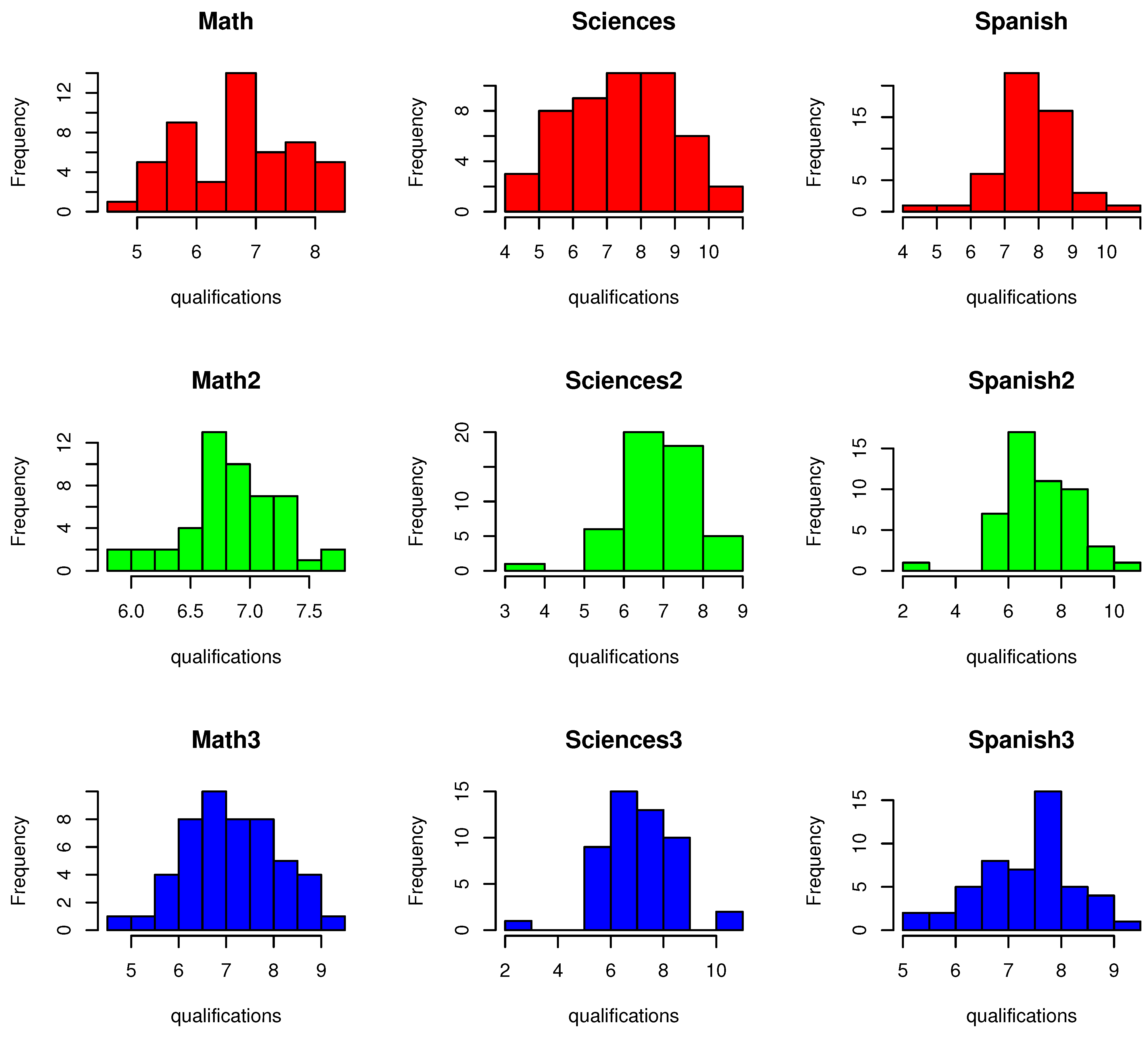
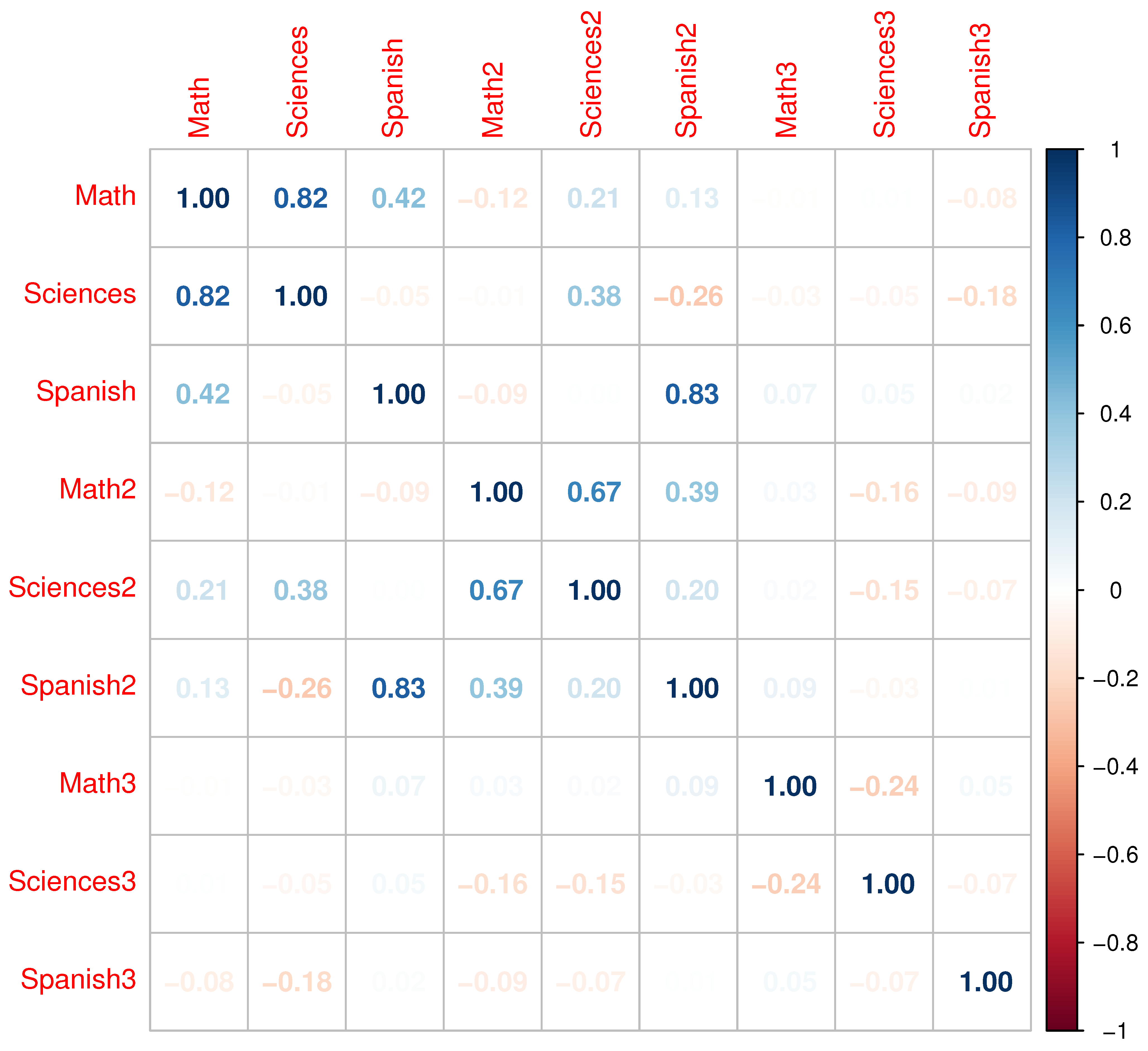
Figure 1 presents a histogram of the qualifications dataset. This first row is related to the first academic period, the second row to the second one, and the third row to the third one. Figure 2 shows the linear correlations between variables, where some correlations higher than 0.6 are highlighted and which are suitable for use in MFA.

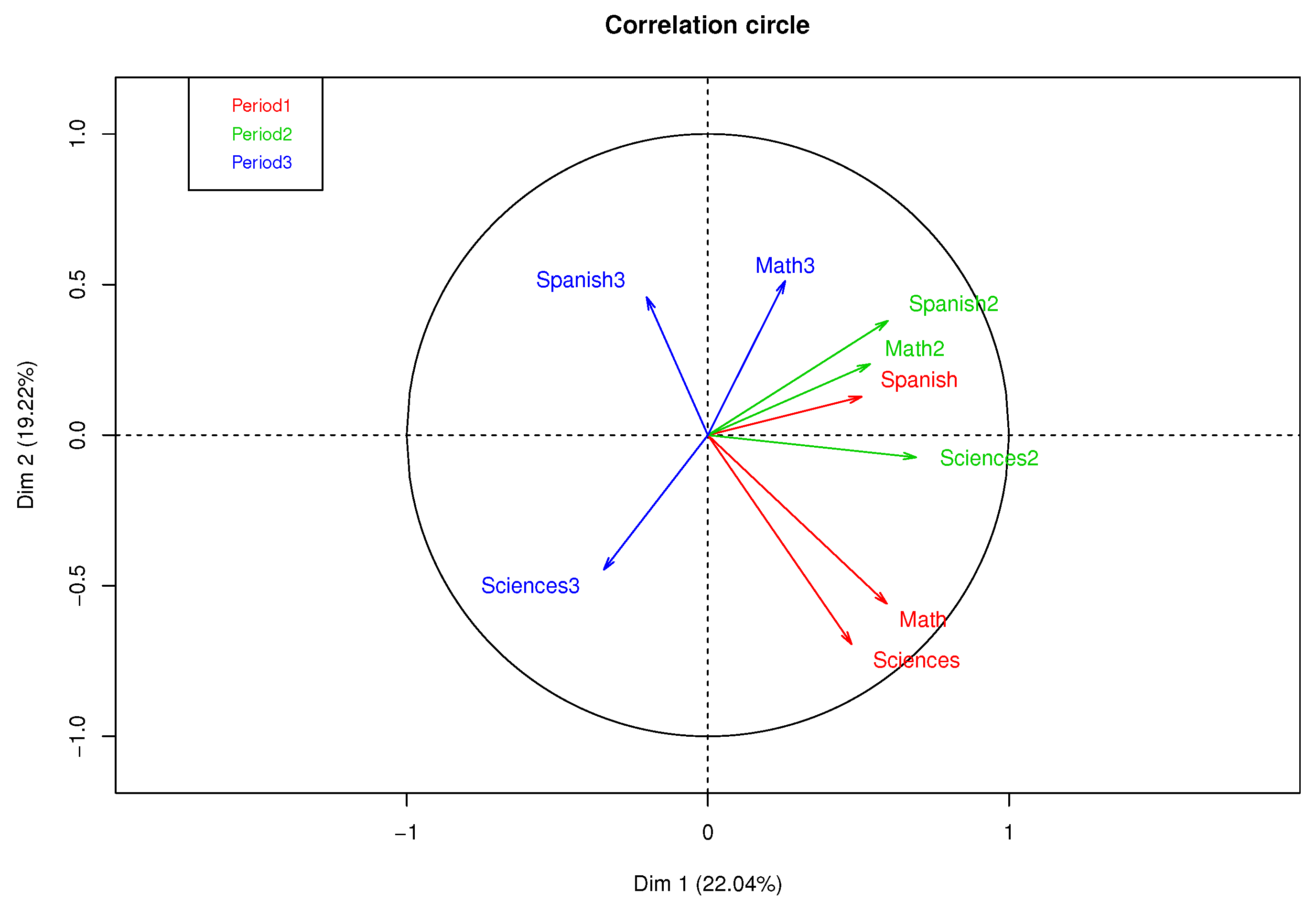
Figure 3 presents a correlation circle of MFA with complete data, where 41.26% of the variance percentage explained was obtained in the first factorial plane. A high correlation between the qualifications of Mathematics and Natural Sciences in the first academic period can be observed, as well as a moderate correlation between Spanish of periods 1 and 2 and a low correlation between subjects in the third period.

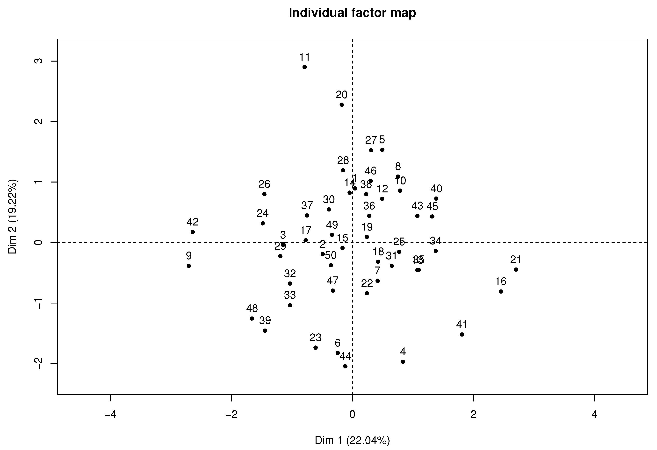
Figure 4 presents the individual factor map where students 11, 21, and 42 highly contribute to the axis, according to their position in the plane far from the average individual or gravity center.

3.1.1. MFA-NIPALS with 10% of NAs

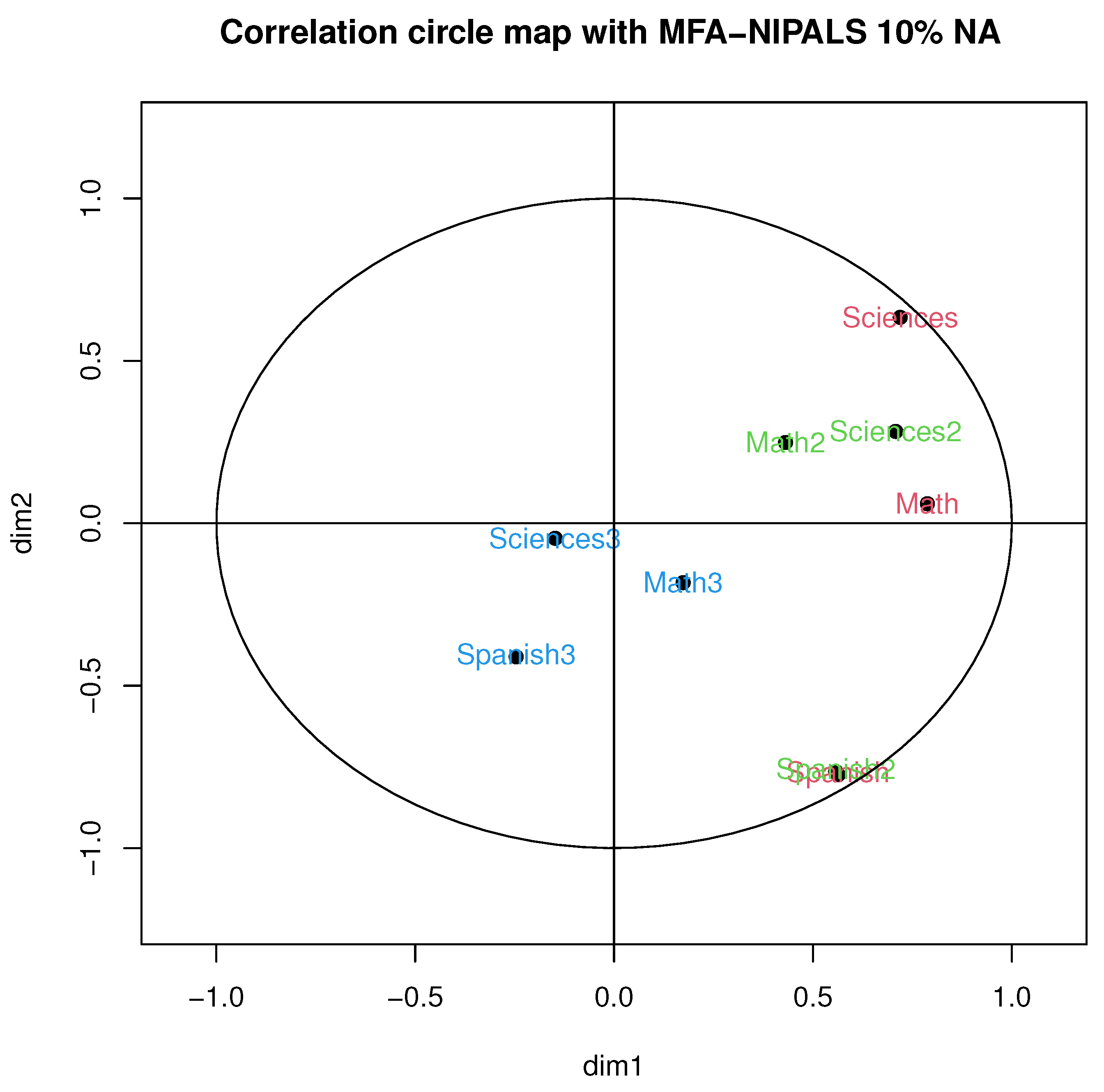
In this section, the main results of the proposed MFA-NIPALS algorithm are presented. Figure 5 illustrates the correlation circle of MFA-NIPALS with 10% of NA. In particular, a high correlation was obtained in periods 1 and 2 with Spanish, as well as a moderate correlation between Mathematics and Natural Sciences in the first academic period and a low correlation between subjects in the third period, which was, for example, observed with MFA with complete data.

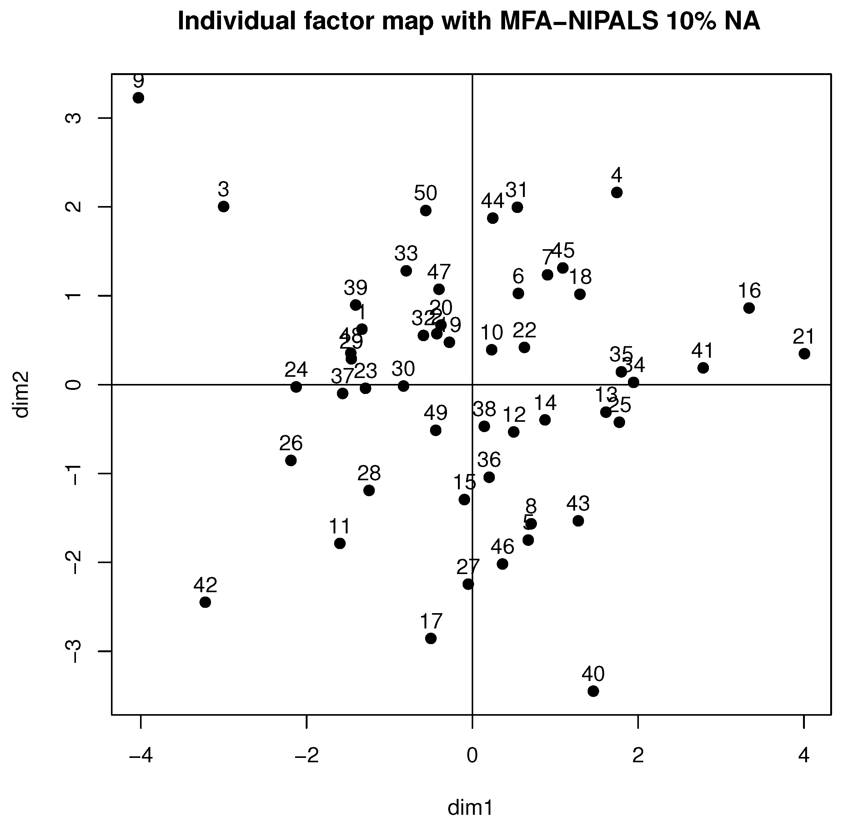
Figure 6 shows the behavior of individuals in the first factorial plane, where similar patterns of a complete data case for students 9, 21, 26, and 42 are highlighted and who highly contributed to the axis, as they are far from the gravity center. Moreover, high variability was detected, which could be produced by the generated NAs of the dataset.

3.1.2. Simulation Scenarios

In this section, results with complete data versus MFA-NIPALS estimates are compared.

Table 2. Percentage of variance explained on axes 1 and 2.

Percentage of NAs	MFA-NIPALS	RIMFA
5%	46.89%	42.46%
10%	50%	43.3%
15%	51.25%	43.66%
20%	56.10%	50.89%
25%	60.41%	53.02%
30%	59.13%	52.24%

shows the percentage of variance explained on axes 1 and 2. These percentages increased when the number of NAs rose. Moreover, the percentages of variance explained by MFA-NIPALS were higher than RIMFA ones, which could be influenced by an increment of eigenvectors on axes 1 and 2. In this comparison, RIMFA holds a percentage of variance explained close to MFA with complete data.

Table 3. Coordinate correlations of individuals for complete data versus NAs on axes 1 and 2.

Axis	Percentage of NAs	MFA-NIPALS	RIMFA
1	5%	0.8789	0.9261
	10%	0.9395	0.9505
	15%	0.9094	0.9527
	20%	0.8920	0.8986
	25%	0.8166	0.7391
	30%	0.7813	−0.0846
2	5%	−0.7918	0.9490
	10%	−0.5490	0.8861
	15%	−0.5773	0.8480
	20%	−0.7214	0.7281
	25%	0.5887	−0.6469
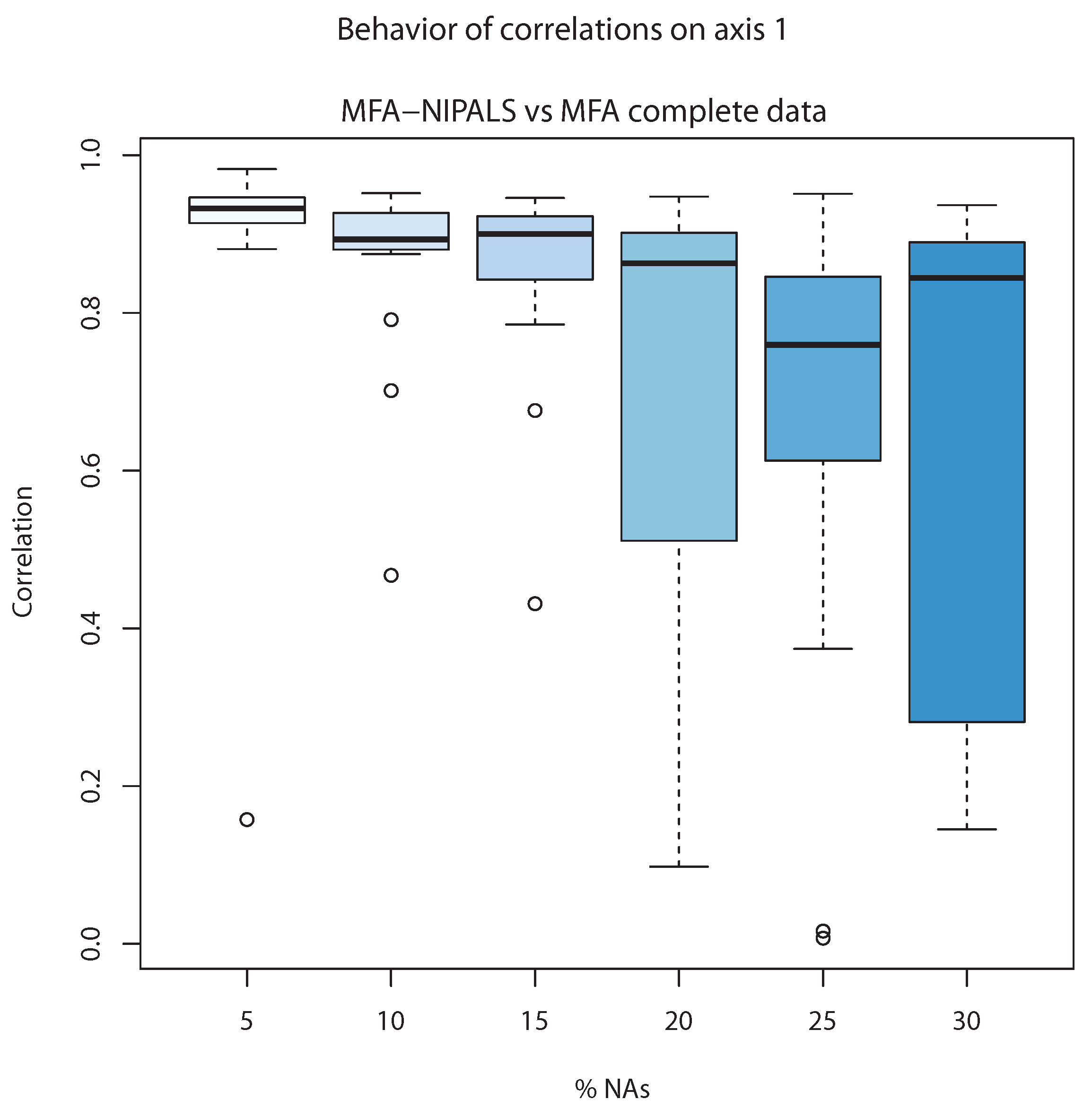
	30%	−0.7494	−0.0027

presents the coordinate correlations with complete data and those estimated by MFA-NIPALS and RIMFA. On axis 1, the highest correlations were detected for MFA-NIPALS and for 30% of NAs, where the RIMFA estimate differed sharply when compared to complete data. For the correlations of axis 2, it can be observed that RIMFA obtained better results than the complete data case. However, a less favorable result was obtained in the case of 30% of NAs.

In summary, MFA-NIPALS performed well on axis 1 and regular on axis 2, indicating that MFA-NIPALS is a good alternative, but more simulation analysis is required to gauge the statistical and computational advantages of MFA-NIPALS versus RIMFA.

Figure 7 shows the correlation between the first component of individuals of classic MFA (${\mathit{\psi }}_1$) and first component of MFA-NIPALS (${\mathit{t}}_1$). The latter analysis was made with 20 matrices randomly generated for several percentages of NAs. When the percentage of NAs increased to 20%, the median of correlations went farther from 1, indicating less correlation between classic MFA and MFA-NIPALS at 20%, 25%, and 30%. Nevertheless, correlation medians until 15% of NAs were closer to 1, indicating that MFA-NIPALS facilitated favorable results based on estimates related to component ${\mathit{t}}_1$.

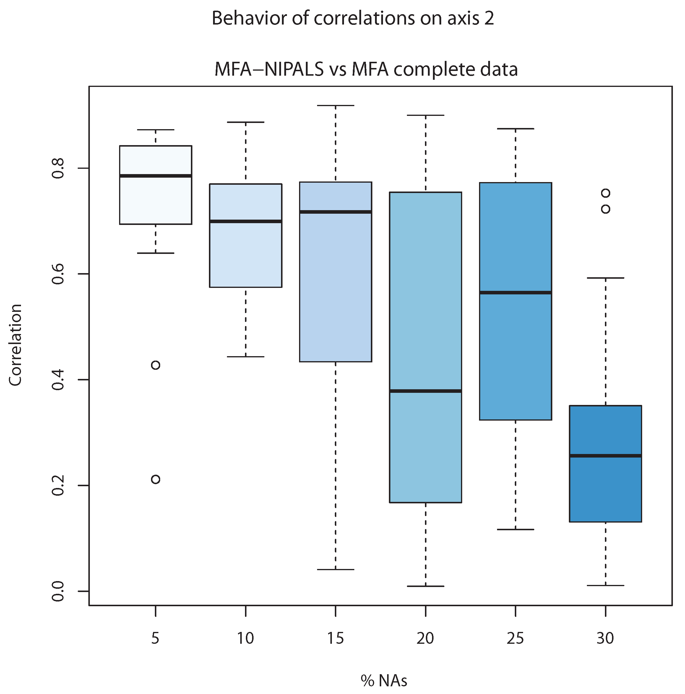
On the other hand, Figure 8 shows the correlation of the second component of classic MFA (${\mathit{\psi }}_2$) and the second component of MFA-NIPALS (${\mathit{t}}_2$). The correlations are close to 0.8 and in cases until 15% of NAs, whereas above 15%, the lowest correlation is observed, indicating that MFA-NIPALS provided a suitable estimation of the second component ${\mathit{t}}_2$ until 15% of NAs.

3.2. Wine Dataset

The wine dataset of the FactoMineR library has $n=21$ observations related to Valle de Loira (France) wines and $p=29$ sensory variables related to wine quality. This dataset contains qualitative and quantitative variables described in [4,39]. For this illustration, we considered quantitative variables. First, we deployed the MFA algorithm for a complete dataset. Additionally, a subset with 7% of NAs of total observations was randomly selected to deploy the RIMFA and MFA-NIPALS algorithms. The results were compared in terms of percentage of explained variance and coordinate correlation of the complete dataset versus RIMFA and MFA-NIPALS algorithms.

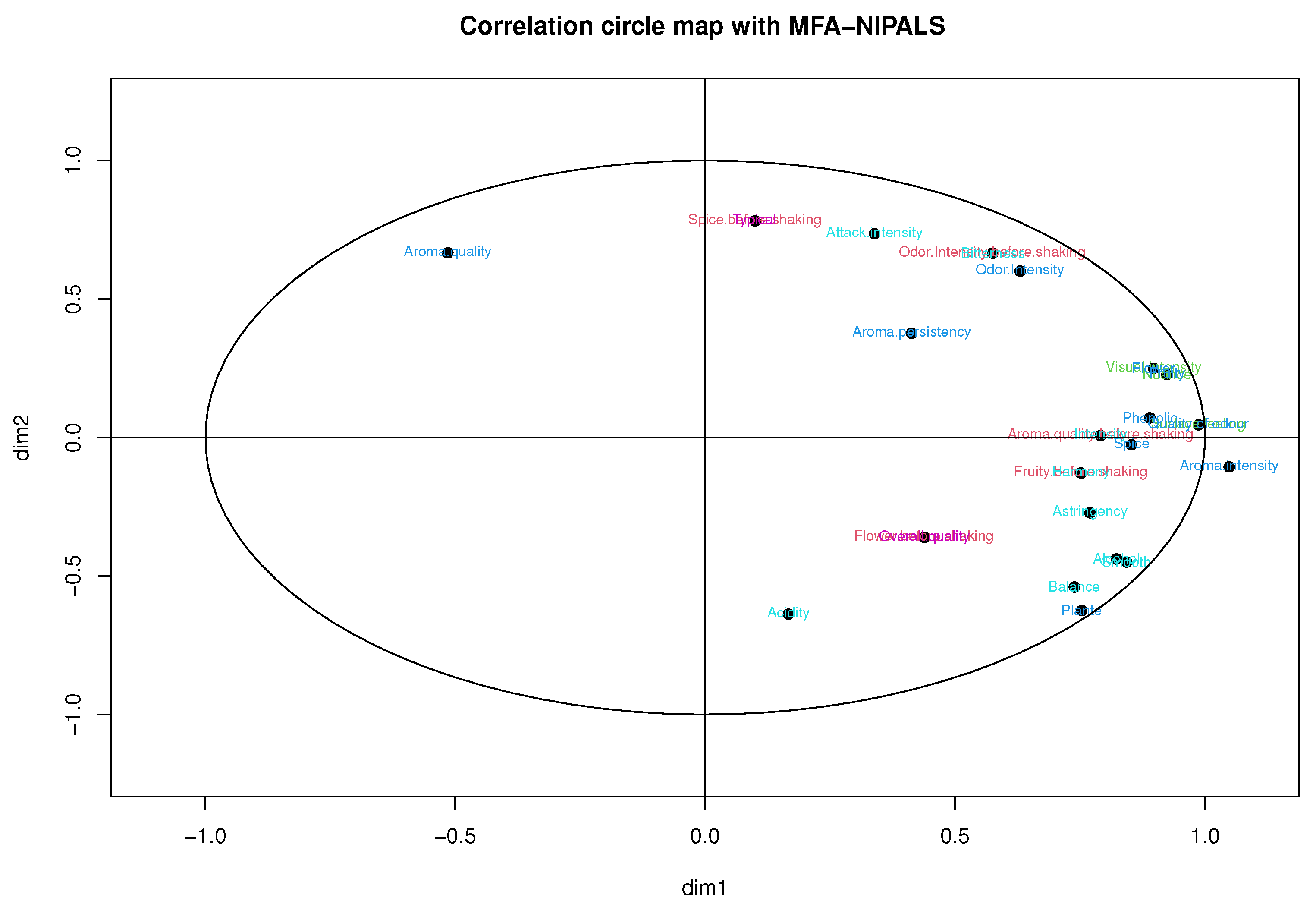
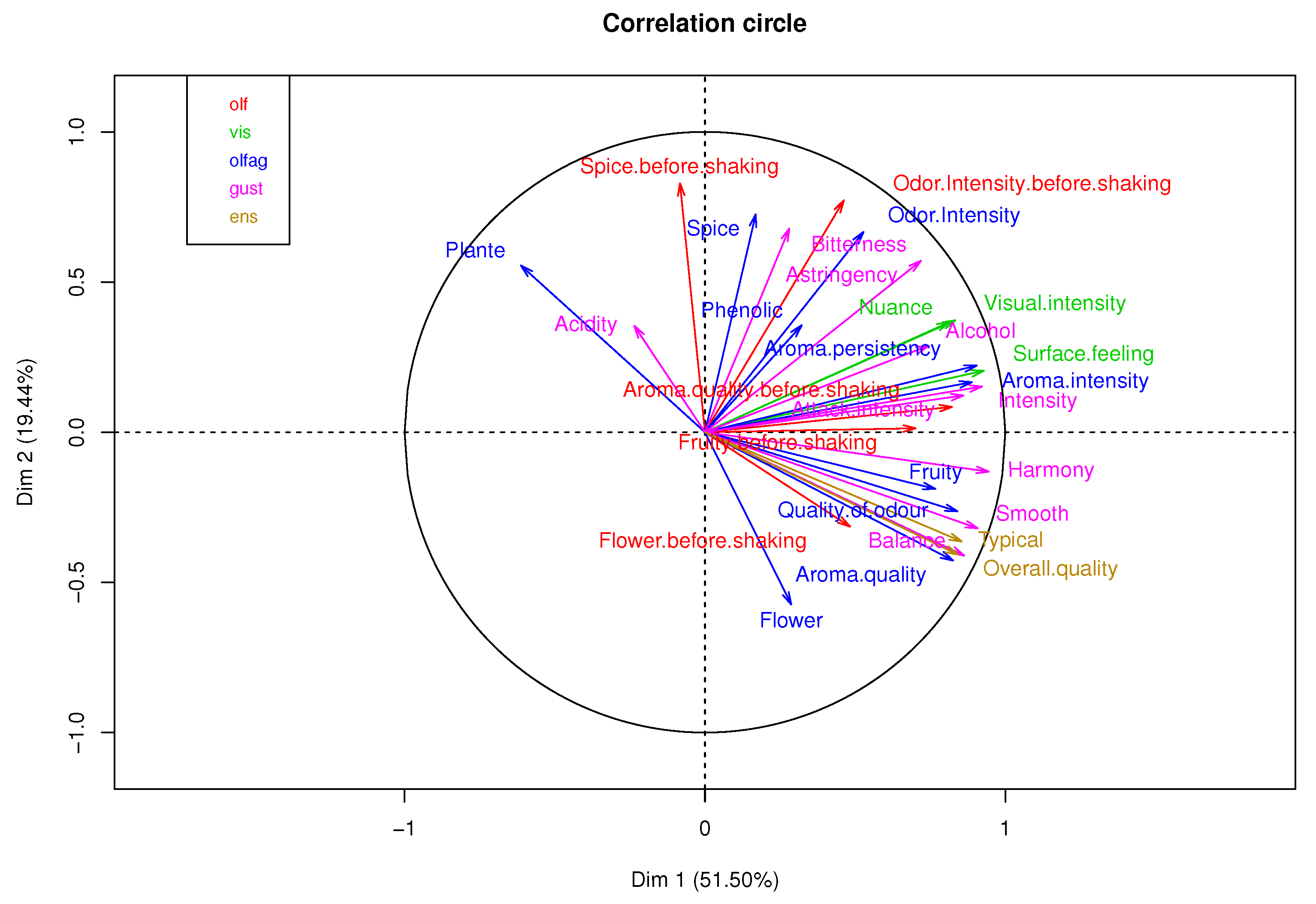
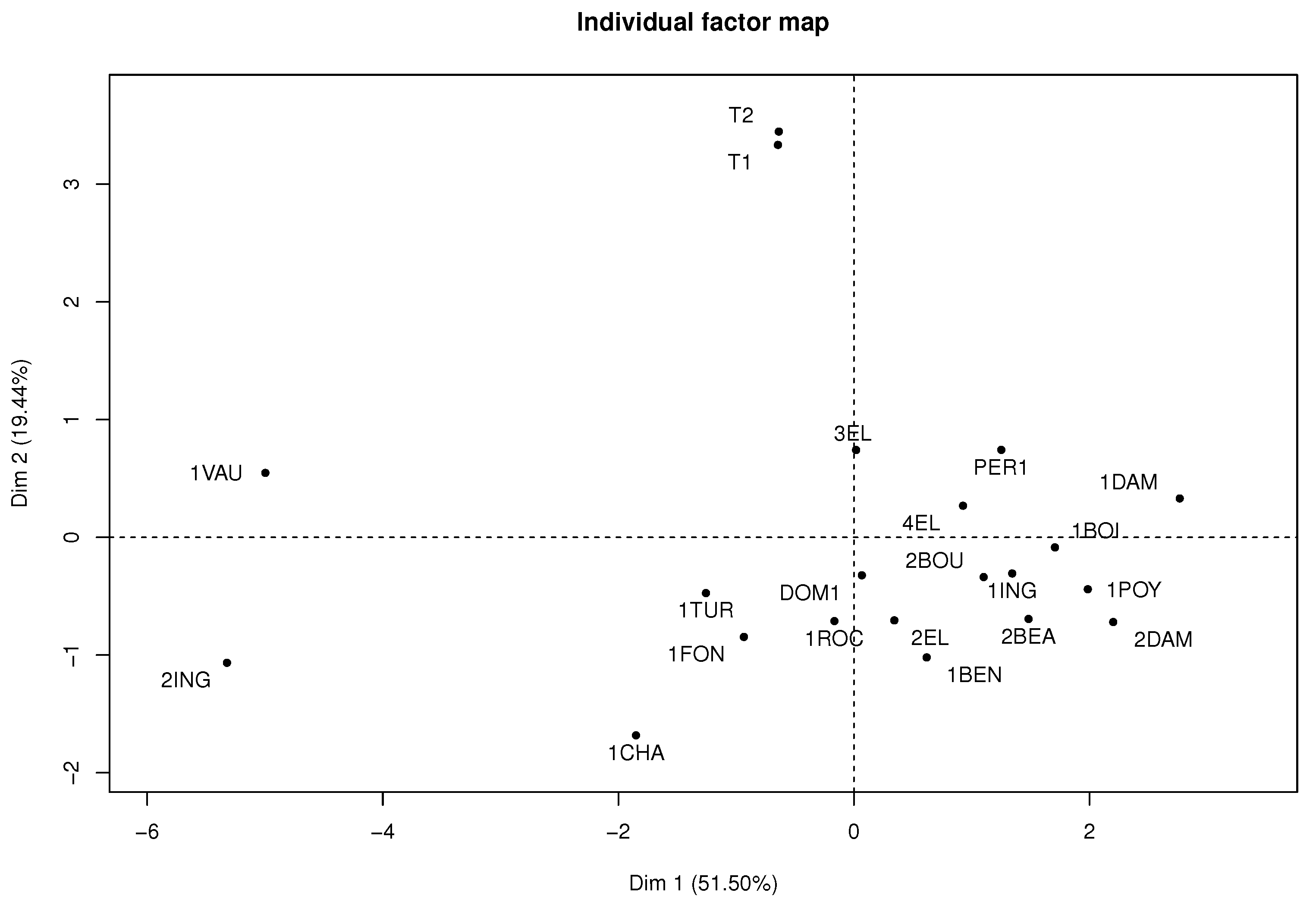
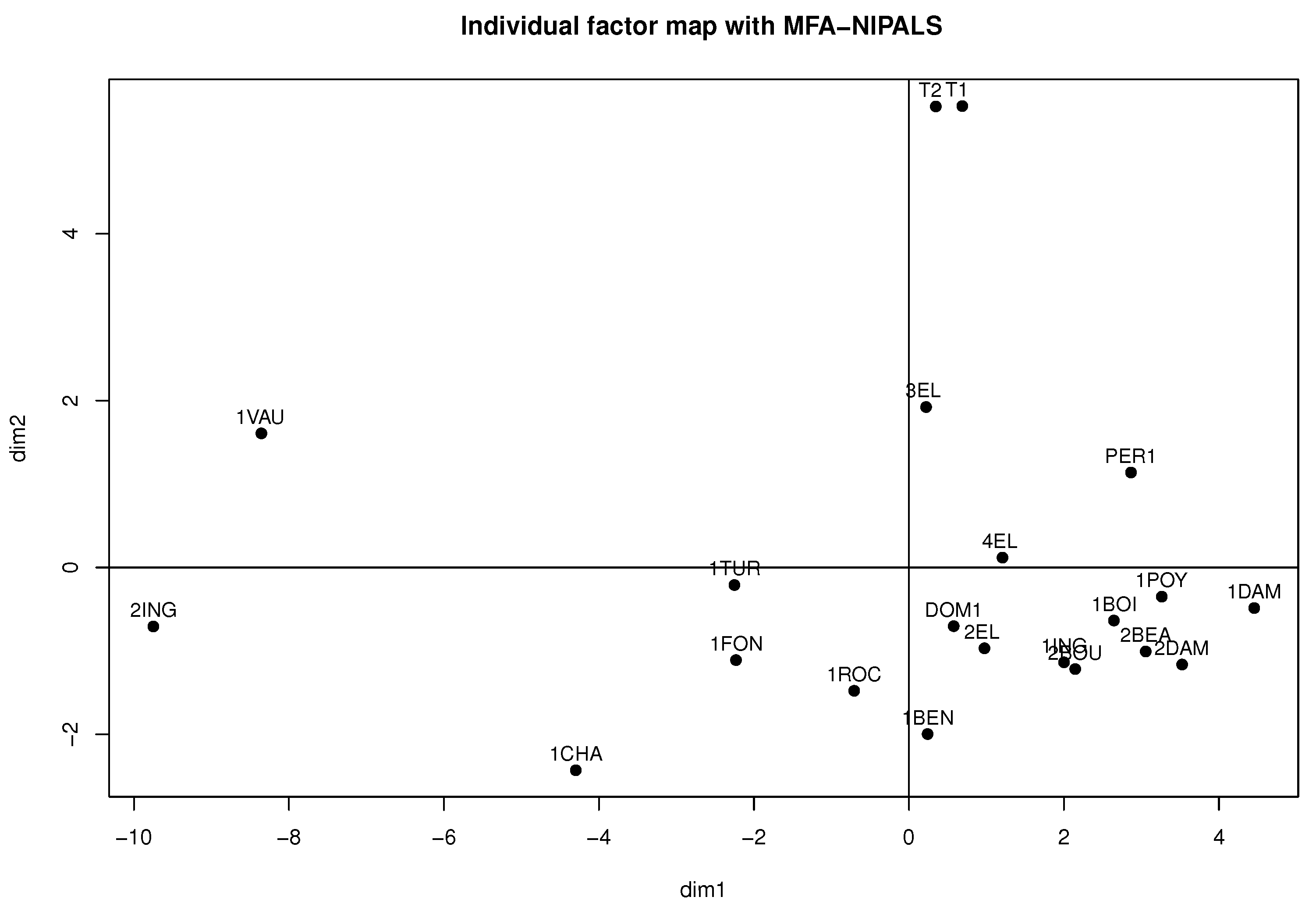
Figure 9 shows the correlation of each table’s variables. The percentage of explained variance in the first two components is 70.94% of the total variability. Figure 10 represents each wine in the factorial plane, where wines T1 and T2 stand out due to similarities of their sensory variables and atypical features. In addition, the 1VAU and 2ING wines are highlighted on the left of the factorial plane, as they presented similarities and atypical features because they differ greatly from the original wines with average features.

Considering Figure 11 and Figure 12, obtained from the MFA-NIPALS algorithm with 7% of NAs, it is evident that the results feature similarities with Figure 9 and Figure 10. Moreover, more similarities for wines in the factorial plane are highlighted. In fact, the correlation between the coordinates of wines from MFA and MFA-NIPALS on the first factorial axis is $cor({\mathit{\psi }}_{\mathbf{1}}MFA,{\mathit{\psi }}_{\mathbf{1}}MFA-NIPALS)=0.9816$ and $cor({\mathit{\psi }}_{\mathbf{2}}MFA,{\mathit{\psi }}_{\mathbf{2}}MFA-NIPALS)=0.9704$ for the second factorial axis. The percentage of explained variance of 72.35%, which is similar to the MFA case with complete dataset, is also highlighted.

For RIMFA, 72.53% of the explained variance was found in the first two factorial axes. Comparing their coordinates versus MFA coordinates using a complete dataset, correlations $cor({\mathit{\psi }}_{\mathbf{1}}MFA,{\mathit{\psi }}_{\mathbf{1}}RIMFA)=0.9985$ and $cor({\mathit{\psi }}_{\mathbf{2}}MFA,{\mathit{\psi }}_{\mathbf{2}}RIMFA)=0.9930$ were found. Thus, the RIMFA algorithm performed better than the MFA-NIPALS one. Nevertheless, MFA-NIPALS performed better than the MFA algorithm in the estimation of coordinates, where $cor({\mathit{\psi }}_{\mathit{MFA}},{\mathit{\psi }}_{\mathit{MFA}-\mathit{NIPALS}})$ is close to 1.

4. Conclusions and Further Works

We successfully coupled the NIPALS algorithm with MFA for missing data, called the MFA-NIPALS algorithm. The proposed algorithm was implemented with R software and an alternative method for data imputation with RIMFA was configured. MFA-NIPALS was adapted using the nipals function of the ade4 library. Other options such as the nipals function of the plsdepot library [42] could be explored. Karimov et al. [43] considered phase space reconstruction techniques mainly oriented toward classification tasks, where the integrate-and-differentiate approach is focused on improving identification accuracy through the elimination of classification errors needed for the parameter estimation of nonlinear equations. Further studies could explore the integrate-and-differentiate approach regarding the missing data problem.

Further works could analyze if Gram–Schmidt orthogonalization helps to find better properties for MFA-NIPALS. The literature contains multiple factorial methods, in which the missing data problem has not been addressed with NIPALS, for example, the STATIS-ACT method and canonical correlation analysis (ACC) [44,45]. The NIPALS algorithm seems suitable to address missing data in STATIS-ACT and ACC.

Another important concept related to MFS is the RV coefficient of Escoufier [46,47], which is a matrix version of the Pearson coefficient of correlation. The RV coefficient between tables $X_{n\times p}$ and $Y_{n\times q}$ is:

$$RV(\mathit{X},\mathit{Y})=\frac{tr\left\{\mathit{X}{\mathit{X}}^{\top }\mathit{Y}{\mathit{Y}}^{\top }\right\}}{tr\left\{\mathit{X}{\mathit{X}}^{\top }\mathit{X}{\mathit{X}}^{\top }\right\}tr\left\{\mathit{Y}{\mathit{Y}}^{\top }\mathit{Y}{\mathit{Y}}^{\top }\right\}},$$

(18)

where $tr\left\{\mathit{A}\right\}$ denotes the trace of matrix $\mathit{A}$ [36].

The RV coefficient is often used to study the correlation between tables or groups of variables. The coefficients related to the covariance of a pair of tables appear in the numerator of (18). If X and Y include NAs and MFA-NIPALS is used, further work could focus on RV coefficient computation using the available data principle (see Section 2.4). Another proposal is the use of coordinates between individuals ${\mathit{\psi }}^{\left(k\right)}$ in the kth table as an estimation of X and Y, since coordinates ${\mathit{\psi }}^{\left(k\right)}$ do not have NAs when MFA-NIPALS is deployed.

In this paper, MFA-NIPALS was used for longitudinal quantitative variables with the presence of NAs. This approach could be extended to multiple k qualitative tables using MCA under the available data principle [19]. This idea allows working with MFA-NIPALS with mixed data using NIPALS for quantitative tables and MCA for qualitative ones. Given that the available data principle reduces computational cost when MFA-NIPALS is used compared to RIMFA, the MFA-NIPALS algorithm is a novel approach to addressing missing data problems in multiple quantitative tables. Nevertheless, further studies are needed to compare MFA-NIPALS with RIMFA across datasets with higher dimensions, analyzing the computational performance of both methods by comparing the estimated coordinates of $\mathit{\psi }$ (in presence of NAs) with MFA coordinates (of a complete dataset). It is expected that MFA-NIPALS performs better with datasets with more variables than observations ($p>n$), where PLS methods have advantages over classic methods [48].

Based on simulation scenarios, it is recommended to work the MFA-NIPALS proposal until 15% of NAs of the total number of observations. This result is in line with the results by [24], highlighting the NAs percentage recommended for NIPALS. Moreover, it is recommended to use MFA-NIPALS when data imputation is not feasible. Though the RIMFA algorithm performed well when coordinates are compared to the MFS one, this study showed that the MFA-NIPALS algorithm was a good alternative for NA handling in the MFA. Moreover, our proposal is promising, as it yielded favorable results regarding the percentage of explained variance. It is highly probable that other studies generate even better results by mixing the MFA-NIPALS and RIMFA approaches.

References

1. Aluja-Banet, T.; Morineau, A. Aprender de Los Datos: El análisis de Componentes Principales: Una Aproximación Desde El Data Mining; Number Sirsi i9788483120224; Ediciones Universitarias de Barcelona: Barcelona, Spain, 1999. [Google Scholar]
2. Lebart, L.; Morineau, A.; Piron, M. Statistique Exploratoire Multidimensionnelle; Dunod: Paris, France, 1995; Volume 3. [Google Scholar]
3. Escofier, B.; Pages, J. Multiple Factor Analysis (AFMULT Package). Comput. Stat. Data Anal. 1994, 18, 121–140. [Google Scholar] [CrossRef]
4. Escofier, B.; Pagès, J. Analyses Factorielles Simples et Multiples; Dunod: Paris, France, 1998; Volume 284. [Google Scholar]
5. Abdi, H.; Williams, L.J.; Valentin, D. Multiple factor analysis: Principal component analysis for multitable and multiblock data sets. Wiley Interdiscip. Rev. Comput. Stat. 2013, 5, 149–179. [Google Scholar] [CrossRef]
6. Ochoa-Muñoz, A.F.; Peña-Torres, J.A.; García-Bermúdez, C.E.; Mosquera-Muñoz, K.F.; Mesa-Diez, J. On characterization of sensory data in presence of missing values: The case of sensory coffee quality assessment. INGENIARE-Rev. Chil. De Ing. 2022, 30. [Google Scholar] [CrossRef]
7. Corzo, J.A. Análisis factorial múltiple para clasificación de universidades latinoamericanas. Comun. En Estadística 2017, 10, 57–82. [Google Scholar] [CrossRef]
8. Cadavid-Ruiz, N.; Herrán-Murillo, Y.F.; Patiño-Gil, J.C.; Ochoa-Muñoz, A.F.; Varela-Arévalo, M.T. Actividad física y percepción de bienestar en la universidad: Estudio longitudinal durante el COVID-19 (Physical activity and perceived well-being at the university: Longitudinal study during COVID-19). Retos 2023, 50, 102–112. [Google Scholar] [CrossRef]
9. Van Buuren, S. Flexible Imputation of Missing Data; CRC Press: Boca Raton, FL, USA, 2018. [Google Scholar]
10. Song, S.; Sun, Y.; Zhang, A.; Chen, L.; Wang, J. Enriching data imputation under similarity rule constraints. IEEE Trans. Knowl. Data Eng. 2018, 32, 275–287. [Google Scholar] [CrossRef]
11. Little, R.J.; Rubin, D.B. Statistical Analysis with Missing Data; John Wiley & Sons: Hoboken, NJ, USA, 2019; Volume 793. [Google Scholar]
12. Breve, B.; Caruccio, L.; Deufemia, V.; Polese, G. RENUVER: A Missing Value Imputation Algorithm based on Relaxed Functional Dependencies. In Proceedings of the EDBT, Edinburgh, UK, 29 March–1 April 2022; pp. 1–52. [Google Scholar]
13. Husson, F.; Josse, J. Handling missing values in multiple factor analysis. Food Qual. Prefer. 2013, 30, 77–85. [Google Scholar] [CrossRef]
14. Josse, J.; Husson, F. missMDA: A package for handling missing values in multivariate data analysis. J. Stat. Softw. 2016, 70, 1–31. [Google Scholar] [CrossRef]
15. Josse, J.; Husson, F. Gestion des données manquantes en analyse en composantes principales. J. Société Française Stat. 2009, 150, 28–51. [Google Scholar]
16. Wold, H. Estimation of principal components and related models by iterative least squares. Multivar. Anal. 1966, 1, 391–420. [Google Scholar]
17. Wold, H. Nonlinear iterative partial least squares (NIPALS) modelling: Some current developments. In Multivariate Analysis–III; Elsevier: Amsterdam, The Netherlands, 1973; pp. 383–407. [Google Scholar]
18. Gonzalez-Rojas, V.; Conde-Arango, G.; Ochoa-Muñoz, A. Análisis de Componentes Principales en presencia de datos faltantes: El principio de datos disponibles. Sci. Tech. 2021, 26, 210–228. [Google Scholar] [CrossRef]
19. Ochoa-Muñoz, A.F.; González-Rojas, V.M.; Pardo, C.E. Missing data in multiple correspondence analysis under the available data principle of the NIPALS algorithm. Dyna 2019, 86, 249–257. [Google Scholar] [CrossRef]
20. González-Rojas, V. Inter-battery factor analysis via pls: The missing data case. Rev. Colomb. Estad. 2016, 39, 247–266. [Google Scholar] [CrossRef]
21. Patel, N.; Mhaskar, P.; Corbett, B. Subspace based model identification for missing data. AIChE J. 2020, 66, e16538. [Google Scholar] [CrossRef]
22. Preda, C.; Saporta, G.; Mbarek, M.H. The NIPALS algorithm for missing functional data. Rev. Roum. Math. Pures Appli. 2010, 55, 315–326. [Google Scholar]
23. Canales, T.M.; Lima, M.; Wiff, R.; Contreras-Reyes, J.E.; Cifuentes, U.; Montero, J. Endogenous, climate, and fishing influences on the population dynamics of small pelagic fish in the southern Humboldt current ecosystem. Front. Mar. Sci. 2020, 7, 82. [Google Scholar] [CrossRef]
24. Tenenhaus, M. La Régression PLS, Théorie et Pratique; Editions Technip: Paris, France, 1998. [Google Scholar]
25. González Rojas, V.M. Análisis conjunto de múltiples tablas de datos mixtos mediante PLS. Ph.D. Thesis, Universitat Politécnica de Catalunya, Barcelona, Spain, 2014. [Google Scholar]
26. Krämer, N. Analysis of High Dimensional Data with Partial Least Squares and Boosting. Ph.D. Thesis, Technischen Universität Berlin, Berlin, Germany, 2007. [Google Scholar]
27. Alin, A. Comparison of PLS algorithms when number of objects is much larger than number of variables. Stat. Pap. 2009, 50, 711–720. [Google Scholar] [CrossRef]
28. Abdi, H.; Valentin, D. Multiple factor analysis (MFA). Encycl. Meas. Stat. 2007, II, 657–663. [Google Scholar]
29. Pardo, C.E. Métodos en ejes principales para tablas de contingencia con estructuras de participación en filas y columnas. Ph.D. Thesis, Universidad Nacional de Colombia, Bogotá, Colombia, 2010. [Google Scholar]
30. Josse, J.; Husson, F. Handling missing values in exploratory multivariate data analysis methods. J. Société Française Stat. 2012, 153, 79–99. [Google Scholar]
31. Josse, J.; Chavent, M.; Liquet, B.; Husson, F. Handling missing values with regularized iterative multiple correspondence analysis. J. Classif. 2012, 29, 91–116. [Google Scholar] [CrossRef]
32. Josse, J.; Husson, F. Selecting the number of components in principal component analysis using cross-validation approximations. Comput. Stat. Data Anal. 2012, 56, 1869–1879. [Google Scholar] [CrossRef]
33. Vega-Vilca, J.C.; Guzmán, J. Regresión PLS y PCA como solución al problema de multicolinealidad en regresión múltiple. Rev. De Mat. Teoría Y Apl. 2011, 18, 9–20. [Google Scholar] [CrossRef]
34. Vicente-Gonzalez, L.; Vicente-Villardon, J.L. Partial Least Squares Regression for Binary Responses and Its Associated Biplot Representation. Mathematics 2022, 10, 2580. [Google Scholar] [CrossRef]
35. Contreras-Reyes, J.E. Mutual information matrix based on asymmetric Shannon entropy for nonlinear interactions of time series. Nonlinear Dyn. 2021, 104, 3913–3924. [Google Scholar] [CrossRef]
36. Contreras-Reyes, J.E. Mutual information matrix based on Rényi entropy and application. Nonlinear Dyn. 2022, 110, 623–633. [Google Scholar] [CrossRef]
37. Trejos-Zelaya, J.; Castillo-Elizondo, W.; Gónzalez-Varela, J. Análisis Multivariado de Datos: Métodos y Aplicaciones; UCR: Riverside, CA, USA, 2014. [Google Scholar]
38. Ochoa-Muñoz, A.F. Ejemplo 1-AFM Diplomado; Technical Report; Universidad del Valle: Cali, Colombia, 2020. [Google Scholar]
39. Lê, S.; Josse, J.; Husson, F. FactoMineR: An R package for multivariate analysis. J. Stat. Softw. 2008, 25, 1–18. [Google Scholar] [CrossRef]
40. Husson, F.; Josse, J.; Le, S.; Mazet, J.; Husson, M.F. Package ‘factominer’. R Package 2016, 96, 698. [Google Scholar]
41. Dray, S.; Siberchicot, M.A. Package ‘ade4’; Université de Lyon: Lyon, France, 2017. [Google Scholar]
42. Sanchez, G.; Sanchez, M.G. Package ‘plsdepot’. In Partial Least Squares (PLS) Data Anal. Methods, V. 0.1; Université de Technologie de Troyes: Troyes, Grand-Est, France, 2012; Volume 17. [Google Scholar]
43. Karimov, A.I.; Kopets, E.; Nepomuceno, E.G.; Butusov, D. Integrate-and-differentiate approach to nonlinear system identification. Mathematics 2021, 9, 2999. [Google Scholar] [CrossRef]
44. Lavit, C.; Escoufier, Y.; Sabatier, R.; Traissac, P. The act (statis method). Comput. Stat. Data Anal. 1994, 18, 97–119. [Google Scholar] [CrossRef]
45. Thompson, B. Canonical Correlation Analysis: Uses and Interpretation; Sage: California, CA, USA, 1984. [Google Scholar]
46. Escoufier, Y. Le traitement des variables vectorielles. Biometrics 1973, 29, 751–760. [Google Scholar] [CrossRef]
47. Josse, J.; Pagès, J.; Husson, F. Testing the significance of the RV coefficient. Comput. Stat. Data Anal. 2008, 53, 82–91. [Google Scholar] [CrossRef]
48. Vitelleschi, M.S. Modelos PCA a partir de conjuntos de datos con información faltante:¿ Se afectan sus propiedades? SaberEs 2010, 2, 105–109. [Google Scholar] [CrossRef]
Figure 1. Histogram of qualifications for the three academic periods.
Algorithms 16 00457 g001
Figure 2. Correlation matrix of qualifications for the three academic periods.
Algorithms 16 00457 g002
Figure 3. Correlation circle of MFA with complete data.
Algorithms 16 00457 g003
Figure 4. Individual factor map of MFA with complete data.
Algorithms 16 00457 g004
Figure 5. Correlation circle of MFA-NIPALS algorithm with 10% of NAs.
Algorithms 16 00457 g005
Figure 6. Individual factor map of MFA-NIPALS algorithm with 10% of NAs.
Algorithms 16 00457 g006
Figure 7. Correlation of complete data versus MFA-NIPALS with NAs on axis 1.
Algorithms 16 00457 g007
Figure 8. Correlation of complete data versus MFA-NIPALS with NAs on axis 2.
Algorithms 16 00457 g008
Figure 9. Correlation circle of MFA algorithm in wine dataset.
Algorithms 16 00457 g009
Figure 10. Individual factor map of MFA algorithm in wine dataset.
Algorithms 16 00457 g010
Figure 11. Correlation circle of MFA-NIPALS algorithm with 7% of NAs in wine dataset.
Algorithms 16 00457 g011
Figure 12. Individual factor map of MFA algorithm with 7% of NAs in wine dataset.
Algorithms 16 00457 g012