Solving of the Inverse Boundary Value Problem for the Heat Conduction Equation in Two Intervals of Time

Abstract

The boundary value problem, BVP, for the PDE heat equation is studied and explained in this article. The problem declaration comprises two intervals; the (0, T) is the first interval and labels the heating of the inside burning chamber, and the second (T, ∞) interval defines the normal cooling of the chamber wall when the chamber temperature concurs with the ambient temperature. It is necessary to prove the boundary function of this problem has its place in the space $H^1\left[0,\infty \right]$ in order to successfully apply the Fourier transform method. The applicability of the Fourier transform for time to this problem is verified. The method of projection regularization is used to solve the inverse boundary value problem for the heat equation and to obtain an evaluation for the error between the approximate and the real solution. These results are new and of practical interest as shown in the numerical case study.

1. Introduction

A heat speared problem handles the estimate of unidentified numbers appearing in the mathematics of physical in thermal knowledges, by means of the dimensions or measurement of the temperature, radiation intensities, heat flux, etc.

The inverse problem for the heat PDE system can be solved by many methods; for example, the method of Tikhonov [1], the method of Lavrentiev [2], Ivanov [3], and many others. The inverse problems in the heat PDE system can be grouped as two types depending on the e unknown function or vector for the initial part or the boundary part conditions, and many studies of these problems are considered in many works [4,5,6,7,8,9,10,11,12]. Various methods for solving this type of inverse problem have been proposed in many works [13,14,15,16,17]. In the article [13], the BVP for the PDE heat equation in a hollow cylinder was solved by using the Fourier projection method. Papers [14,16] studied the multigrid method with the iterative method to find the solution for the inverse problem, IP, in the heat PDE system. In [15,17], the iterative methods with necessary analyses were studied for solving the inverse linear operator equation and the case study in this paper was the inverse heat PDE system problem.

The successfully accomplished approaches for resolving the IPs are dependent, to a large degree, on the deep insight into the mathematical problems related to the algorithms and statements and the definition of the specific difficulties in their solving [18,19,20,21,22,23].

The goal of this article is to provide the approximation solution for the BVP in the PDE for the heat equation system with the mixed interval for time. Hence, the result of this problem (BVP) is not contingent continuously on the known data in the field, which means the solution is not stable; therefore, this problem is known as an ill-posed inverse problem. The proving of the boundary function of this problem belonged to the class $H^1\left[0,\infty \right]$ necessary for applying the projection regularization method by using the Fourier transform. For solving the ill-posed problems, a central role is played by the error estimations between the approximation and real solutions. We obtain the estimate solution by applying the projection regularization method with the Fourier transform, making these results new and interesting.

2. Materials and Methods Direct Formulation of the Problem on Interval $\left(\mathbf{0}\mathbf{,}\mathit{T}\right]$

We considered the case of the heat equation on a segment with inhomogeneous boundary data.

$$\frac{\partial u_1\left(x,t\right)}{\partial t}=\frac{{\partial }^2{u}_1\left(x,t\right)}{\partial x^2},0<x<1,t\in \left(0,T\right],$$

(1)

$$u_1\left(x,0\right)=0,0\le x\le 1,$$

(2)

$$u_1\left(0,t\right)=0,0\le t\le T,$$

(3)

$$u_1\left(1,t\right)=u\left(t\right),0\le t\le T,$$

(4)

Assume the $q\left(t\right)$ function is defined as the following

$$q_1\left(t\right)\in C^3\left[0,T\right],q_1\left(0\right)={q^{\prime }}_1\left(0\right)={q^{″}}_1\left(0\right)={q^{\prime }}_1\left(T\right)={q^{″}}_1\left(T\right)=0,$$

(5)

by using Duhamel’s principle method ([24], p. 109)

$$u_1(x,t)={\displaystyle \underset{0}{\overset{t}{\int }}{w}_t(x,t-\tau )q_1(\tau )d\tau ,}$$

(6)

integration by parts for the right part for (6) once, we obtain

$$u_1(x,t)={\displaystyle \underset{0}{\overset{t}{\int }}w(x,t-\tau ){q^{\prime }}_1(\tau )d\tau +q_1(0)w(x,t)}.$$

(7)

Now, we can decide to obtain the solution for $w(x,t)$ as the following

$$w(x,t)=x+2{\displaystyle \sum _{n=1}^{\infty }\frac{{\left(-1\right)}^n}{n\pi }{e}^{-{(n\pi )}^{2}t}\sin (n\pi x)},$$

(8)

by substituting (8) in (7), to obtain a solution to a non-stationary problem, from (5) $q_1\left(0\right)=0,$

$$u_1(x,t)=x+{\displaystyle \sum _{n=1}^{\infty }{\left(-1\right)}^n{C}_n(t)\sin (n\pi x)},$$

(9)

$$C_n(t)=\frac{2}{n\pi }{\displaystyle \underset{0}{\overset{t}{\int }}{e}^{-{(n\pi )}^2(t-\tau )}{q^{\prime }}_1(\tau )d\tau },$$

(10)

where $x\in \left(0,1\right)$, and $t\in \left(0,T\right].$

Lemma 1.

Let$q_1(t)$satisfy condition (5). Then, there exists a solution$u_1(x,t)$for problem (1)–(5) such that$u_1(x,t)$satisfies the Equation (1) on the set$\left(0,1\right)\times \left(0,T\right]$, initial condition (2), boundary conditions (3), (4) and$u_1\left(x,t\right)\in C\left(\left[0,1\right]\times \left[0,T\right]\right)\cap C^{2,1}\left(\left(0,1\right)\times \left(0,T\right]\right).$

Proof. 

By integrating the right side of the Formula (10) in parts twice, we obtain

$$C_n(t)=\frac{2}{{\left(n\pi \right)}^5}{\displaystyle \underset{0}{\overset{t}{\int }}{e}^{-{(n\pi )}^2(t-\tau )}{q^{‴}}_1(\tau )d\tau }+\frac{2}{{\left(n\pi \right)}^3}{q^{\prime }}_1(t)-\frac{2}{{\left(n\pi \right)}^5}{q^{″}}_1(t),$$

(11)

since $\left|C_n(t)\sin (n\pi x)\right|\le \left|C_n(t)\right|$ for any $n$ and from the Cauchy–Bunyakovsky inequality

$$\left|{\displaystyle \underset{0}{\overset{t}{\int }}{e}^{-{(n\pi )}^2(t-\tau )}{q^{‴}}_1(\tau )d\tau }\right|\le {‖{q^{‴}}_1(\tau )‖}_{L_2(0,T]}\frac{1}{\sqrt{2}n\pi },$$

(12)

by means of (5), (4) and (12) for any $t\in \left(0,T\right]$ and for any $n$ we obtain

$$\left|C_n(t)\right|\le \frac{\sqrt{2}{‖{q^{‴}}_1(t)‖}_{L_2}}{{\left(n\pi \right)}^6}+\frac{2}{{\left(n\pi \right)}^3}{q^{\prime }}_1(t)-\frac{2}{{\left(n\pi \right)}^5}{q^{″}}_1(t).$$

(13)

Using Equations (11)–(13) and convergence of the series ${\displaystyle \sum _{n-1}^{\infty }\frac{1}{n^3}}$, ${\displaystyle \sum _{n-1}^{\infty }\frac{1}{n^5}}$, ${\displaystyle \sum _{n-1}^{\infty }\frac{1}{n^6}}$ with the Weierstrass criterion follows the unchanging convergence of the above series on $\left(0,1\right)\times \left(0,T\right]$.

Since the functions $e^{-{(n\pi )}^2(\tau )}{q^{‴}}_1(\tau )\in L_2\left(0,T\right]$, obtaining

$${\displaystyle \underset{0}{\overset{t}{\int }}{e}^{-{(n\pi )}^2(t-\tau )}{q^{‴}}_1(\tau )d\tau }=e^{-{(n\pi )}^{2}t}{\displaystyle \underset{0}{\overset{t}{\int }}{e}^{{(n\pi )}^2\tau }{q^{‴}}_1(\tau )d\tau }\in C\left(0,T\right].$$

(14)

Thus, with $q_1(t),{q^{\prime }}_1(t)$ and ${q^{″}}_1(t)\in C\left(0,T\right]$ in addition to Equations (11) and (14), we take $C_n(t)\in C\left(0,T\right]$. From this condition and the convergence of (19) in domain $\left(0,1\right)\times \left(0,T\right]$, we have $u_1(x,t)\in C(\left(0,1\right)\times \left(0,T\right])$. Differentiating a $C_n(t)\sin (n\pi x)$ with $x$ and by using (13), we obtain

$$\left|{\left(C_n(t)\sin n\pi x\right)}^{\prime }{}_x\right|\le \frac{\sqrt{2}{‖{q^{‴}}_1(t)‖}_{L_2}}{{\left(n\pi \right)}^5}+\frac{2}{{\left(n\pi \right)}^3}{q^{\prime }}_1(t)-\frac{2}{{\left(n\pi \right)}^4}{q^{″}}_1(t).$$

From the above relation, we obtain the convergence of the ${\displaystyle \sum _{n-0}^{\infty }{\left(C_n(t)\sin n\pi x\right)}^{\prime }{}_x}$ in $\left[0,1\right]\times \left[0,T\right]$, from (8) we have $\frac{\partial u_1(x,t)}{\partial x}={\displaystyle \sum _{n-0}^{\infty }{\left(C_n(t)\sin n\pi x\right)}^{\prime }{}_x}$ in $\left(0,1\right)\times \left(0,T\right]$ and $\frac{\partial u_1(x,t)}{\partial x}\in (\left(0,1\right)\times \left(0,T\right])$.

Now, let us examine the function $\frac{{\partial }^2{u}_1(x,t)}{\partial x^2}$.

Differentiating the function $C_n(t)\sin (n\pi x)$ by $x$ twice and using (11), we obtain ${\left(C_n(t)\sin (n\pi x)\right)}^{″}{}_{xx}=\frac{2\sin (n\pi x)}{{\left(n\pi \right)}^3}{\displaystyle \underset{0}{\overset{t}{\int }}{e}^{-{(n\pi )}^2(t-\tau )}{q^{‴}}_1(\tau )d\tau }+\frac{2\sin (n\pi x)}{\left(n\pi \right)}{q^{\prime }}_1(t)-\frac{2\sin (n\pi x)}{{\left(n\pi \right)}^3}{q^{″}}_1(t),$ since the number series ${\displaystyle \sum _{n-1}^{\infty }\frac{1}{n^3}}$, converge according to the Weierstrass criterion, the functional series $2{\displaystyle \sum _{n=0}^{\infty }\frac{\sin (n\pi x)}{\left(n\pi \right)}{q^{\prime }}_1(t)},$ converge absolutely and uniformly on $\left(0,1\right)\times \left(0,T\right]$.

Then, we need to check the convergence for ${\displaystyle \sum _{n=0}^{\infty }\frac{\sin (n\pi x)}{\left(n\pi \right)}}$ to any $\epsilon >0$ in this series, related to the Dirichlet criterion, the convergence is consistently on $\left[\epsilon ,1-\epsilon \right]$.

Meanwhile, any $\epsilon >0$ series ${\displaystyle \sum _{n-0}^{\infty }{\left(C_n(t)\sin (n\pi x)\right)}^{″}{}_{xx}}$ converges on $\left[\epsilon ,1-\epsilon \right]\times \left(0,T\right]$ and the parts of this series are nonstop, we obtain

$$\begin{gathered} \frac{{\partial }^2{u}_1(x,t)}{\partial x^2}={\displaystyle \sum _{n-0}^{\infty }{\left(C_n(t)\sin n\pi x\right)}^{″}{}_{xx}}, \\ \frac{{\partial }^2{u}_1(x,t)}{\partial x^2}\in C\left((0,1)\times \left(0,T\right]\right). \end{gathered}$$

The lemma is proofed. □

Now, let us examine the function $u_1(x,T)$.

Lemma 2.

Function$u_1(x,T)$, defined by formulas (9) and (11), belongs to space$H^4\left[0,1\right]$.

Proof. 

From (5), (9) and (11) it follows that

$$u_1(x,T)=x+{\displaystyle \sum _{n=1}^{\infty }{\left(-1\right)}^n{C}_n(T)\sin (n\pi x)},$$

where

$$C_n(T)=\frac{2}{{\left(n\pi \right)}^5}{\displaystyle \underset{0}{\overset{T}{\int }}{e}^{-{(n\pi )}^2(T-\tau )}{q^{‴}}_1(\tau )d\tau }+\frac{2}{{\left(n\pi \right)}^3}{q^{\prime }}_1(T)-\frac{2}{{\left(n\pi \right)}^5}{q^{″}}_1(T).$$

(15)

Since the conditions

$$\begin{array}{l}\frac{\partial u_1(x,T)}{\partial x}={\displaystyle \sum _{n=0}^{\infty }n\pi C_n(T)\cos (n\pi x),}\\ \frac{{\partial }^2{u}_1(x,T)}{\partial x^2}=-{\displaystyle \sum _{n=0}^{\infty }{\left(n\pi \right)}^2{C}_n(T)\sin (n\pi x),}\\ \frac{{\partial }^3{u}_1(x,T)}{\partial x^3}=-{\displaystyle \sum _{n=0}^{\infty }{\left(n\pi \right)}^3{C}_n(T)\cos (n\pi x),}\\ \frac{{\partial }^4{u}_1(x,t)}{\partial x^4}={\displaystyle \sum _{n=0}^{\infty }{\left(n\pi \right)}^4{C}_n(T)\sin (n\pi x),}\end{array}$$

(16)

are right, then, form (15) and (16) by means of the Weierstrass criterion which leads to the convergence of the series, therefore

$$u_1(x,T),\frac{\partial u_1(x,T)}{\partial x},\frac{{\partial }^2{u}_1(x,T)}{\partial x^2},\frac{{\partial }^3{u}_1(x,T)}{\partial x^3}\in C[0,1].$$

(17)

We will show that $\frac{{\partial }^4{u}_1(x,T)}{\partial x^4}\in L_2[0,1]$. From (16) and (17), we obtain

$${\left(n\pi \right)}^4{C}_n(T)=\frac{2}{\left(n\pi \right)}{\displaystyle \underset{0}{\overset{T}{\int }}{e}^{-{(n\pi )}^2(T-\tau )}{q^{‴}}_1(\tau )d\tau }+2\left(n\pi \right){q^{\prime }}_1(T)-\frac{2}{\left(n\pi \right)}{q^{″}}_1(T).$$

From (12), it follows that

$$\left|\frac{2}{\left(n\pi \right)}{\displaystyle \underset{0}{\overset{T}{\int }}{e}^{-{(n\pi )}^2(T-\tau )}{q^{‴}}_1(\tau )d\tau }\right|\le {‖{q^{‴}}_1(t)‖}_{L_2[0,T]}\frac{\sqrt{2}}{{(n\pi )}^2},$$

First series

$${\displaystyle \sum _{n=0}^{\infty }\left|\frac{2}{\left(n\pi \right)}{\displaystyle \underset{0}{\overset{T}{\int }}{e}^{-{(n\pi )}^2(T-\tau )}{q^{‴}}_1(\tau )d\tau }\right|}\le \infty .$$

Second series

$$2{q^{\prime }}_1(T){\displaystyle \sum _{n=0}^{\infty }\left(n\pi \right)}<\infty .$$

Third series

$$2{q^{″}}_1(T){\displaystyle \sum _{n=0}^{\infty }\frac{1}{\left(n\pi \right)}},$$

absolutely converges on $\left[0,1\right]\times \left(0,T\right]$ then $\frac{{\partial }^4{u}_1(x,T)}{\partial x^4}\in L_2[0,1]$. □

3. Expansion of the Direct Problem (1)–(5) on $\left[\mathit{T}\mathbf{,}\mathbf{\infty }\right)$

Let us study the following PDE system in the interval $\left[T,\infty \right)$.

$$\frac{\partial u_2\left(x,t\right)}{\partial t}=\frac{{\partial }^2{u}_2\left(x,t\right)}{\partial x^2},0\le x\le 1,t\in \left[T,\infty \right),$$

(18)

$$u_2\left(x,T\right)=u_1\left(x,T\right)=f(x),0\le x\le 1,$$

(19)

$$u_2\left(0,t\right)=0,T\le t<\infty ,$$

(20)

$$\frac{\partial u_2}{\partial x}\left(1,t\right)+\kappa u_2\left(1,t\right)=0,T\le t<\infty ,\kappa >0.$$

(21)

Assume that

$$f(x)\in W_2^2\left[0,1\right];f(0)=0,f^{\prime }(1)+\kappa f^{\prime }(1)=0,$$

(22)

We obtain the following solution by applying the separation of variables as a way for solving problem (18)–(21)

$$u_2(x,t)={\displaystyle \sum _{n=1}^{\infty }{A}_n{e}^{-{\lambda }_n^2(t-T)}\sin {\lambda }_{n}x},0\le x\le 1,t\ge T,$$

(23)

where $\cot {\lambda }_n=-\frac{{\lambda }_n}{\kappa },$

$$A_n=\frac{4}{2{\lambda }_n-\sin 2{\lambda }_n}{\displaystyle \underset{0}{\overset{1}{\int }}f(x)}\sin {\lambda }_{n}xdx.$$

(24)

By integrating the right side of (24) twice, we obtain

$$A_n=\frac{4}{{\lambda }_n\left(2{\lambda }_n-\sin 2{\lambda }_n\right)}{\displaystyle \underset{0}{\overset{1}{\int }}{f}^{″}(x)}\sin {\lambda }_{n}xdx,$$

(25)

From (22) and (25), we define a number $c_1>0$ such that for any $n$

$$\left|A_n\right|\le \frac{c_1}{{\lambda }_n^2}.$$

(26)

From (23) and (26), any $t\ge T+1$

$$\left|u_2(x,t)\right|\le c_1{\displaystyle \sum _{n=1}^{\infty }{\lambda }_n^{-2}{e}^{-{\lambda }_n^2(t-T)}},$$

(27)

$$\left|\frac{\partial u_2(x,t)}{\partial x}\right|\le c_1{\displaystyle \sum _{n=1}^{\infty }{\lambda }_n^1{e}^{-{\lambda }_n^2(t-T)}},$$

(28)

then,

$$\left|\frac{{\partial }^2{u}_2(x,t)}{\partial x^2}\right|\le c_1{\displaystyle \sum _{n=1}^{\infty }{e}^{-{\lambda }_n^2(t-T)}}.$$

(29)

Since

$$e^{-{\lambda }_n^2(t-1)}=e^{-{\lambda }_n^2}{e}^{-{\lambda }_n^2(t-T-1)},$$

(30)

Let us consider there exists the numbers $c_2$ and $c_3$ such that for any $n$

$$c_2(n+1)\le {\lambda }_n\le c_3(n+1),$$

(31)

and, it follows from (30) and (31), that

$$e^{-{\lambda }_n^2}\le {\left[e^{-c_1^2}\right]}^n,$$

(32)

then, it follows from (18), (27)–(32) that there is $c_4>0$ known as a number such that for any $t\ge T+2$

$$\underset{0\le x\le 1}{\sup }\left\{\left|u_2(x,t)\right|,\left|\frac{\partial u_2(x,t)}{\partial x}\right|,\left|\frac{\partial u_2(x,t)}{\partial t}\right|,\left|\frac{{\partial }^2{u}_2(x,t)}{\partial x^2}\right|\right\}\le c_4{e}^{-(t-T-1)}.$$

(33)

Now, let us examine the behavior $\frac{\partial u_2(1,t)}{\partial t}$,

Lemma 3.

Let$A_n$be defined by the formula (24). Then

$$A_n=\frac{4}{2{\lambda }_n-\sin 2{\lambda }_n}\left\{\frac{1}{{\lambda }_n^4}\left[{\displaystyle \underset{0}{\overset{1}{\int }}{f}^{(4)}(x)}\sin {\lambda }_{n}xdx-f^{‴}(1)\sin {\lambda }_n\right]+\frac{1}{{\lambda }_n^3}{f}^{″}(1)\cos {\lambda }_n\right\},$$

where$f^{(4)}(x)$is the fourth derivative with respect to$x$for function$f(x)$.

Proof. 

$A_n$ defined by the Equation (24), and integrating ${\displaystyle \underset{0}{\overset{1}{\int }}f(x)}\sin {\lambda }_{n}xdx$ in parts twice, we obtain

$${\displaystyle \underset{0}{\overset{1}{\int }}f(x)}\sin {\lambda }_{n}xdx=\frac{\sin {\lambda }_n}{{\lambda }_n^2}{f}^{\prime }(1)+\frac{\cos {\lambda }_n}{{\lambda }_n}f(1)-\frac{1}{{\lambda }_n}f(0)-\frac{1}{{\lambda }_n^2}{\displaystyle \underset{0}{\overset{1}{\int }}{f}^{″}(x)}\sin {\lambda }_{n}xdx,$$

from (3) and (19)

$$f(0)=u_1(0,T)=0.$$

Since

$$\begin{array}{l}\frac{\sin {\lambda }_n}{{\lambda }_n^2}{f}^{\prime }(1)+\frac{\cos {\lambda }_n}{{\lambda }_n}f(1)=\frac{\sin {\lambda }_n}{{\lambda }_n^2}\frac{\partial u_2}{\partial x}\left(1,t\right)+\frac{\cos {\lambda }_n}{{\lambda }_n}{u}_2\left(1,t\right)\\ =\frac{\cos {\lambda }_n}{{\lambda }_n^2}\left[\frac{\partial u_2}{\partial x}\left(1,t\right)+{\lambda }_n{u}_2\left(1,t\right)\right]=\frac{{\lambda }_n}{\kappa }\frac{\cos {\lambda }_n}{\kappa {\lambda }_n}\left[\frac{\partial u_2}{\partial x}\left(1,t\right)+\kappa u_2\left(1,t\right)\right]=0,\end{array}$$

as a result, we obtain

$${\displaystyle \underset{0}{\overset{1}{\int }}f(x)}\sin {\lambda }_{n}xdx=-\frac{1}{{\lambda }_n^2}{\displaystyle \underset{0}{\overset{1}{\int }}{f}^{″}(x)}\sin {\lambda }_{n}xdx,$$

Integrating the right part of the previous equation twice in parts, it leads to

$$-\frac{1}{{\lambda }_n^2}{\displaystyle \underset{0}{\overset{1}{\int }}{f}^{″}(x)}\sin {\lambda }_{n}xdx=\frac{1}{{\lambda }_n^3}\left[\cos {\lambda }_n{f}^{″}(1)-f^{″}(0)\right]-\frac{1}{{\lambda }_n^4}\left[\sin {\lambda }_n{f}^{‴}(1)-{\displaystyle \underset{0}{\overset{1}{\int }}{f}^{(4)}(x)}\sin {\lambda }_{n}xdx\right],$$

The lemma is proofed. □

From Lemmas 2 and 3, the series ${\displaystyle \sum _{n=0}^{\infty }{\left|{\lambda }_n\right|}^2\left|A_n\right|}<\infty$; hence, from (23), we obtain

$$\frac{\partial u_2(1,t)}{\partial t}=-{\displaystyle \sum _{n=0}^{\infty }{\lambda }_n^2{A}_n}{e}^{-{\lambda }_n^2(t-T)}\sin {\lambda }_{n}x$$

(34)

$$\frac{\partial u_2(1,t)}{\partial t}\in C\left(T,\infty \right),\mathrm{and}\mathrm{there}\mathrm{exists},\underset{t\to T}{\lim }\frac{\partial u_2(1,t)}{\partial t}<\infty .$$

(35)

Denote $u_2(1,t)=q_2(t)$, from (34) and (35), it follows that $q_2(t)\in H^1\left[T,\infty \right).$

Lemma 4.

Let the function$\frac{\partial u_2(1,t)}{\partial t}$be defined by Equation (34). Then,$d_1>0$such that for any$t\ge T+1$

$$\left|\frac{\partial u_2(1,t)}{\partial t}\right|\le d_1{e}^{-(t-T-1)}+A_0{e}^{-{\lambda }_0^2(t-T)}.$$

Proof. 

From (34) and (35), it follows that

$$\left|\frac{\partial u_2(1,t)}{\partial t}\right|\le d_1{\displaystyle \sum _{n=0}^{\infty }{\lambda }_n^2{e}^{{\lambda }_n^2(t-T)}},$$

where $d_1$ some number.

Let us assume that $t\ge T+1$ and $n>0$

$${\lambda }_n^2{e}^{-{\lambda }_n^2}{e}^{-{\lambda }_n^2(t-T-1)}\le {\lambda }_n^2{e}^{-{\lambda }_n^2}{e}^{-(t-T-1)}.$$

From $d_{1}n\le {\lambda }_n\le d_{2}n$ it follows that, for $n>0$ and numbers $d_1$, $d_2>0$

$${\lambda }_n^2{e}^{-{\lambda }_n^2}\le d_2{n}^2{\left[e^{-d_1^2}\right]}^n,$$

(36)

from (36), it follows that ${\displaystyle \sum _{n=0}^{\infty }{n}^2{\left[e^{-d_1^2}\right]}^n}<\infty$. Hence there is a number $d_3$ for any $t\ge T+2$

$$\left|\frac{\partial u_2(1,t)}{\partial t}\right|\le d_3{e}^{-(t-T-1)}+A_0{e}^{-{\lambda }_0^2(t-T)},$$

from (35) and Lemma 4, it follows that

$$\frac{\partial u_2(1,t)}{\partial t}\in C\left[T,\infty \right)\cap L_1\left[T,\infty \right)\cap L_2\left[T,\infty \right).$$

Now, let us introduce the notation

$$h(t)=\left\{\begin{array}{l}{q}_1(t),t\in \left(0,T\right]\\ q_2(t),t\in \left[T,\infty \right)\end{array}\right.,u(x,t)=\left\{\begin{array}{l}{u}_1(x,t),t\in \left(0,T\right],\\ u_2(x,t),t\in \left[T,\infty \right),\end{array}\right.x\in \left(0,1\right),$$

(37)

From (33) and (37), it follows that, for any $\epsilon >0$ there is ${\chi }_{\epsilon }(t)$ which is defined as a function such that, for any $t\ge 0$

$$\underset{0\le x\le 1}{\sup }\left\{\left|u(x,t)\right|,\left|\frac{\partial u(x,t)}{\partial x}\right|,\left|\frac{{\partial }^{2}u(x,t)}{\partial x^2}\right|\right\}\le {\chi }_{\epsilon }(t),$$

(38)

where

$${\chi }_{\epsilon }(t)=\left\{\begin{array}{l}{d}_6(\epsilon ),\hspace{1em}\hspace{1em}\hspace{1em}\hspace{1em}0\le t\le T+2,\\ d_5(\epsilon ){\displaystyle \sum _{n=1}^{\infty }{\lambda }_n^2{e}^{-{\lambda }_n^2},t\ge T+2.}\end{array}\right.$$

Since ${\chi }_{\epsilon }(t)\in L_1\left[0,\infty \right)$, then the Fourier transform for $t$ can be used for the combined direct problem (1)–(5) and (18)–(21).

The lemma is proofed. □

From Lemma 1 and Equation (38), we obtain the following theorem.

Theorem 1.

Let$\mathsf{\Phi }(t)\in C\left[0,\infty \right)$and$\mathsf{\Phi }(t)$is limited over this line. Then, the following relations are true

$$\begin{array}{l}{\displaystyle \underset{0}{\overset{\infty }{\int }}\frac{\partial u(x,t)}{\partial x}\mathsf{\Phi }(t)dt=}\frac{\partial }{\partial x}\left[{\displaystyle \underset{0}{\overset{\infty }{\int }}u(x,t)\mathsf{\Phi }(t)dt}\right],\\ {\displaystyle \underset{0}{\overset{\infty }{\int }}\frac{{\partial }^{2}u(x,t)}{\partial x^2}\mathsf{\Phi }(t)dt=}\frac{{\partial }^2}{\partial x^2}\left[{\displaystyle \underset{0}{\overset{\infty }{\int }}u(x,t)\mathsf{\Phi }(t)dt}\right]\end{array}$$

Lemma 5.

Let$u(x,t)$be a solution of the combined problem (1)–(5) and (18)–(21). Then, the following relations are true

$$\underset{x\to 0}{\lim }{\displaystyle \underset{0}{\overset{\infty }{\int }}\left|u(x,t)-h(t)\right|dt=}\underset{x\to 1}{\lim }{\displaystyle \underset{0}{\overset{\infty }{\int }}\left|u(x,t)-u(1,t)\right|dt=}\underset{x\to 1}{\lim }{\displaystyle \underset{0}{\overset{\infty }{\int }}\left|{u^{\prime }}_x(x,t)-{u^{\prime }}_x(1,t)\right|dt=}0$$

.

Proof. 

It follows from Lemma 1 and (35) that, for any $t>0$

$$\underset{x\to 0}{\lim }u(x,t)=h(t),\underset{x\to 1}{\lim }u(x,t)=u(1,t)\mathrm{and}\underset{x\to 1}{\lim }{u^{\prime }}_x(x,t)={u^{\prime }}_x(1,t).$$

(39)

Let the number $d_8$ be defined by the formula

$$d_8=\max \left\{\left|u(x,t)\right|+{u^{\prime }}_x(x,t):0\le t\le T+2\right\}.$$

Then, let us denote by $s(t)$ the function defined by the formula

$$s(t)=\left\{\begin{array}{l}{d}_8;\hspace{1em}\hspace{1em}\hspace{1em}0\le t\le T+2,\\ c_4{e}^{-(t-T-1)};t>T+2.\end{array}\right.$$

Since ${\displaystyle \underset{0}{\overset{\infty }{\int }}\left|s(t)\right|dt}<\infty$ and for any $t>0$

$$\left|u(x,t)\right|\le s(t),\left|{u^{\prime }}_x(x,t)\right|\le s(t),$$

then, given (39); by the Lebesgue theorem on the passage to the limit under the integral sign, the assertion of the lemma is proved. □

4. Solution of the Inverse BVPs (1)–(5) and (18)–(21)

Let us assume that the function $h(t)$ in the combined problem (1)–(5) and (18)–(21) is unknown, and, instead, the function is given as $g(t)=u(x_0,t)$, where $x_0\in \left[0,1\right],t\ge 0$.

Let us adopt that, for $g(t)=g_0(t)$, there is a function $h_0(t)\in H^1\left[0,\infty \right]$ such that, when it is substituted into the boundary of (1)–(5) and (18)–(21), we obtain a real solution $u_0(x,t)$ which is defined as the following

$$u_0(x_0,t)=g_0(t).$$

(40)

Function $g_0(t)$ unknown, and, instead, we have $g_{\delta }(t)$ and $\delta >0$ such that

$${‖g_{\delta }(t)-g_0(t)‖}_{L_2\left[0,\infty \right)}\le \delta .$$

(41)

It is necessary to use the given data $g_{\delta }(t)$ and $\delta$ inverse BVP (1)–(5) and (18)–(21) in order to find an approximate solution $h_{\delta }(t)$ and obtain an error estimate ${‖h_{\delta }(t)-h_0(t)‖}_{L_2\left[0,\infty \right)}.$

5. Solution of the Inverse BVP (1)–(5) and (18)–(21) by the Projection Regularization Method

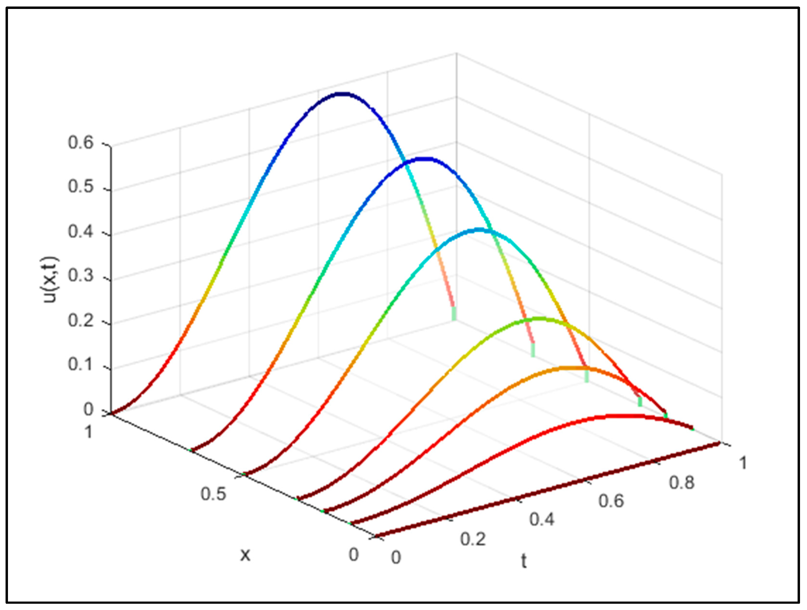
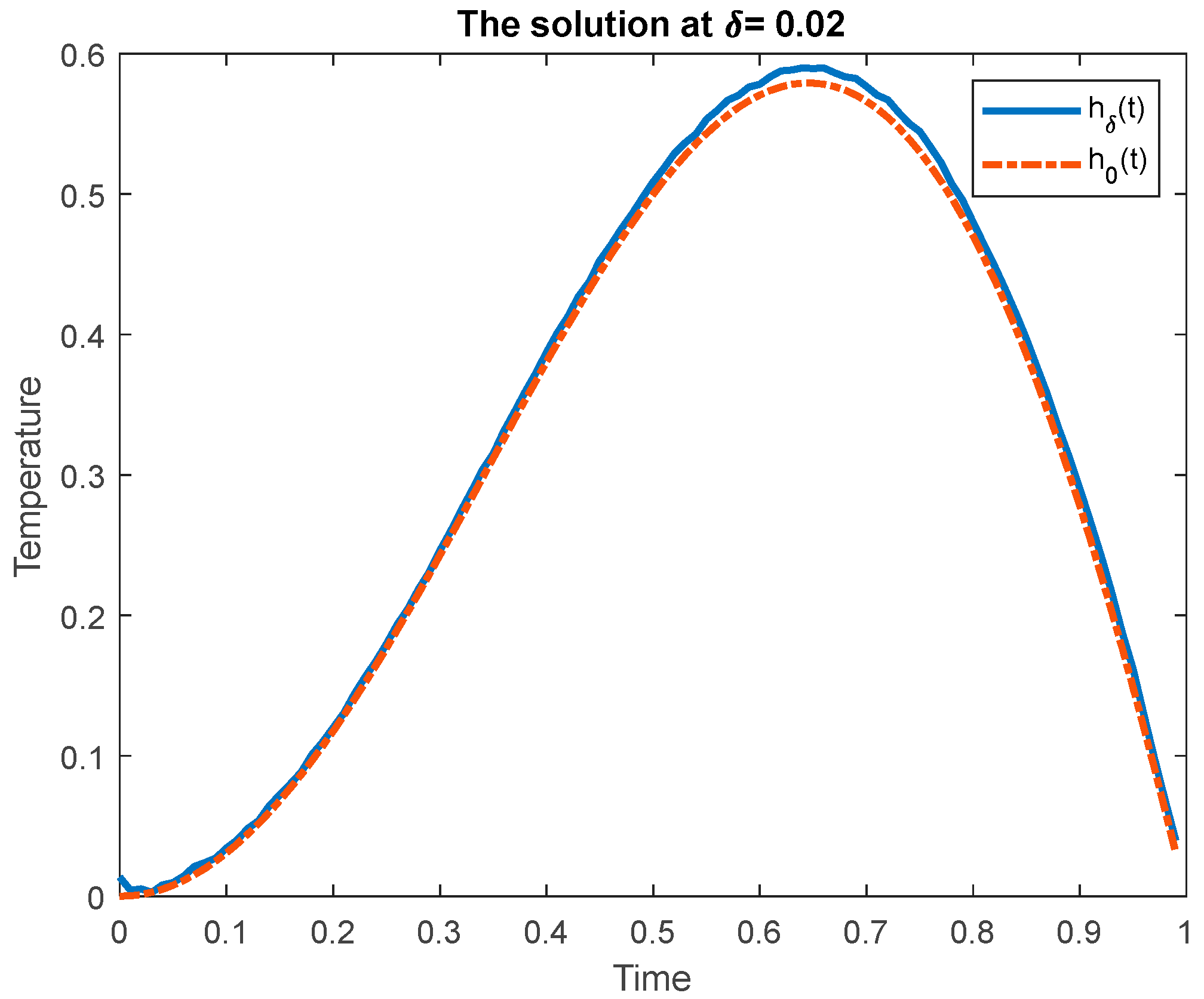
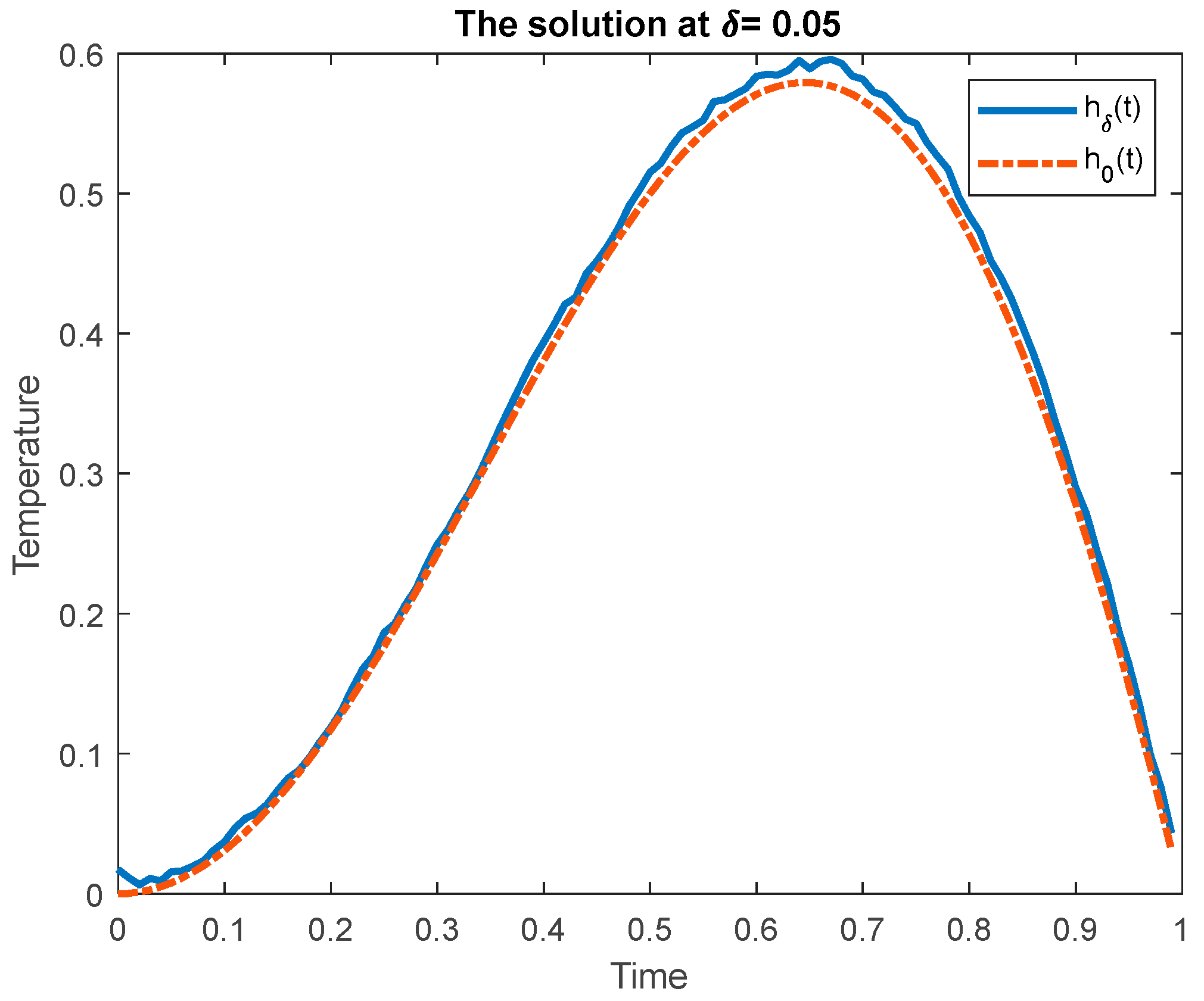
Let $\overline{H}=L_2\left(-\infty ;+\infty \right)+i{L}_2\left(-\infty ;+\infty \right)$ be the interval on the area of complex numbers, and the set of correction class $M_r\subset \overline{H}$ demarcated by the following

$$M_r=\left\{h(t):h(t)\in \overline{H},{\displaystyle \underset{0}{\overset{\infty }{\int }}{\left|h(t)\right|}^{2}dt+{\displaystyle \underset{}{\overset{}{\int }}{\left|h^{\prime }(t)\right|}^{2}dt\le r^2}}\right\},$$

(42)

$r$ known positive number.

In order to resolve the problem (1)–(5) and (18)–(21), we present $F$, as the operator which is mapping from $\overline{H}$ to $\overline{H}$ and we named as the operator via the Fourier transform

$$\widehat{h}(\tau )=F\left[h(t)\right]=\frac{1}{\sqrt{2\pi }}{\displaystyle \underset{0}{\overset{+\infty }{\int }}h(t)e^{-i\tau t}dt,\tau \in ℝ,h(t)\in \overline{H}\cap {\overline{L}}_1\left(-\infty ,\infty \right)}.$$

(43)

There ${\overline{L}}_1\left(-\infty ,\infty \right)$—interval on the of complex numbers set.

Denote by $\overline{F}$ operator continuation $F$ in $\overline{H}$. Following from Plancherel’s theorem, the operator $\overline{F}$ has isometric mapping $\overline{H}$ into $\overline{H}$.

Let $\widehat{h}(\tau )\in \overline{H}$. Then, we have

$${\overline{F}}^{-1}\left[\widehat{h}(\tau )\right]=\frac{1}{\sqrt{2\pi }}\underset{N\to \infty }{\lim }{\displaystyle \underset{-N}{\overset{+N}{\int }}\widehat{h}(\tau )}{e}^{it\tau }d\tau ,-\infty <t<+\infty ,$$

(44)

where the way to the limit has the sense of the convergence of root-mean-square.

Using transform $F$, (1)–(5) and (18)–(21) come down to the following problem

$$\frac{{\partial }^2\widehat{u}(x,\tau )}{\partial x^2}=i\tau \widehat{u}(x,\tau ),x\in (0,1),-\infty <\tau <+\infty ,$$

(45)

$$\widehat{u}(0,\tau )=0,\widehat{u}(x_0,\tau )=\widehat{g}(\tau ),-\infty <\tau <+\infty ,$$

(46)

where $\widehat{u}(x,\tau )=F\left[u(x,t)\right],\widehat{g}(\tau )=F\left[g(t)\right].$

Solutions (45) and (46) are of the form

$$\widehat{u}(x,\tau )=D_1(\tau )e^{{\mu }_0\sqrt{\tau }x}+D_2(\tau )e^{-{\mu }_0\sqrt{\tau }x},\tau >0,$$

(47)

where ${\mu }_0=\frac{1}{\sqrt{2}}(1+i),$ $D_1(\tau )$ and $D_2(\tau )$ are functions that satisfy (40) and (46).

With $\widehat{u}(1,\tau )=\widehat{h}(\tau )$ we obtain

$$\widehat{h}(\tau )=\left\{\begin{array}{l}\frac{\mathrm{sh}{\mu }_0\sqrt{\tau }}{\mathrm{sh}{\mu }_0\sqrt{\tau }{x}_0}\widehat{g}(\tau ),\tau >0,\\ 0,\hspace{1em}\hspace{1em}\hspace{1em}\hspace{1em}\tau \le 0,\end{array}\right.$$

(48)

Therefore, the problem (45) and (46) reduces to the equation

$$A\widehat{h}(\tau )=\widehat{g}(\tau ),0<\tau <\infty .$$

(49)

Let ${\widehat{g}}_0(\tau )=F\left[g_0(t)\right],{\widehat{g}}_{\delta }(\tau )=F\left[g_{\delta }(t)\right]$ and, from the Formula (41), it follows that

$${‖{\widehat{g}}_{\delta }(\tau )-{\widehat{g}}_0(\tau )‖}_{\overline{H}}\le \sqrt{2}\delta .$$

(50)

Let ${\widehat{M}}_r$ denote a set of $\overline{H}$ such that ${\widehat{M}}_r\supset F\left[M_r\right]$ and

$${\widehat{M}}_r=\left\{\widehat{h}(\tau ):\widehat{h}(\tau )\in \overline{H},{\displaystyle \underset{0}{\overset{\infty }{\int }}\left(1+{\tau }^2\right)\left|\widehat{h}(\tau )\right|d\tau \le 2r^2}\right\}.$$

(51)

Since $h_0(t)\in M_r$, then ${\widehat{h}}_0(\tau )\in {\widehat{M}}_r$.

In order to find the approximation solution for (49)–(51) we use the regularizing family of operators $\left\{R_{\alpha }\right\}$, which are defined by

$${\widehat{h}}_{\delta }^{\alpha }(\tau )=R_{\alpha }\widehat{g}(\tau )=\left\{\begin{array}{l}\frac{\mathrm{sh}{\mu }_0\sqrt{\tau }}{\mathrm{sh}{\mu }_0\sqrt{\tau }{x}_0}{\widehat{g}}_{\delta }(\tau ),0\le \tau \le \alpha ,\\ 0,\hspace{1em}\hspace{1em}\hspace{1em}\hspace{1em}\hspace{1em}\tau >\alpha ,\end{array}\right.$$

(52)

For selecting a regularization parameter $\widehat{\alpha }=\widehat{\alpha }({\widehat{g}}_{\delta },\delta )$ in Equation (52) from the initial data $({\widehat{g}}_{\delta },\delta )$, use the equation ${‖A{\widehat{h}}_{\delta }^{\alpha }(\tau )-{\widehat{g}}_{\delta }(\tau )‖}^2=16{\delta }^2$.

Let us describe an estimated solution for (49) by the formulation of ${\widehat{h}}_{\delta }(\tau )={\widehat{h}}_{\delta }^{\widehat{\alpha }(g_{\delta },\delta )}(\tau )$.

This follows from the theorem formulated in the article [25] [c. 284], that

$$‖{\widehat{h}}_{\delta }(\tau )-{\widehat{h}}_0(\tau )‖\le 7\omega (\delta ,r),$$

(53)

where $\omega (\delta ,r)=\left\{‖\widehat{h}(\tau )‖:\widehat{h}(\tau )\in {\widehat{M}}_r,‖A\widehat{h}(\tau )‖\le \delta \right\}.$

Let us describe $\left\{R_{\widehat{\alpha }({\widehat{g}}_{\delta },\delta )}:0<\delta \le {\delta }_0\right\}$ as the operator for use in the regularization method in order to obtain the approximate solution for the problem. (49) in ${\widehat{M}}_r$. Now, let us introduce $\delta \in \left(0,{\delta }_0\right]$ as the quantitative characteristic of the accuracy of this method on the set ${\widehat{M}}_r$.

$${\mathsf{\Delta }}_{\delta }\left[R_{\widehat{\alpha }({\widehat{f}}_{\delta },\delta )}\right]=\underset{{\widehat{f}}_0,{\widehat{f}}_{\delta }}{\sup }\left\{‖R_{\widehat{\alpha }({\widehat{g}}_{\delta },\delta )}{\widehat{g}}_{\delta }(\tau )-{\widehat{h}}_0(\tau )‖:{\widehat{h}}_0(\tau )\in {\widehat{M}}_r,{\widehat{g}}_{\delta }(\tau )\in H,‖{\widehat{g}}_{\delta }(\tau )-A{\widehat{h}}_0(\tau )‖\le \delta \right\}.$$

From the theorem proved in [23], it follows that the following estimate holds

$${\mathsf{\Delta }}_{\delta }\left[R_{\widehat{\alpha }({\widehat{g}}_{\delta },\delta )}\right]\ge \omega (\delta ,r).$$

(54)

Let

$${\mathsf{\Phi }}^2(\alpha )=\sup \left\{{\displaystyle \underset{\alpha }{\overset{\infty }{\int }}{\left|{\widehat{h}}_0(\tau )\right|}^{2}d\tau :{\widehat{h}}_0(\tau )\in {\widehat{M}}_r}\right\}.$$

(55)

From (51) and (55), we obtain ${\mathsf{\Phi }}^2(\alpha )=\frac{2r^2}{1+{\alpha }^2}$ for ${\widehat{h}}_0(\tau )\in {\widehat{M}}_r$.

Lemma 6.

Let${\alpha }_0=\frac{1}{2x_0^2}{\ln }^{2}2$. Then, for$\alpha \ge {\alpha }_0$the ratio is true

$$\frac{1}{4}{e}^{(1-x_0)\sqrt{\frac{\alpha }{2}}}\le ‖R_{\alpha }‖\le 4e^{(1-x_0)\sqrt{\frac{\alpha }{2}}}.$$

Lemma 6 tracks from the explanation of the operator norm. According to [26], lemma 2, to compute the modulus of continuity, $\omega (\delta ,r)$ we need to solve

$$r\alpha G(\alpha )=\delta .$$

(56)

Solving $\overline{\alpha }(\delta )$ is replaced into the function $G(\alpha )$ parameter determined by

$$\tilde{G}(\beta )=\frac{1}{\sqrt{1+{\beta }^2}},\alpha =e^{\left(x_0-1\right)\sqrt{\frac{\beta }{2}}}.$$

(57)

From (56) and (57), it follows that

$$\omega (\delta ,r)=rG(\overline{\alpha }(\delta )).$$

(58)

Therefore, from (53), (57) and (58), we obtain the estimate

$$‖{\widehat{h}}_{\delta }(\tau )-{\widehat{h}}_0(\tau )‖\le 7rG(\overline{\alpha }(\delta )).$$

(59)

In order to simplify the assessment (59), consider the equations

$$e^{(x_0-1)\sqrt{\frac{\alpha }{2}}}=\frac{r}{\delta },e^{2(x_0-1)\sqrt{\frac{\alpha }{2}}}=\frac{r}{\delta }.$$

(60)

Let ${\overline{\alpha }}_1(\delta )$ and ${\overline{\alpha }}_2(\delta )$, respectively, be solutions of the Equation (60).

Then, from (56), (60), we find that, for sufficiently small $\delta$, defined ${\overline{\alpha }}_2(\delta )$, the following relations are valid

$${\overline{\alpha }}_2(\delta )\le \overline{\alpha }(\delta )\le {\overline{\alpha }}_1(\delta ),$$

where ${\overline{\alpha }}_1(\delta )=\frac{2}{{\left(x_0-1\right)}^2}{\ln }^2\frac{r}{\delta }$, ${\overline{\alpha }}_2(\delta )=\frac{2}{2{\left(x_0-1\right)}^2}{\ln }^2\frac{r}{\delta }$ and, from the resulting inequality, we have

$$\overline{\alpha }(\delta )\sim {\ln }^2\delta at\delta \to 0.$$

From the theorem proved in [26], it follows that

$$G({\overline{\alpha }}_2(\delta ))\le G(\overline{\alpha }(\delta ))\le G({\overline{\alpha }}_1(\delta )),$$

(61)

where

$$G({\overline{\alpha }}_1(\delta ))=\frac{4}{\sqrt{1+\frac{4}{{\left(x_0-1\right)}^4}{\ln }^4\delta }},G({\overline{\alpha }}_2(\delta ))=\frac{1}{4\sqrt{1+\frac{1}{{\left(x_0-1\right)}^4}{\ln }^4\delta }},$$

(62)

from (54) we find that this is an exact ordinal estimate,

$$\sup \left\{\begin{array}{l}‖{\widehat{h}}_{\delta }^{\overline{\alpha }(\delta )}(\sigma )-{\widehat{h}}_0(\sigma )‖:{\widehat{h}}_0(\sigma )\in {\widehat{M}}_r,\\ ‖{\widehat{g}}_{\delta }(\sigma )-{\widehat{g}}_0(\sigma )‖\le \delta \end{array}\right\}\ge \frac{r}{4\sqrt{1+\frac{1}{4{(x_0-1)}^4}{\ln }^4\frac{r}{\delta }}}.$$

(63)

From lemma 5, (53) and (63) we obtain

Theorem 2.

For method$\left\{R_{\widehat{\alpha }({\widehat{g}}_{\delta },\delta )}:0<\delta \le {\delta }_0\right\}$we have an exact estimate of the order error

$$\frac{r}{4\sqrt{1+\frac{1}{4{(x_0-1)}^4}{\ln }^4\delta }}\le {\mathsf{\Delta }}_{\delta }\left[R_{\widehat{\alpha }(f_{\delta },\delta )}\right]\le \frac{74r}{\sqrt{1+\frac{1}{4{(x_0-1)}^4}{\ln }^4\delta }}.$$

(64)

Applying к ${\widehat{q}}_{\delta }(\tau )$ transformation

$$h_{\delta }(t)=\left\{\begin{array}{l}\mathrm{Re}\left[{\overline{F}}^{-1}\left[{\widehat{h}}_{\delta }(\tau )\right]\right],t\ge 0,\\ 0,\hspace{1em}\hspace{1em}\hspace{1em}\hspace{1em}\hspace{1em}t<0,\end{array}\right.$$

(65)

where ${\overline{F}}^{-1}$ is the inverse Fourier transform operator, we obtain an estimated solution for the problem (1)–(5) and (18)–(21).

Thus, for an approximate solution $h_{\delta }(t)$ for problem (1)–(5) and (18)–(21), we have a precise error estimation by

$$‖h_{\delta }(t)-h_0(t)‖\le \frac{28r}{\sqrt{1+\frac{4}{{\left(x_0-1\right)}^4}{\ln }^4\delta }}.$$

(66)

6. Case Study

Consider the function $h_0(t)=\left\{\begin{array}{l}t\sin (\pi t),t\in \left(0,T\right],\\ 0,\hspace{1em}\hspace{1em}t\in \left(T,\infty \right),\end{array}\right.$ suppose $T=1,x_0=0.5\mathrm{and}N=100$.

From the solution of the direct problem (1)–(5) and (18)–(21), we find $u_0(x_0,t)=g_0(t).$ We set a partition of the time interval $\left[0,T\right]$ with the number of nodes $N$ such that

$$0=t_0<t_1<t_2<\dots <t_n=T,t_k=\frac{k}{N},k=\overline{0,N}.$$

This simulates the one-dimensional nature of the heat equation using the Fast Fourier Transform, FFT, as shown in Figure 1. In this example, the PDE system is linear, and it is possible to advance the system directly in the frequency domain.

From Figure 1 we find $g_{\delta }(t)$, introducing an error level ${\delta }_1=0.05$ and ${\delta }_2=0.02$ in $g_0(t)$ by the following

$$g_{\delta }^k=g_0(t_k)+\frac{{\delta }_j}{\sqrt{T}}.\gamma ,j=1,2,$$

where the error level can compute by

$$‖g_{\delta }-g_0‖.$$

Figure 2 and Figure 3 show the visualization of the function as a solution for the inverse problem with $\delta =0.02$ and $\delta =0.05$, respectively. The real solution is shown by a dotted line and the approximate solution is shown by a line.

7. Conclusions

In this work, the inverse BVP of a thermal conductivity equation in two different intervals of time was solved. The heating process for an object was definitively separated into two intervals: the first one, by the heating of the boundary part or place in domain, and the second one, by the free cooling of the object. It has been verified that the boundary function or condition fits the space $H^1\left[0,\infty \right]$. This means we can use the projection regularization method for solving this problem by using the Fourier transform for time. The error estimate was obtained for the solution.

References

1. Tikhonov, A.N. On the Regularization of Ill-Posed Problems. Proc. USSR Acad. Sci. 1963, 153, 49–52. [Google Scholar]
2. Lavrent’ev, M.M. On Certain Ill-Posed Problems of Mathematical Physics; Sobolev Division of the USSR Academy Science: Novosibirsk, Russia, 1962. [Google Scholar]
3. Ivanov, V.K.; Vasin, V.V.; Tanana, V.P. Theory of Linear Ill-Posed Problem and Application; Nauok: Moscow, Russia, 1978. [Google Scholar]
4. John, F. Numerical solution of the equation of heat conduction for preceding times. Ann. di Mat. pura ed Appl. 1955, 40, 129–142. [Google Scholar] [CrossRef]
5. Cheniguel, A. Numerical method for the heat equation with Dirichlet and Neumann conditions. Proc. Int. MultiConference Eng. Comput. Sci. 2014, 1, 12–14. [Google Scholar]
6. Alifanov, O.M.; Artioukhine, E.A.; Rumyantsev, S.V. Extreme Methods for Solving Ill-Posed Problems with Applications to Inverse Heat Transfer Problems; Begell House: New York, NY, USA, 1995; ISBN 156700038X. [Google Scholar]
7. Bergman, T.L.; Incropera, F.P.; DeWitt, D.P.; Lavine, A.S. Fundamentals of Heat and Mass Transfer; John Wiley & Sons: Hoboken, NJ, USA, 2011; ISBN 0470501979. [Google Scholar]
8. Dmitriev, V.I.; Stolyarov, L.V. Numerical method for the inverse boundary-value problem of the heat equation. Comput. Math. Model. 2017, 28, 141–147. [Google Scholar] [CrossRef]
9. Sidikova, A.I. Approximate Solution of Inverse Boundary Value Problem for Heat Conduction Equation. In Proceedings of the 2018 International Russian Automation Conference (RusAutoCon), Sochi, Russia, 9–16 September 2018; pp. 1–7. [Google Scholar]
10. Sidikova, A.I. A Study of an Inverse Boundary Value Problem for the Heat Conduction Equation. Numer. Anal. Appl. 2019, 12, 70–86. [Google Scholar] [CrossRef]
11. Tanana, V.P.; Markov, B.A. The control problem for the heat equation in the case of a composite material. J. Phys. Conf. Ser. 2021, 1715, 12049. [Google Scholar] [CrossRef]
12. Makhtoumi, M. Numerical solutions of heat diffusion equation over one dimensional rod region. arXiv 2018, arXiv:1807.09588. [Google Scholar]
13. Sidikova, A.I.; Al-Mahdawi, H.K. The solution of inverse boundary problem for the heat exchange for the hollow cylinder. AIP Conf. Proc. 2022, 2398, 60050. [Google Scholar]
14. Al-Mahdawi, H.K.I.; Abotaleb, M.; Alkattan, H.; Tareq, A.-M.Z.; Badr, A.; Kadi, A. Multigrid Method for Solving Inverse Problems for Heat Equation. Mathematics 2022, 10, 2802. [Google Scholar] [CrossRef]
15. Al-Mahdawi, H.K.; Sidikova, A.I. Iterated Lavrent’ev regularization with the finite-dimensional approximation for inverse problem. AIP Conf. Proc. 2022, 2398, 60080. [Google Scholar]
16. Al-Mahdawi, H.K.; Sidikova, A.I.; Alkattan, H.; Abotaleb, M.; Kadi, A.; El-kenawy, E.-S.M. Parallel Multigrid Method for Solving Inverse Problems. MethodsX 2022, 9, 101887. [Google Scholar] [CrossRef] [PubMed]
17. Al-Mahdawi, H.K.I.; Alkattan, H.; Abotaleb, M.; Kadi, A.; El-kenawy, E.-S.M. Updating the Landweber Iteration Method for Solving Inverse Problems. Mathematics 2022, 10, 2798. [Google Scholar] [CrossRef]
18. Glasko, V.B.; Kulik, N.I.; Shklyarov, I.N.; Tikhonov, A.N. An inverse problem of heat conductivity. Zhurnal Vychislitel’noi Mat. I Mat. Fiz. 1979, 19, 768–774. [Google Scholar]
19. Belonosov, A.S.; Shishlenin, M.A. Continuation problem for the parabolic equation with the data on the part of the boundary. Siber. Electron. Math. Rep. 2014, 11, 22–34. [Google Scholar]
20. Kabanikhin, S.I.; Hasanov, A.; Penenko, A.V. A gradient descent method for solving an inverse coefficient heat conduction problem. Numer. Anal. Appl. 2008, 1, 34–45. [Google Scholar] [CrossRef]
21. Yagola, A.G.; Stepanova, I.E.; Van, Y.; Titarenko, V.N. Obratnye zadachi i metody ikh resheniya. Prilozheniya k geofizike. In Inverse Problems and Methods for their Solution: Applications to Geophysics; BKL Publishers: Moscow, Russia, 2014. [Google Scholar]
22. Kabanikhin, S.I.; Krivorot’ko, O.I.; Shishlenin, M.A. A numerical method for solving an inverse thermoacoustic problem. Numer. Anal. Appl. 2013, 6, 34–39. [Google Scholar] [CrossRef]
23. Tanana, V.P. On the order-optimality of the projection regularization method in solving inverse problems. Sib. Zhurnal Ind. Mat. 2004, 7, 117–132. [Google Scholar]
24. Farlow, S.J. Partial Differential Equations for Scientists and Engineers; Courier Corporation: North Chelmsford, MA, USA, 1993; ISBN 048667620X. [Google Scholar]
25. Tanana, V.P.; Bredikhina, A.B.; Kamaltdinova, T.S. On an error estimate for an approximate solution for an inverse problem in the class of piecewise smooth functions. Tr. Inst. Mat. I Mekhaniki UrO RAN 2012, 18, 281–288. [Google Scholar]
26. Tanana, V.P.; Rudakova, T.N. The optimum of the M. M. Lavrent’ev method. J. Inverse Ill-Posed Probl. 2011, 18, 935–944. [Google Scholar] [CrossRef]
Figure 1. Evolution of the direct heat Equations (45) and (46).
Algorithms 16 00033 g001
Figure 2. Visualization of the answer with δ = 0.02 .
Algorithms 16 00033 g002
Figure 3. Visualization of the answer with δ = 0.05 .
Algorithms 16 00033 g003
Disclaimer/Publisher’s Note: The statements, opinions and data contained in all publications are solely those of the individual author(s) and contributor(s) and not of MDPI and/or the editor(s). MDPI and/or the editor(s) disclaim responsibility for any injury to people or property resulting from any ideas, methods, instructions or products referred to in the content.