

Training Performance Indications for Amateur Athletes Based on Nutrition and Activity Lifelogs

 , ,
, ,  ,
,  , ,
, ,  , , and
Abstract
1. Introduction
- Find different optimal subsets of data types from multimodal lifelog datasets that can help to reduce the computational complexity of the system;
- Discover daily nutrition and activity patterns that significantly impact exercise outcomes including endurance, stamina, and weight loss; and
- Predict exercise outcomes based on daily nutrition and activities, both for a group and an individual.
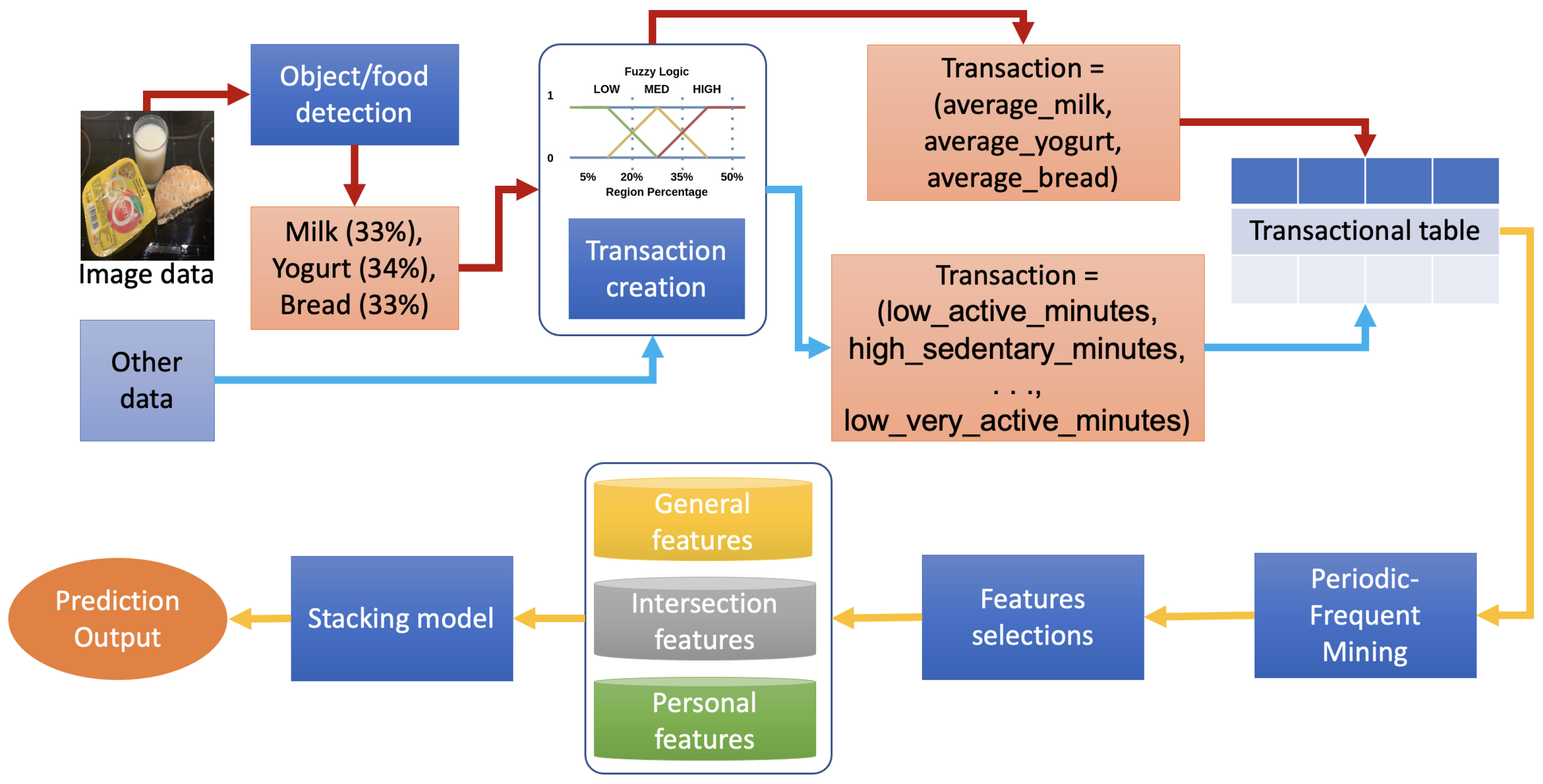
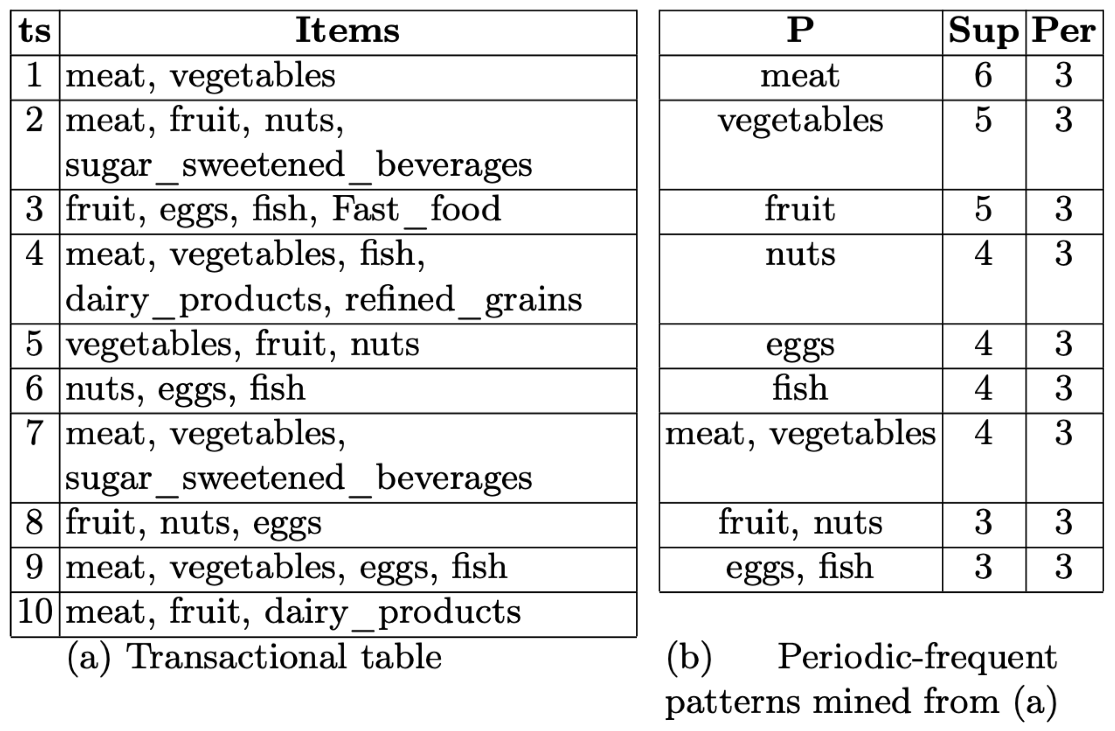
- We apply the periodic-frequent pattern mining technique [13] to discover subsets of factors that appear with a high periodic-frequent score throughout the dataset. We convert nutrition and physical activity data into a transactional table by converting continuous data into discrete data using fuzzy logic. We hypothesize that these subsets can characterize a particular group of people who share the same common points that do not appear in other groups.
- We estimate the portion of healthy and unhealthy foods from food images and treat them as numeric data. The data can enrich the nutrition factor besides food-logs reported by people. Estimating a portion of healthy food could overcome the challenge of precisely calculating calories from food images since object detection and semantic segmentation algorithms currently work better than image-to-calories approaches.
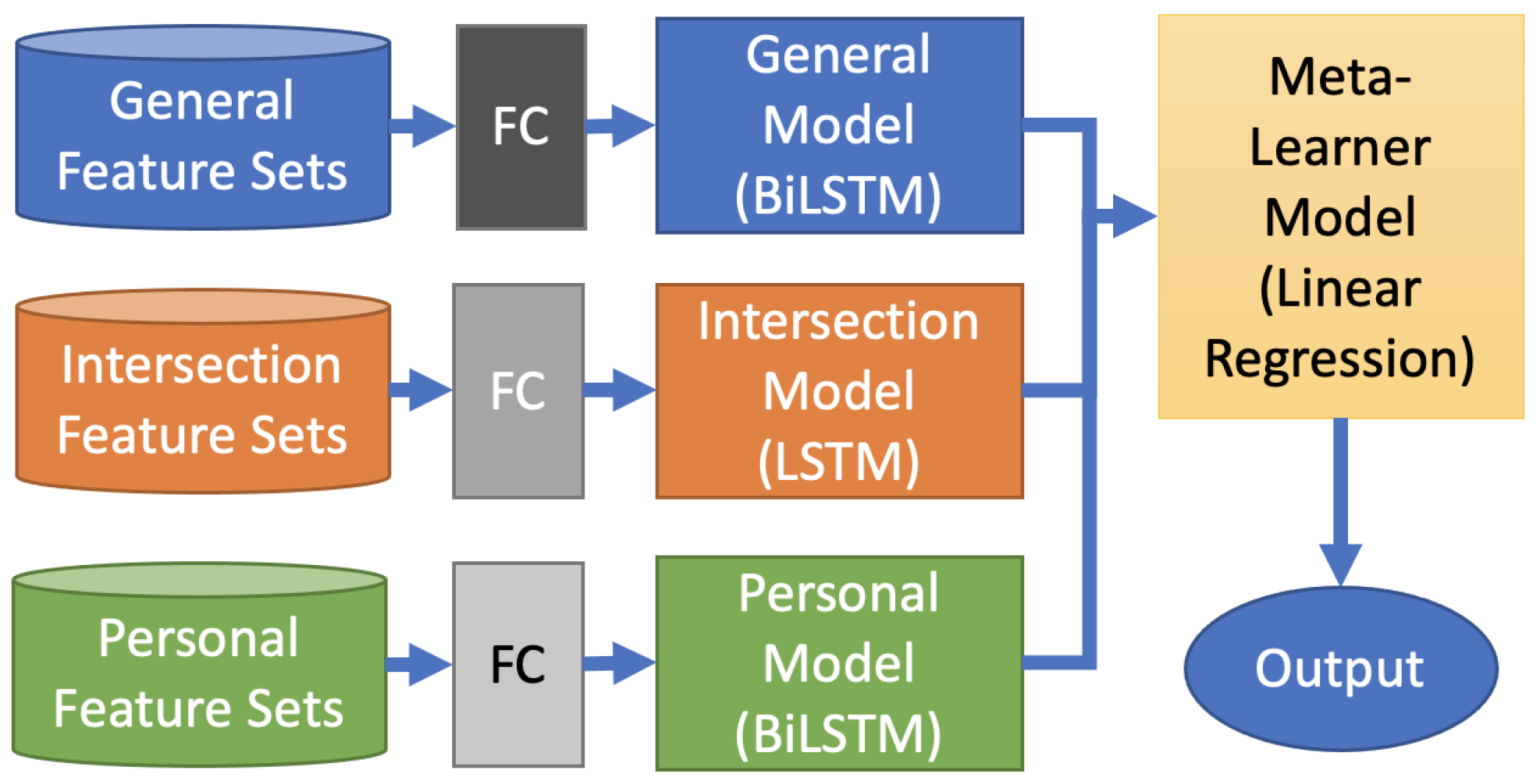
- We create a stacking model to forecast people’s weight and running speed changes based on their daily meals and workout habits. The model can adapt to different general and individual cases that suit understanding training performance throughout the nutrition and physical activities of a large-scale people group.
2. Methodology
2.1. The PMData Dataset
2.2. Periodic-Frequent Pattern Mining
2.3. Data Pre-Processing: Fuzzy Logic and Transactions
2.4. Feature Selection
- People share common characteristics with their group and have personal characteristics that make them unique from a group.
- With the same exercise and nutrition plan, finding two people with the same outcome is problematic.
- People who prefer a self-training plan tend not to follow the plan strictly due to both subjective (e.g., tired, not in the mood) and objective reasons (e.g., busy working, unexpected meeting)
2.4.1. Personal Features
2.4.2. Intersection Features
2.4.3. General Features
2.5. The Data-Driven Stacking-Based Model
3. Experimental Results
3.1. Data Grouping
3.2. Evaluations
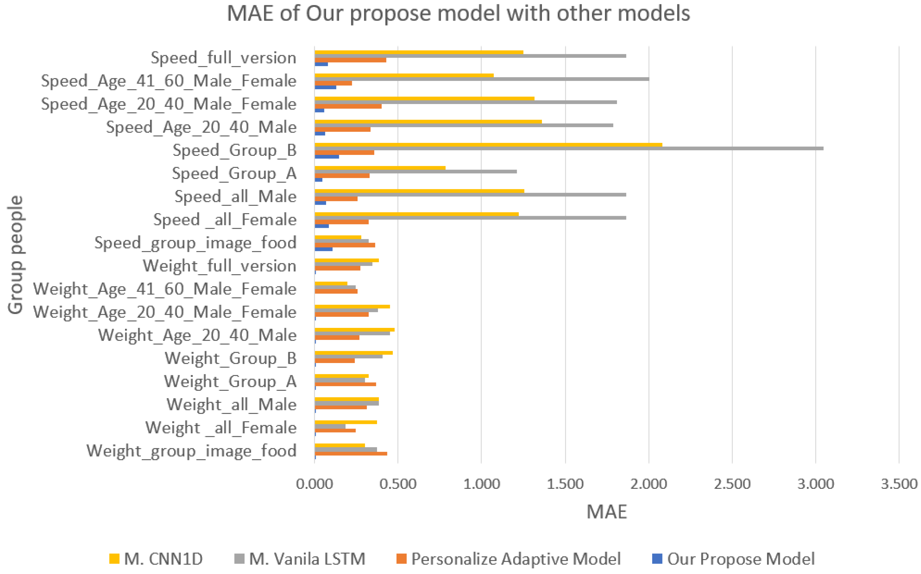
3.3. Comparisons
4. Conclusions and Future Works
Author Contributions
Funding
Data Availability Statement
Acknowledgments
Conflicts of Interest
References
- Rothschild, J.A.; Kilding, A.E.; Plews, D.J. Pre-exercise nutrition habits and beliefs of endurance athletes vary by sex, competitive level, and diet. J. Am. Coll. Nutr. 2021, 40, 517–528. [Google Scholar] [CrossRef] [PubMed]
- Thompson, W.R. Worldwide survey of fitness trends for 2020. ACSMs Health Fit. J. 2019, 23, 10–18. [Google Scholar] [CrossRef]
- Singh, V.N. A Current Perspective on Nutrition and Exercise. J. Nutr. 1992, 122, 760–765. [Google Scholar] [CrossRef] [PubMed]
- Sun, W. Sports Performance Prediction Based on Chaos Theory and Machine Learning. Wirel. Commun. Mob. Comput. 2022, 2022, 3916383. [Google Scholar] [CrossRef]
- Iyer, S.R.; Sharda, R. Prediction of athletes performance using neural networks: An application in cricket team selection. Expert Syst. Appl. 2009, 36, 5510–5522. [Google Scholar] [CrossRef]
- Ragab, N. Soccer Athlete Performance Prediction Using Time Series Analysis. Master’s Thesis, OsloMet-Storbyuniversitetet, Oslo, Norway, April 2022. [Google Scholar]
- Zhou, L.; Gurrin, C. A survey on life logging data capturing. In Proceedings of the SenseCam Symposium 2012, Oxford, UK, 3–4 April 2012. [Google Scholar]
- Gurrin, C.; Zhou, L.; Healy, G.; Jónsson, B.Þ.; Dang-Nguyen, D.; Lokoč, J.; Tran, M.; Hürst, W.; Rossetto, L.; Schöffmann, K. Introduction to the Fifth Annual Lifelog Search Challenge. In Proceedings of the 2022 International Conference on Multimedia Retrieval (LSC’22), Newark, NJ, USA, 27–30 June 2022. [Google Scholar]
- NII. NII Testbeds and Community for Information Access Research. Available online: https://research.nii.ac.jp/ntcir/index-en.html (accessed on 18 December 2022).
- Ninh, V.-T.; Le, T.-K.; Zhou, L.; Piras, L.; Riegler, M.; Halvorsen, P.L.; Tran, M.-T.; Lux, M.; Gurrin, C.; Dang-Nguyen, D.-T. Overview of ImageCLEF Lifelog 2020: Lifelog Moment Retrieval and Sport Performance Lifelog. In Proceedings of the CLEF2020 Working Notes, Ser. CEUR Workshop Proceedings, Thessaloniki, Greece, 22–25 September 2020; Available online: http://ceur-ws.org (accessed on 18 December 2022).
- Chung, S.; Jeong, C.Y.; Lim, J.M.; Lim, J.; Noh, K.J.; Kim, G.; Jeong, H. Real-world multimodal lifelog dataset for human behavior study. ETRI J. 2021, 44, 426–437. [Google Scholar] [CrossRef]
- Thambawita, V.; Hicks, S.A.; Borgli, H.; Stensland, H.K.; Jha, D.; Svensen, M.K.; Pettersen, S.A.; Johansen, D.; Johansen, H.D.; Pettersen, S.D.; et al. PMData: A sports logging dataset. In Proceedings of the 11th ACM Multimedia Systems Conference (MMSys ’20), Istanbul, Turkey, 8–11 June 2020; Association for Computing Machinery: New York, NY, USA, 2020; pp. 231–236. [Google Scholar]
- Kiran, R.U.; Kitsuregawa, M.; Reddy, P.K. Efficient discovery of periodic-frequent patterns in very large databases. J. Syst. Softw. 2016, 112, 110–121. [Google Scholar] [CrossRef]
- Chatterjee, A.; Prinz, A.; Riegler, M. Prediction Modeling in Activity eCoaching for Tailored Recommendation Generation: A Conceptualization. In Proceedings of the 2022 IEEE International Symposium on Med-ical Measurements and Applications (MeMeA), Messina, Italy, 22–24 June 2022; pp. 1–6, ISBN 978-1-6654-8299-8. [Google Scholar] [CrossRef]
- Karami, Z.; Hines, A.; Jahromi, H. Leveraging IoT Lifelog Data to Analyse Perfor-mance of Physical Activities. In Proceedings of the 2021 32nd Irish Signals and Systems Conference (ISSC), Athlone, Ireland, 10–11 June 2021; pp. 1–6, ISBN 978-1-6654-3429-4. [Google Scholar] [CrossRef]
- Diaz, C.; Caillaud, C.; Yacef, K. Unsupervised Early Detection of Physical Ac-tivity Behaviour Changes from Wearable Accelerometer Data. Sensors 2022, 22, 8255. [Google Scholar] [CrossRef] [PubMed]
- Kazuki, T.; Dao, M.; Zettsu, K. MM-AQI: A Novel Framework to Understand the Associations Between Urban Traffic, Visual Pollution, and Air Pollution. In Proceedings of the IEA/AIE, Kitakyushu, Japan, 19–22 July 2022; pp. 597–608. [Google Scholar]
- Haldimann, M.; Alt, A.; Blanc, A.; Blondeau, K. Iodine content of food groups. J. Food Compos. Anal. 2004, 18, 461–471. [Google Scholar]
- Schwingshackl, L.; Schwedhelm, C.; Hoffmann, G.; Knuppel, S.; Preterre, A.L.; Iqbal, K.; Bechthold, A.; Henauw, S.D.; Michels, N.; Devleesschauwer, B.; et al. Food groups and risk of colorectal cancer. IJC J. 2017, 142, 1748–1758. [Google Scholar] [CrossRef] [PubMed]
- 7ESL Homepage. 2022. Available online: https://7esl.com/fast-food-vocabulary/ (accessed on 18 December 2022).
- McKinnon, R.A.; Oladipo, T.; Ferguson, M.S.; Jones, O.E.; Maroto, M.E. Beverly Wolpert Reported Knowledge of Typical Daily Calorie Requirements: Relationship to De-mographic Characteristics in US Adults. J. Acad. Nutr. Diet. 2019, 119, 1831–1841.e6. [Google Scholar] [CrossRef] [PubMed]
- Dhal, P.; Azad, C. A comprehensive survey on feature selection in the various fields of machine learning. Appl. Intell. 2022, 52, 4543–4581. [Google Scholar] [CrossRef]
- Berk, R.A. An Introduction to Ensemble Methods for Data Analysis. SAGE J. 2006, 34. [Google Scholar] [CrossRef]
- Wang, J.; Liu, C.; Li, L.; Li, W.; Yao, L.; Li, H.; Zhang, H. A Stacking-Based Model for Non-Invasive De-tection of Coronary Heart Disease. IEEE Access 2020, 8, 37124–37133. [Google Scholar] [CrossRef]
- Van, N.T.P.; Son, D.M.; Zettsu, K. A Personalized Adaptive Algorithm for Sleep Quality Prediction using Physiological and Environmental Sensing Data. In Proceedings of the IEEE 2021 8th NAFOSTED Conference on Information and Computer Science (NICS), Hanoi, Vietnam, 21–22 December 2021. [Google Scholar]
- Mai-Nguyen, A.V.; Tran, V.L.; Dao, M.S.; Zettsu, K. Leverage the Predictive Power Score of Lifelog Data’s Attributes to Predict the Expected Athlete Performance. In Proceedings of the CLEF, Thessaloniki, Greece, 22–25 September 2020. [Google Scholar]


| Categories | File | Rate of Entries | Number of Entries |
|---|---|---|---|
| SRPE | srpe.csv | Per exercise | 783 |
| Injury | injury.csv | Per week | 225 |
| Wellness | wellness.csv | Per day | 1747 |
| Steps | steps.json | Per minute | 1,534,705 |
| Calories | calories.json | Per minute | 3,377,529 |
| Distance | distance.json | Per minute | 1,534,705 |
| Exercise | exercise.json | When it happens (100 entries per file) | 2440 |
| Heart rate | heart_rate.json | Per 5 s | 20,991,392 |
| Lightly active minutes | lightly_active_minutes.json | Per day | 2244 |
| Sedentary minutes | sedentary_minutes.json | Per day | 2396 |
| Moderately active minutes | moderately_active_minutes.json | Per day | 2396 |
| Very active minutes | very_active_minutes.json | Per day | 2396 |
| Resting heart rate | resting_heart_rate.json | Per day | 1803 |
| Sleep | sleep.json | When it happens (usually daily) | 2064 |
| Sleep score | sleep_score.csv | When it happens (usually daily) | 1836 |
| Time in heart rate zones | time_in_heart_rate_zones.json | Per day | 2178 |
| Google Forms reporting | reporting.csv | Per day | 1569 |
| Features | Low Level | Normal Level | High Level |
|---|---|---|---|
| Calories_all_day | 0–2000 | 2000–3000 | 3000–6000 |
| exercise_calories | 0–200 | 200–450 | 450–6000 |
| distance | 0–7000 | 7000–9000 | 9000–25,000 |
| exercise_distance | 0–4000 | 4000–7000 | 7000–25,000 |
| lightly_active_minutes | 0–1800 | 1800–2100 | 2100–42,000 |
| exercise_lightly_minutes | 0–1800 | 1800–2100 | 2100–42,000 |
| steps | 0–10,000 | 10,000–18,000 | 18,000–30,000 |
| exercise_steps | 0–2000 | 2000–4000 | 4000–30,000 |
| moderately_active_minutes | 0–6300 | 6300–6900 | 9000 |
| exercise_moderately_minutes | 0–6300 | 6300–6900 | 9000 |
| sedentary_minutes | 0–600 | 600–1800 | 1800–90,000 |
| exercise_sedentary_minutes | 0–600 | 600–1800 | 1800–90,000 |
| very_active_minutes | 0–15,000 | 15,000–15,600 | 15,600–120,000 |
| exercise_very_minutes | 0–15,000 | 15,000–15,600 | 15,600–120,000 |
| exercise_averageHeartRate | 0–95 | 95–170 | 170–2000 |
| exercise_speed | 0–7 | 7–9 | 9–15 |
| exercise_duration | 0–1500 | 1500–2100 | 2100–9000 |
| time_per_kilometer | 0–1500 | 1500–2100 | 2100–9000 |
| exercise_elevationGain | 0–15 | 15–100 | 100–300 |
| exercise_heartRateZones_FatBurn_minutes | 0–3600 | 3600–5100 | 5100–120,000 |
| exercise_heartRateZones_Peak_minutes | 0–11,220 | 11,220–12,000 | 12,000–30,000 |
| exercise_heartRateZones_Cardio_minutes | 0–6180 | 6180–7500 | 7500–30,000 |
| Name of Group | Person in Group |
|---|---|
| Weight_Group_Image_food | p01, p03, p05 |
| Weight_all_Female | p04, p10, p11 |
| Weight_all_Male | p01, p02, p03, p05, p06, p07, p08, p09, p12, p13, p14, p16 |
| Weight_Group_A | p01, p02, p03, p04, p05, p11, p12, p13, p14 |
| Weight_Group_B | p06, p07, p08, p09, p10, p16 |
| Weight_Group_Age_20_40_Male p16 | p03, p05, p06, p07, p08, p09, p12, p13, p16 |
| Weight_Group_Age_20_40_Male_and_Female | p03, p04, p05, p07, p08, p09, p10, p11, p12, p13, p16 |
| Weight_Group_Age_41_60Male_and_Female | p01, p02, p06, p14 |
| Weight_all_people | p01, p02, p03, p04, p05, p06, p07, p08, p09, p10, p11, p12, p13, p14, p16 |
| Speed_Group_Image_food | p01, p03, p05 |
| Speed_all_Female | p04, p10, p11 |
| Speed _all_Male | p01, p02, p03, p05, p06, p07, p08, p09, p12, p13, p14 |
| Speed _Group_A | p01, p02, p03, p04, p05, p11, p12, p13, p14 |
| Speed _Group_B | p06, p07, p08, p09, p10 |
| Speed _Group_Age_20_40_Male | p03, p05, p06, p07, p08, p09, p12, p13 |
| Speed _Group_Age_20_40_Male_and_Female | p03, p04, p05, p07, p08, p09, p10, p11, p12, p13 |
| Speed _Group_Age_41_60Male_and_Female | p01, p02, p06, p14 |
| Speed_all_people | p01, p02, p03, p04, p05, p06, p07, p08, p09, p10, p11, p12, p13, p14 |
| Name of Group | General Model | Intersection Model | Personal Model | Stacking Model | ||||
|---|---|---|---|---|---|---|---|---|
| MAE | MSE | MAE | MSE | MAE | MSE | MAE | MSE | |
| Weight_group_image_food | 0.416 | 0.256 | 0.408 | 0.235 | 0.458 | 0.367 | 0.006 | 0.002 |
| Weight _all_Female | 0.378 | 0.198 | 0.366 | 0.181 | 0.221 | 0.072 | 0.009 | 0.005 |
| Weight_all_Male | 0.322 | 0.138 | 0.376 | 0.167 | 0.391 | 0.237 | 0.003 | 0.001 |
| Weight_Group_A | 0.459 | 0.248 | 0.480 | 0.236 | 0.280 | 0.150 | 0.002 | 0.001 |
| Weight_Group_B | 0.238 | 0.090 | 0.509 | 0.290 | 0.237 | 0.088 | 0.007 | 0.003 |
| Weight_Age_20_40_Male | 0.371 | 0.169 | 0.443 | 0.205 | 0.225 | 0.075 | 0.005 | 0.001 |
| Weight_Age_20_40_Male_Female | 0.372 | 0.188 | 0.428 | 0.190 | 0.265 | 0.130 | 0.006 | 0.002 |
| Weight_Age_41_60_Male_Female | 0.270 | 0.127 | 0.293 | 0.122 | 0.203 | 0.061 | 0.000 | 0.000 |
| Weight_full_version | 0.231 | 0.082 | 0.371 | 0.158 | 0.263 | 0.122 | 0.005 | 0.002 |
| Speed_group_image_food | 0.169 | 0.039 | 0.126 | 0.024 | 0.225 | 0.086 | 0.107 | 0.020 |
| Speed _all_Female | 0.182 | 0.051 | 0.102 | 0.021 | 0.331 | 0.152 | 0.086 | 0.018 |
| Speed_all_Male | 0.134 | 0.031 | 0.078 | 0.014 | 0.349 | 0.181 | 0.067 | 0.012 |
| Speed_Group_A | 0.112 | 0.023 | 0.057 | 0.011 | 0.387 | 0.182 | 0.049 | 0.009 |
| Speed_Group_B | 0.175 | 0.043 | 0.171 | 0.034 | 0.463 | 0.286 | 0.145 | 0.029 |
| Speed_Age_20_40_Male | 0.150 | 0.037 | 0.073 | 0.012 | 0.454 | 0.247 | 0.062 | 0.010 |
| Speed_Age_20_40_Male_Female | 0.111 | 0.021 | 0.069 | 0.009 | 0.421 | 0.217 | 0.058 | 0.007 |
| Speed_Age_41_60_Male_Female | 0.151 | 0.038 | 0.253 | 0.077 | 0.322 | 0.153 | 0.128 | 0.033 |
| Speed_full_version | 0.119 | 0.024 | 0.095 | 0.016 | 0.345 | 0.170 | 0.081 | 0.013 |
| Patterns | Support (%) | Periodicity (%) |
|---|---|---|
| low_moderately_active_minutes, high_sedentary_minutes, low_very_active_minutes | 0.99 | 2 |
| low_glasses_of_fluid | 0.96 | 6 |
| Yes_Breakfast, Yes_Dinner | 0.37 | 16 |
| high_Fast_food | 0.14 | 24 |
Disclaimer/Publisher’s Note: The statements, opinions and data contained in all publications are solely those of the individual author(s) and contributor(s) and not of MDPI and/or the editor(s). MDPI and/or the editor(s) disclaim responsibility for any injury to people or property resulting from any ideas, methods, instructions or products referred to in the content. |
© 2023 by the authors. Licensee MDPI, Basel, Switzerland. This article is an open access article distributed under the terms and conditions of the Creative Commons Attribution (CC BY) license (https://creativecommons.org/licenses/by/4.0/).
Share and Cite
Nguyen, P.-T.; Dao, M.-S.; Riegler, M.A.; Kiran, R.U.; Dang, T.-T.; Le, D.-D.; Nguyen-Ly, K.-C.; Pham, T.-Q.; Nguyen, V.-L. Training Performance Indications for Amateur Athletes Based on Nutrition and Activity Lifelogs. Algorithms 2023, 16, 30. https://doi.org/10.3390/a16010030
Nguyen P-T, Dao M-S, Riegler MA, Kiran RU, Dang T-T, Le D-D, Nguyen-Ly K-C, Pham T-Q, Nguyen V-L. Training Performance Indications for Amateur Athletes Based on Nutrition and Activity Lifelogs. Algorithms. 2023; 16(1):30. https://doi.org/10.3390/a16010030
Chicago/Turabian StyleNguyen, Phuc-Thinh, Minh-Son Dao, Michael A. Riegler, Rage Uday Kiran, Thai-Thinh Dang, Duy-Dong Le, Kieu-Chinh Nguyen-Ly, Thanh-Qui Pham, and Van-Luong Nguyen. 2023. "Training Performance Indications for Amateur Athletes Based on Nutrition and Activity Lifelogs" Algorithms 16, no. 1: 30. https://doi.org/10.3390/a16010030
APA StyleNguyen, P.-T., Dao, M.-S., Riegler, M. A., Kiran, R. U., Dang, T.-T., Le, D.-D., Nguyen-Ly, K.-C., Pham, T.-Q., & Nguyen, V.-L. (2023). Training Performance Indications for Amateur Athletes Based on Nutrition and Activity Lifelogs. Algorithms, 16(1), 30. https://doi.org/10.3390/a16010030