Article

Training Performance Indications for Amateur Athletes Based on Nutrition and Activity Lifelogs

1
University of Information Technology, Ho Chi Minh City 700000, Vietnam
2
Vietnam National University, Ho Chi Minh City 700000, Vietnam
3
National Institute of Information and Communications Technology, Tokyo 184-8795, Japan
4
Simula Research Laboratory, 0164 Oslo, Norway
5
Aizu University, Fukushima 965-8580, Japan
6
University of Economic Ho Chi Minh City (UEH), Ho Chi Minh City 700000, Vietnam
*
Author to whom correspondence should be addressed.
Algorithms 2023, 16(1), 30; https://doi.org/10.3390/a16010030
Submission received: 18 September 2022 / Revised: 5 December 2022 / Accepted: 19 December 2022 / Published: 4 January 2023

Abstract

:
To maintain and improve an amateur athlete’s fitness throughout training and to achieve peak performance in sports events, good nutrition and physical activity (general and training specifically) must be considered as important factors. In our context, the terminology “amateur athletes” represents those who want to practice sports to protect their health from sickness and diseases and improve their ability to join amateur athlete events (e.g., marathons). Unlike professional athletes with personal trainer support, amateur athletes mostly rely on their experience and feeling. Hence, amateur athletes need another way to be supported in monitoring and recommending more efficient execution of their activities. One of the solutions to (self-)coaching amateur athletes is collecting lifelog data (i.e., daily data captured from different sources around a person) to understand how daily nutrition and physical activities can impact their exercise outcomes. Unfortunately, not all factors of the lifelog data can contribute to understanding the mutual impact of nutrition, physical activities, and exercise frequency on improving endurance, stamina, and weight loss. Hence, there is no guarantee that analyzing all data collected from people can produce good insights towards having a good model to predict what the outcome will be. Besides, analyzing a rich and complicated dataset can consume vast resources (e.g., computational complexity, hardware, bandwidth), and this therefore does not suit deployment on IoT or personal devices. To meet this challenge, we propose a new method to (i) discover the optimal lifelog data that significantly reflect the relation between nutrition and physical activities and training performance and (ii) construct an adaptive model that can predict the performance for both large-scale and individual groups. Our suggested method produces positive results with low MAE and MSE metrics when tested on large-scale and individual datasets and also discovers exciting patterns and correlations among data factors.

1. Introduction

Everyone’s health can benefit from regular exercise and good nutrition, especially amateur athletes [1]. To determine health trends across various age groups, the research introduced in [2] pointed out that people pay a great deal of attention to which type of nutrition and physical activities they need to perform during exercising to gain better performance. In [3], the authors mention people’s interest in the correlation between nutrition, sleeping qualification, training regimen, and health. With hard training without eating or sleeping healthily, people cannot improve their performance, and their health will probably deteriorate.
Beyond this, people want to predict training performance for various objects (e.g., professional and amateur athletes, college students, older people) based on people’s daily routines, such as nutrition, sleeping, physical activities, habits, and demographic data. In [4], a model built by neural networks and chaos theory is proposed to predict the training performance of college students. The model’s accuracy is over 90%, and most of the data pertain to athletic performance measurements. In [5], a neural network model using player performance data is built to forecast the performance of cricket athletes. An LSTM model is introduced in [6] to predict soccer athletes’ performance. These studies focus on a narrow domain that rarely shares the same common points, such as professional athletes and college students. Moreover, these studies do not consider nutrition, one of the most critical factors impacting training performance.
It cannot be denied that the mentioned datasets are very helpful in supporting professional athletes to improve their training. Unfortunately, due to a lack of resources, ordinary people or amateur athletes cannot afford such datasets for their training.
Recently, lifelogs have become a new trend to monitor the daily activities of individuals by utilizing both friendly and economic IoT and wearable devices (e.g., Fitbit, camera, smartphone, ECG) and conventional diaries (e.g., self-reports, multi-choices, tags) to collect personal data reflecting all aspects of personal life [7]. Such datasets can be an excellent resource for building a personal coaching application. In recent decades, many challenges and tasks aimed at obtaining insights into lifelog data have been organized, such as LSC (Lifelog Search Challenge) [8], NTCIR (NII Testbeds and Community for Information access Research—Lifelog task) [9], and CLEF (Conference and Labs of the Evaluation Forum—ImageCLEFlifelog task) [10]. Few studies have been performed related to understanding the association between daily life activities and sports performances, such as imageCLEFlifelog—SPLL task (Sport Performance Lifelog).
In [11], the authors introduce an interesting multimodal lifelog dataset that includes individuals’ dietary habits, sports participation, and health status with the aim of studying human behavior via their daily activities. This dataset contains different factors, including food pictures, heart rates, sleep qualification, exercises, and feelings. The primary motivation of this study is to combine information on various aspects of daily activities, including exercises and nutrition, to recognize human activities and extract daily behavior patterns with the aim of discovering five representative models for understanding human behavior. Although the dataset contains some information relating to sports, the authors do not aim to analyze how nutrition and physical activities can impact sports activities.
In contrast to the mentioned methods and datasets, PMData [12] aims to collect lifelog data from ordinary people who want better health by exercising independently without personal trainers. These people could be considered amateur athletes. The motivation of the person who created this dataset is to provide a playground for those who want to create a tool that can support amateur athletes to gain better training performance by monitoring their daily routines. This motivation is expressed to the public via the ImageCLEFlifelog 2020 challenge [10], where participants are required to predict the change in running speed and weight after monitoring the amateur athlete’s dataset for a while.
Recent multimodal lifelog datasets have succeeded in collecting diverse data types that reflect daily human activities. The ambition of these datasets is to collect as much data as possible. Unfortunately, this leads to significant challenges in data analysis and prediction model construction, such as high-dimensional data, computational complexity workload, data samplings, and redundant data. Although lifelog data help to serve individual demands (e.g., searching, recommendation, activity/behavior prediction), the community needs more than that: a prediction model that can work for a large-scale group of people, and that model can easily and quickly adapt to a new coming individual who joins the community. In other words, given a set of lifelog data collected from a group of diverse people, can we build a model that can work well for both groups and individuals? Moreover, can we explain the reason or causality of the model’s output?
To meet these challenges and discover valuable and interesting insights, we propose a new method to achieve the following:
  • Find different optimal subsets of data types from multimodal lifelog datasets that can help to reduce the computational complexity of the system;
  • Discover daily nutrition and activity patterns that significantly impact exercise outcomes including endurance, stamina, and weight loss; and
  • Predict exercise outcomes based on daily nutrition and activities, both for a group and an individual.
The main contributions of our work are as follows:
  • We apply the periodic-frequent pattern mining technique [13] to discover subsets of factors that appear with a high periodic-frequent score throughout the dataset. We convert nutrition and physical activity data into a transactional table by converting continuous data into discrete data using fuzzy logic. We hypothesize that these subsets can characterize a particular group of people who share the same common points that do not appear in other groups.
  • We estimate the portion of healthy and unhealthy foods from food images and treat them as numeric data. The data can enrich the nutrition factor besides food-logs reported by people. Estimating a portion of healthy food could overcome the challenge of precisely calculating calories from food images since object detection and semantic segmentation algorithms currently work better than image-to-calories approaches.
  • We create a stacking model to forecast people’s weight and running speed changes based on their daily meals and workout habits. The model can adapt to different general and individual cases that suit understanding training performance throughout the nutrition and physical activities of a large-scale people group.
The rest of the paper is structured as follows: Section 2 introduces the data-driven approach with which we build the model. Section 3 presents the evaluation and comparison of our model together with necessary discussions. The last section concludes the paper and proposes the next research step on the same topic.

2. Methodology

This section introduces the data-driven approach with which we build our model. First, we introduce the dataset and how to discrete it into a transactional table ready for mining periodic-frequent patterns. Then, we briefly introduce the periodic-frequent pattern mining algorithm and how to utilize it to discover valuable subsets of data factors (i.e., feature selection) with which we can discriminate among people groups. Next, we present the data-driven stacking-based model running on mined subsets of data factors. Finally, we explain how the model can work on different general and individual cases. Figure 1 illustrates the overview of the proposed method. Each component will soon be described in the following parts.

2.1. The PMData Dataset

Simula Lab, Norway introduced PMData, the first sports logging dataset [12]. Several researchers have utilized this dataset for their investigations into ordinary people’s sports activities, such as activity eCoaching [14] and the analysis of the performance of physical activities [15] and other human behaviors [16]. Therefore, we decide to select this dataset for our study.
The dataset was created by continuously collecting data from 3 women and 13 men from November 2019 to March 2020. The data were collected with various methods and devices such as Fitbit (objective biometrics and activity data), PMSys (subjective wellness, training load, and injuries), Google Forms (demographics, food, drinking, and weight), and food images. The dataset provides detailed information on calories consumed, distance and steps taken by athletes, minutes of activity at various intensities, and descriptions of exercise activity. We also can find information on meals eaten, the number of glasses drank, current weights, and alcohol ingested. Only three people took pictures of every meal they ate for two months (February and March 2020). Table 1 and Figure 2 illustrate an overview of PMData and an example of food images.

2.2. Periodic-Frequent Pattern Mining

In this subsection, we briefly review the fundamental terminologies of periodic-frequent pattern mining techniques, show an example of how they produce periodic-frequent patterns, and explain how to interpret these patterns.
Periodic-frequent patterns are patterns (e.g., a sequence of items) that (1) appear in a dataset with its frequency less than or equal to the predefined threshold (i.e., minsup) and (2) repeat themselves with a specific period in a given sequence [17].
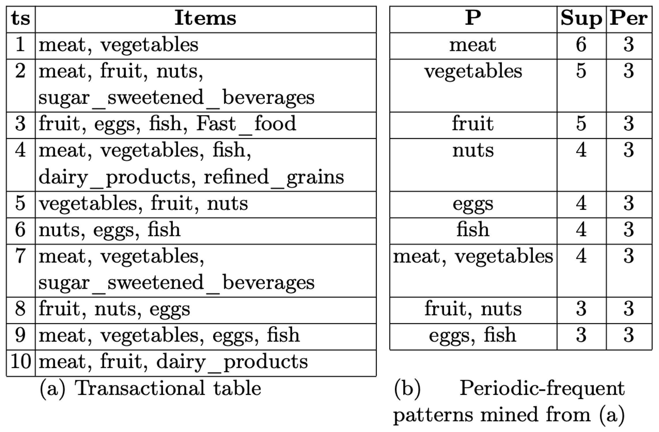
For example, the pattern meat, vegetables: [4, 3] expresses that if a 2-pattern happens (i.e., meat and vegetables are items of the pattern), then within three periods, it will appear again with a probability (or sup) of 3.
In general, if P A = { p a i } i = 1 . . L , where L is the number of mined patterns, is a set of mined patterns, the format of a mined pattern i t h is
p a i = ( { i t e m j } ) : [ s u p , m a x P e r ] .
Periodic-frequent pattern miningtries to discover all periodically occurring frequent patterns in a temporal database. In our research, we want to mine such periodic-frequent patterns from an uncertain temporal dataset, as mentioned before.
Let I = { I i } i = 1 . . N denote the itemset. Let T j = { I m } m [ 1 , N ] denote a transaction that is a set of items of the itemset. Let P k = { { I n } n [ 1 , N ] , support(%), periodicity(%)} denote a periodic-frequent pattern where the set of items { I n } n [ 1 , N ] has the frequency expressed by support(%), and how regularly this pattern appear within a database is depicted by periodicity (%).
The periodic-frequent pattern mining algorithm introduced by Uday et al. [13] gets { T j } j = 1 . . M , where M is the total transactions, as the input and generates { P k } k = 1 . . P , where P is the total patterns, as the output. The minSup (i.e., select only patterns with their support larger than minSup) and maxPer (i.e., choose only patterns with their periodicity smaller than maxPer) must be declared beforehand to limit the searching scope.
Figure 3 illustrates a toy sample of an itemset, transaction, and periodic-frequent patterns. The terms ts, P, Sup, and Per are acronyms of transaction, pattern, support, and periodicity, respectively. Readers could refer to the original paper [13] for more details.
We assume we have 10 receipts of customers from a small grocery in town, where each receipt records the list of food purchased by a customer. Then, we want to understand how frequently and periodically one food type is purchased. Figure 3a illustrates these 10 receipts; each receipt is considered as one transaction (ts). Figure 3b depicts the result from the periodic-frequent pattern mining. We can see that “meat” is bought with high frequency (i.e., 6/10), and after every three transactions, “meat” is repurchased.

2.3. Data Pre-Processing: Fuzzy Logic and Transactions

We apply fuzzy logic to discretize the data since we utilize a periodic-frequent pattern data mining algorithm to discover people’s daily nutrition and activity patterns with the aim of selecting valuable subsets of features to build a prediction model. The algorithm requires the input of the transactional table. Since the transactional table is built on point-wise data (i.e., itemset), we need to convert continuous values to level values. For example, the traditional transactional table of a supermarket problem contains a set of items (milk, vegetable, meat, bread), not the quantity of these items. Therefore, if we want to apply transactional tables to our data, we must convert them into item sets.
We decide to apply fuzzy logic with three levels to discretize the data. The reason for choosing three levels (low, medium, high) is to adapt human habits when talking about the quality of something. We can determine more levels (e.g., 5, 7); however, we found that three levels are enough to explain the cognition of people and more straightforward to explain the meaning of the patterns.
Since we pay attention to nutrition and physical activities, we first filter out irrelevant data, convert different measure units into one, and synchronize data by temporal dimension. Finally, we get a new dataset containing only cleaned nutrition and physical activities synchronized by timeline.
People have studied the association between food categories and calorie intake for a long time. Moreover, food categories also provide information on healthy and unhealthy meals that people should take for personal purposes. In [18,19,20], the authors provide food categories built upon different criteria (e.g., food colors, iodine, fast-food vs. slow-food, calorie intake). These studies offer a hint for us to create our food categories: (1) refined_grains, (2) vegetables, (3) fruits, (4) nuts, (5) eggs, (6) dairy_products, (7) fishes, (8) meats, (9) sugar_sweetened_beverages, and (10) fast_food. We first manually locate and determine the portion of each food category in each food image. Then, we apply fuzzy logic to divide each portion into one of the three levels of low (less than 20%), medium (between 20% to 50%), and high (over 50%). Finally, we attach these labels as the prefix of portion categories to generate the itemsets.
For example, there is a dish with whole grain bread, steamed broccoli, boiled egg, and strawberries. We assign categories “refined_grains”, “vegetables”, “eggs”, and “fruits”. Then, we estimate how large each category is compared to the whole dish. Suppose we have 55% of “refined_grains”, 30% of “vegetables”, 10% of “eggs”, and 5% of “fruits”; then, we will have a set of items {high_refined_grains, medium_vegetables, low_eggs, low_fruits} for the dish.
In [21], the authors provide interesting information related to US adults’ typical daily calorie needs by demographic and other characteristics. Hence, we can estimate the average calories for adults daily. Based on that, we define low (less than 2000 calories/day), medium (between 2000 to 3000 calories/day), and high (over 3000 calories/day) levels for the daily calorie intake for each person.
For the rest of the data types, we determine their levels based on popular criteria of the value ranges. Table 2 describes how we determine levels for each data types.
By adding the prefix “low”, “medium”, and “high” to each feature’s name associated with its value, we generate the itemset. Then, all items appearing during one person’s day are utilized to create a transaction set.

2.4. Feature Selection

Feature selection is one of the most critical stages in machine learning. It aims to reduce the data’s dimensionality and enhance any proposed framework’s performance [22]. Many feature selection works have been reported from various applications and domains. These reports converge into one common sense: feature selection suffers from many factors, such as high dimensionality, computational and storage complexity, noisy or ambiguous nature, and high performance, to name a few. Despite the challenges mentioned, feature selections bring undeniable benefits to enhance machine learning models’ productivity (e.g., accuracy, complexity).
This section discusses our feature selection mechanism, through which significant characteristics of a group and person are distributed into different discriminative sets. Our aim is to find a group of features that can leverage the common sense of one group’s members while maintaining the uniqueness of each member of that group. This could contribute to developing a supervised model that could start with a few samples shared by a group of people to generate a primary instance and end with an adaptive instance when considering personal characteristics.
Our hypothesis for feature selections is based on the following observations and facts.
  • People share common characteristics with their group and have personal characteristics that make them unique from a group.
  • With the same exercise and nutrition plan, finding two people with the same outcome is problematic.
  • People who prefer a self-training plan tend not to follow the plan strictly due to both subjective (e.g., tired, not in the mood) and objective reasons (e.g., busy working, unexpected meeting)
Based on the discussions above, we created three personal, intersection, and general features, where the first describes the uniqueness of one person, the second indicates the common concrete characteristics shared inside one group, and the third is involved in characteristics that two people at least share in a group.
It should be noted that we rely heavily on the periodic-frequent pattern mining results to build these three feature types. In other words, we consider people’s habits and frequency of data factors, both for individuals and groups.

2.4.1. Personal Features

For each person, we apply periodic-frequent pattern mining to the relevant transactional dataset as explained in Section 2.3. Based on the output of the pattern mining, we select all patterns with high frequency (i.e., support) or high periodicity. In other words, we are interested in patterns that appear frequently and at regular intervals or rarely appear within the data. The union of these patterns provides a compact and discriminative feature set representing one person. Let P F i denote the feature set of person p i .

2.4.2. Intersection Features

We take the intersection of relevant { P F i } for each group I P F = { P F i } . We hypothesize that the intersection features I P F represent the very discriminative characteristic among people in the same group. We believe that I P F has strong discrimination to distinguish a group from others.

2.4.3. General Features

We take the union of relevant { P F i } for each group U P F = { P F i } . We hypothesize that people still belong to a group, even though they have some points that differ from other group members, as long as they share the discriminative characteristic of the group.

2.5. The Data-Driven Stacking-Based Model

To utilize three different feature sets ideally, as mentioned above, we decided to use the stacking learning approach [23], which allows several “weak learners” to be combined into one “strong learner” in the end. That is because we want to balance the generalization and personalization of our prediction model so that it can leverage not only group data but also personal data.
In this work, we choose the stacking-based model [24] because it frequently takes weak learners into account in a heterogeneous manner, teaches them concurrently, and combines them by training a composite model to create a robust prediction model.
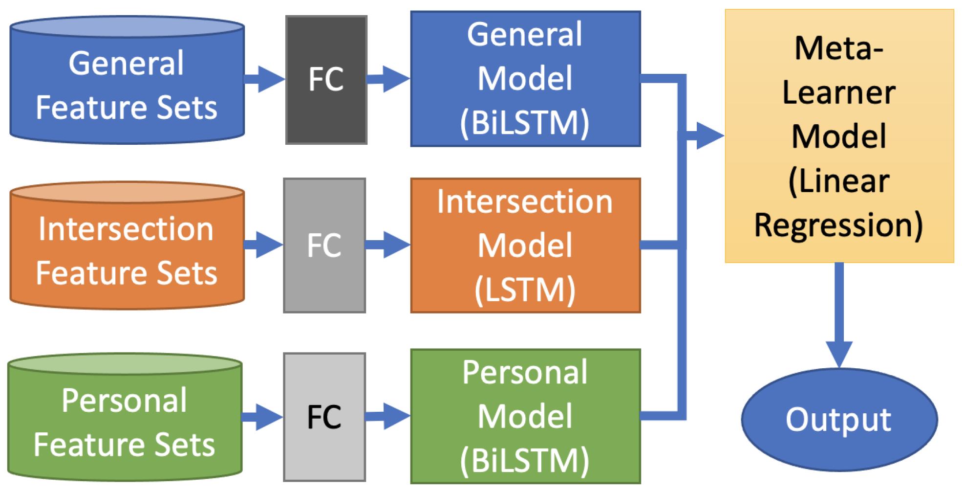
As depicted in Figure 4, we create three models associated with three feature sets. We use a BiLSTM model for general and personal feature sets and a standard LSTM for the intersection feature set. We use the full connection (FC) to normalize input data dimensions and enhance salient training features.
We choose BiLSTM for general and personal models and LSTM for the intersection model because BiLSTM can exploit and explore the context and utilize information from both directions (e.g., forward, backward); hence, it could compensate for the asymmetric nature of general and personal features. In contrast, the intersection feature set is symmetric, and we can apply the indirect flow of LSTM without losing any significant cues.
The primary idea of using the stacking model here is that we do not ensure which model and feature set can give the best result. Hence, we need to estimate the weight set by which the balance of outputs from the three models can be reached so that the final output can achieve the highest accuracy. Moreover, depending on different circumstances, we can quickly and flexibly switch the output levels from stacking mode to personal/general/intersection mode to adapt our model to local datasets. Besides, this could support us in adjusting the computational workload and volume of data.

3. Experimental Results

We utilize the PMData dataset to evalute our model. Firstly, we conduct data pre-processing, including cleaning, polishing, and grouping of data. Secondly, we generate the itemset using fuzzy logic to construct transactional data for each person. Thirdly, we mine these transactional data to produce a periodic-frequent pattern set for each person. Fourthly, we create general, intersection, and personal feature sets for each group. Finally, we train, validate, and test our models accordingly.
Since the weight loss and running speed are reported in numeric format, we decided to use MAE and MSE as the metrics for evaluation. We use MAE to measure the accuracy and MSE to evaluate the sensitivity with outliers of our models.

3.1. Data Grouping

We hypothesize that our feature selection approach can alleviate the dependence on the data grouping strategy. We conduct our model on the full dataset and data groups made by different clustering strategies to prove our hypothesis. This subsection introduces how we divide data into different group types.
We cluster the dataset into various groups according to different criteria. The clustering is based on the hypothesis that if people are grouped based on some common factors (e.g., demographic data, habits, food interests), their data will be discriminative compared to others. Table 3 denotes data groups and related criteria used for grouping.
We use the prefixes “weight” and “speed” to denote the categories we have to predict—change in weight and change in running speed—and the rest of each name expresses the group criteria. For example, “Speed_Group_A” denotes a group for predicting running speed change in which people generally wake up early (potentially also go to bed early, i.e,. type A in PMData), or “Weight_Group_Age_20_40_Male” describes a group for predicting weight change where people must be male and between 20 and 40 years of age.

3.2. Evaluations

Table 4 shows that our model produces accuracy with a low MAE (<0.5) and MSE (<0.4) in all groups (also compared to other often-used methods later in the article). Among models, the stacking model gives the best accuracy. Interestingly, we can see that the food images significantly strengthened the accuracy level, even though only three people took food pictures.
There is an exciting observation of group “AAA_group_image_food” where the stacking model generates a better accuracy for the “weight” group than the “speed” group. This observation strengthens the role of nutrition in training performance: if you have a good nutrition regimen (both in healthy qualifications and regular meals eaten), you can improve your training performance. Another important and interesting discovery is that though people record the calories they took during the day, the food images they took are more informative.
From the observations mentioned, we discovered the following interesting facts: (1) to predict running speed change, we should focus on a group’s common features rather than individual features; (2) to predict weight change, we must consider both common and individual features; and (3) to achieve high accuracy for each person, we have to use both common and individual features.
The final interesting observation is that our model can work well with different groups (i.e., using the entire data cohort or particular group data, the model still predicts well). Hence, our model can work independently with subjective clustering defined by individual people. This discovery is beneficial when applying our model to a new cohort because it means one does not need to worry about how to divide the data into suitable groups. This validates the idea that our feature selection approach can alleviate the problem of data grouping. Moreover, it points out that exercise outcomes are associated with daily habits, not people’s demographic characteristics.
Table 5 denotes some interesting patterns mined from the data of participant P03. We can consider this person as not active looking at the frequency of “not exercise” activities, which occupy a large portion of the data. Further, this person has a habit of drinking a lot of water regularly. In addition, this person has the habit of eating fast food (not in large portions, but regularly). The prediction results of a change in running speed and weight for this person are accurate, forecasting a weight increase and slower running speed. Together with the periodic-frequent patterns mined from this person’s lifelogs, we can see the interesting correlation between nutrition, physical activities, and training performance. Based on that, the person could be recommended to adjust their food intake and activity level to achieve possible weight loss. This detailed example shows that our method can be used to provide recommendations based on the data and predictions, which could lead to possible health and performance benefits.

3.3. Comparisons

We compare our model to other models tested on the same dataset to obtain more objective evaluations. We select three models for this comparison: (1) the personalized adaptive model [25], (2) the Vanilla LSTM model [26], and (3) a one-dimensional convolutional neural network (CNN1D) model [26]. The first model also considers general and personal feature sets and applies a correlation matrix to select common and individual features. The purpose of this model is to predict sleeping quality using lifelog data. The second and third models use the whole dataset, not separating data into different groups. The target of these models is the same as ours.
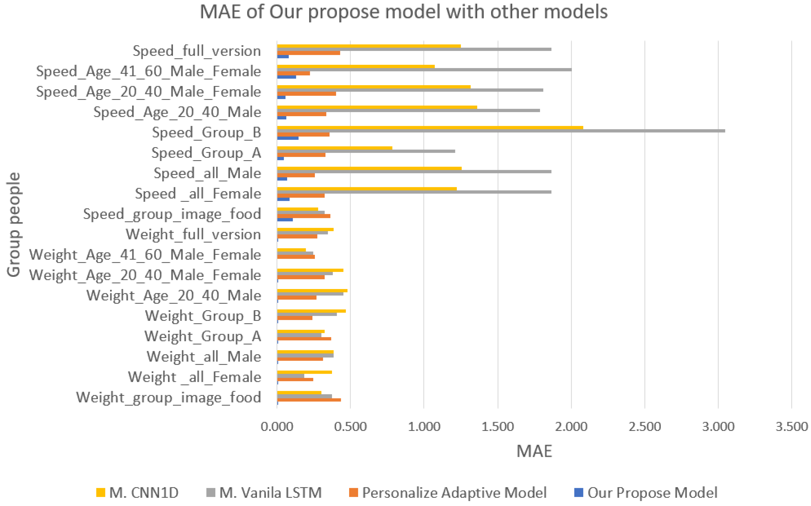
Figure 5 illustrates the comparison between the personalized adaptive, CNN1D, and Vanilla LSTM models and our approach using the MAE metric. We can see that our model almost beats the adaptive model. The adaptive model utilizes a correlation matrix to group all high-correlation data factors with sleep quality and assumes that these data factors can influence sleep quality. Based on that, the researchers hope they can understand and predict sleep quality by monitoring the changes of these data factors. When applying this model to the PMData dataset, we guess that the correlation data factors are less discriminative than our feature sets that pay attention to intra and inter-correlation among people.
We also see that considering both group and individual datasets provides better accuracy than using the entire dataset. The personalized approach and our model work better than CNN1D and Vanilla LSTM, which deal with the whole dataset.

4. Conclusions and Future Works

In this paper, we introduce a method for indicating training performance for amateur athletes using nutrition and activity lifelogs. We apply the fuzzy logic to discrete data and transform them into transactional data, with which we can apply the periodic-frequent pattern mining technique to extract discriminative feature sets, i.e., union (general), intersection, and personal. We build a data-driven stacking-based model based on these feature sets to strengthen three weak learners with related feature sets. We evaluate our method on different groups that are divided subjectively using demographic data. We also compare our models to three other methods on the same dataset and metrics. The results show a comparable accuracy in addition to the exciting insights discovered with our approach.
In the future, we plan to develop a tool to detect food categories automatically. We will also compare the benefit of using correlation and pattern mining to establish discriminative feature sets. We will apply our approach to predict other factors such as sleep qualification, stress, and eating and drinking habits. We also intend to discover the relationship or association between nutrition and activity lifelogs with other factors.

Author Contributions

Project administration and conceptualization, M.-S.D., writing—review and editing, P.-T.N., M.A.R., R.U.K., T.-T.D., D.-D.L., K.-C.N.-L., T.-Q.P. and V.-L.N. All authors have read and agreed to the published version of the manuscript.

Funding

This research is funded by the University of Economic Ho Chi Minh City (UEH) Vietnam grant number 2022-09-19-1159.

Data Availability Statement

The data of this research can be found at: https://datasets.simula.no/pmdata/ (accessed on 18 December 2022).

Acknowledgments

We acknowledge the University of Economic Ho Chi Minh City (UEH) for funding this research.

Conflicts of Interest

The authors declare no conflict of interest. The funders had no role in the design of the study; in the collection, analyses, or interpretation of data; in the writing of the manuscript; or in the decision to publish the results.

References

  1. Rothschild, J.A.; Kilding, A.E.; Plews, D.J. Pre-exercise nutrition habits and beliefs of endurance athletes vary by sex, competitive level, and diet. J. Am. Coll. Nutr. 2021, 40, 517–528. [Google Scholar] [CrossRef] [PubMed]
  2. Thompson, W.R. Worldwide survey of fitness trends for 2020. ACSMs Health Fit. J. 2019, 23, 10–18. [Google Scholar] [CrossRef]
  3. Singh, V.N. A Current Perspective on Nutrition and Exercise. J. Nutr. 1992, 122, 760–765. [Google Scholar] [CrossRef] [PubMed]
  4. Sun, W. Sports Performance Prediction Based on Chaos Theory and Machine Learning. Wirel. Commun. Mob. Comput. 2022, 2022, 3916383. [Google Scholar] [CrossRef]
  5. Iyer, S.R.; Sharda, R. Prediction of athletes performance using neural networks: An application in cricket team selection. Expert Syst. Appl. 2009, 36, 5510–5522. [Google Scholar] [CrossRef]
  6. Ragab, N. Soccer Athlete Performance Prediction Using Time Series Analysis. Master’s Thesis, OsloMet-Storbyuniversitetet, Oslo, Norway, April 2022. [Google Scholar]
  7. Zhou, L.; Gurrin, C. A survey on life logging data capturing. In Proceedings of the SenseCam Symposium 2012, Oxford, UK, 3–4 April 2012. [Google Scholar]
  8. Gurrin, C.; Zhou, L.; Healy, G.; Jónsson, B.Þ.; Dang-Nguyen, D.; Lokoč, J.; Tran, M.; Hürst, W.; Rossetto, L.; Schöffmann, K. Introduction to the Fifth Annual Lifelog Search Challenge. In Proceedings of the 2022 International Conference on Multimedia Retrieval (LSC’22), Newark, NJ, USA, 27–30 June 2022. [Google Scholar]
  9. NII. NII Testbeds and Community for Information Access Research. Available online: https://research.nii.ac.jp/ntcir/index-en.html (accessed on 18 December 2022).
  10. Ninh, V.-T.; Le, T.-K.; Zhou, L.; Piras, L.; Riegler, M.; Halvorsen, P.L.; Tran, M.-T.; Lux, M.; Gurrin, C.; Dang-Nguyen, D.-T. Overview of ImageCLEF Lifelog 2020: Lifelog Moment Retrieval and Sport Performance Lifelog. In Proceedings of the CLEF2020 Working Notes, Ser. CEUR Workshop Proceedings, Thessaloniki, Greece, 22–25 September 2020; Available online: http://ceur-ws.org (accessed on 18 December 2022).
  11. Chung, S.; Jeong, C.Y.; Lim, J.M.; Lim, J.; Noh, K.J.; Kim, G.; Jeong, H. Real-world multimodal lifelog dataset for human behavior study. ETRI J. 2021, 44, 426–437. [Google Scholar] [CrossRef]
  12. Thambawita, V.; Hicks, S.A.; Borgli, H.; Stensland, H.K.; Jha, D.; Svensen, M.K.; Pettersen, S.A.; Johansen, D.; Johansen, H.D.; Pettersen, S.D.; et al. PMData: A sports logging dataset. In Proceedings of the 11th ACM Multimedia Systems Conference (MMSys ’20), Istanbul, Turkey, 8–11 June 2020; Association for Computing Machinery: New York, NY, USA, 2020; pp. 231–236. [Google Scholar]
  13. Kiran, R.U.; Kitsuregawa, M.; Reddy, P.K. Efficient discovery of periodic-frequent patterns in very large databases. J. Syst. Softw. 2016, 112, 110–121. [Google Scholar] [CrossRef]
  14. Chatterjee, A.; Prinz, A.; Riegler, M. Prediction Modeling in Activity eCoaching for Tailored Recommendation Generation: A Conceptualization. In Proceedings of the 2022 IEEE International Symposium on Med-ical Measurements and Applications (MeMeA), Messina, Italy, 22–24 June 2022; pp. 1–6, ISBN 978-1-6654-8299-8. [Google Scholar] [CrossRef]
  15. Karami, Z.; Hines, A.; Jahromi, H. Leveraging IoT Lifelog Data to Analyse Perfor-mance of Physical Activities. In Proceedings of the 2021 32nd Irish Signals and Systems Conference (ISSC), Athlone, Ireland, 10–11 June 2021; pp. 1–6, ISBN 978-1-6654-3429-4. [Google Scholar] [CrossRef]
  16. Diaz, C.; Caillaud, C.; Yacef, K. Unsupervised Early Detection of Physical Ac-tivity Behaviour Changes from Wearable Accelerometer Data. Sensors 2022, 22, 8255. [Google Scholar] [CrossRef] [PubMed]
  17. Kazuki, T.; Dao, M.; Zettsu, K. MM-AQI: A Novel Framework to Understand the Associations Between Urban Traffic, Visual Pollution, and Air Pollution. In Proceedings of the IEA/AIE, Kitakyushu, Japan, 19–22 July 2022; pp. 597–608. [Google Scholar]
  18. Haldimann, M.; Alt, A.; Blanc, A.; Blondeau, K. Iodine content of food groups. J. Food Compos. Anal. 2004, 18, 461–471. [Google Scholar]
  19. Schwingshackl, L.; Schwedhelm, C.; Hoffmann, G.; Knuppel, S.; Preterre, A.L.; Iqbal, K.; Bechthold, A.; Henauw, S.D.; Michels, N.; Devleesschauwer, B.; et al. Food groups and risk of colorectal cancer. IJC J. 2017, 142, 1748–1758. [Google Scholar] [CrossRef] [PubMed] [Green Version]
  20. 7ESL Homepage. 2022. Available online: https://7esl.com/fast-food-vocabulary/ (accessed on 18 December 2022).
  21. McKinnon, R.A.; Oladipo, T.; Ferguson, M.S.; Jones, O.E.; Maroto, M.E. Beverly Wolpert Reported Knowledge of Typical Daily Calorie Requirements: Relationship to De-mographic Characteristics in US Adults. J. Acad. Nutr. Diet. 2019, 119, 1831–1841.e6. [Google Scholar] [CrossRef] [PubMed]
  22. Dhal, P.; Azad, C. A comprehensive survey on feature selection in the various fields of machine learning. Appl. Intell. 2022, 52, 4543–4581. [Google Scholar] [CrossRef]
  23. Berk, R.A. An Introduction to Ensemble Methods for Data Analysis. SAGE J. 2006, 34. [Google Scholar] [CrossRef] [Green Version]
  24. Wang, J.; Liu, C.; Li, L.; Li, W.; Yao, L.; Li, H.; Zhang, H. A Stacking-Based Model for Non-Invasive De-tection of Coronary Heart Disease. IEEE Access 2020, 8, 37124–37133. [Google Scholar] [CrossRef]
  25. Van, N.T.P.; Son, D.M.; Zettsu, K. A Personalized Adaptive Algorithm for Sleep Quality Prediction using Physiological and Environmental Sensing Data. In Proceedings of the IEEE 2021 8th NAFOSTED Conference on Information and Computer Science (NICS), Hanoi, Vietnam, 21–22 December 2021. [Google Scholar]
  26. Mai-Nguyen, A.V.; Tran, V.L.; Dao, M.S.; Zettsu, K. Leverage the Predictive Power Score of Lifelog Data’s Attributes to Predict the Expected Athlete Performance. In Proceedings of the CLEF, Thessaloniki, Greece, 22–25 September 2020. [Google Scholar]
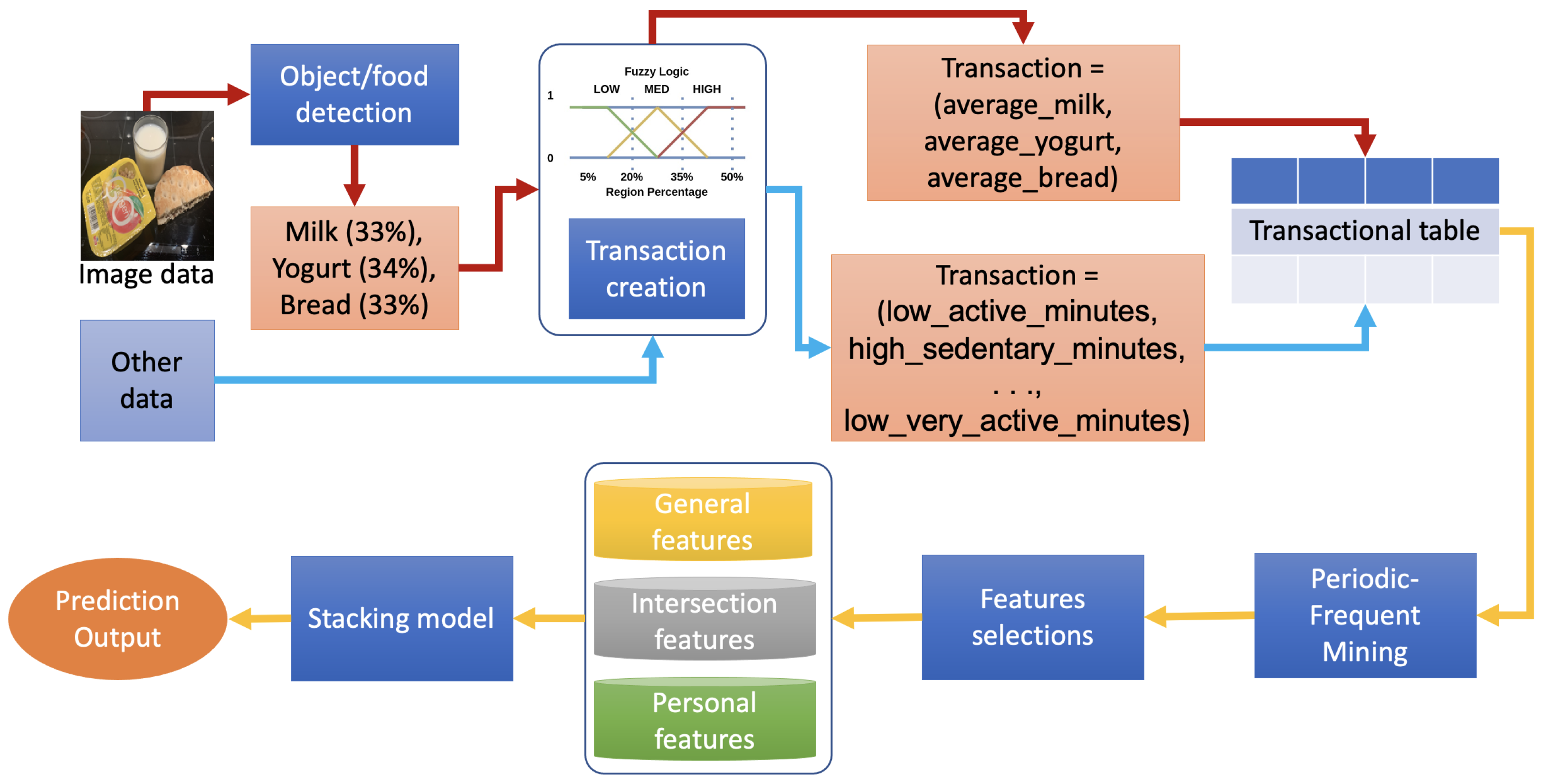
Figure 1. The method’s overview.
Algorithms 16 00030 g001
Figure 2. Examples of the captured food and drinks images [12].
Algorithms 16 00030 g002
Figure 3. A toy example of periodic-frequent patterns mining.
Algorithms 16 00030 g003
Figure 4. The data-driven stacking-based Model: an overview.
Algorithms 16 00030 g004
Figure 5. Comparing the proposed model with others.
Algorithms 16 00030 g005
Table 1. Overview of the PMData dataset [12].
CategoriesFileRate of EntriesNumber of Entries
SRPEsrpe.csvPer exercise783
Injuryinjury.csvPer week225
Wellnesswellness.csvPer day1747
Stepssteps.jsonPer minute1,534,705
Caloriescalories.jsonPer minute3,377,529
Distancedistance.jsonPer minute1,534,705
Exerciseexercise.jsonWhen it happens (100 entries per file)2440
Heart rateheart_rate.jsonPer 5 s20,991,392
Lightly active minuteslightly_active_minutes.jsonPer day2244
Sedentary minutessedentary_minutes.jsonPer day2396
Moderately active minutesmoderately_active_minutes.jsonPer day2396
Very active minutesvery_active_minutes.jsonPer day2396
Resting heart rateresting_heart_rate.jsonPer day1803
Sleepsleep.jsonWhen it happens (usually daily)2064
Sleep scoresleep_score.csvWhen it happens (usually daily)1836
Time in heart rate zonestime_in_heart_rate_zones.jsonPer day2178
Google Forms reportingreporting.csvPer day1569
Table 2. Data Level Determination.
FeaturesLow LevelNormal LevelHigh Level
Calories_all_day0–20002000–30003000–6000
exercise_calories0–200200–450450–6000
distance0–70007000–90009000–25,000
exercise_distance0–40004000–70007000–25,000
lightly_active_minutes0–18001800–21002100–42,000
exercise_lightly_minutes0–18001800–21002100–42,000
steps0–10,00010,000–18,00018,000–30,000
exercise_steps0–20002000–40004000–30,000
moderately_active_minutes0–63006300–69009000
exercise_moderately_minutes0–63006300–69009000
sedentary_minutes0–600600–18001800–90,000
exercise_sedentary_minutes0–600600–18001800–90,000
very_active_minutes0–15,00015,000–15,60015,600–120,000
exercise_very_minutes0–15,00015,000–15,60015,600–120,000
exercise_averageHeartRate0–9595–170170–2000
exercise_speed0–77–99–15
exercise_duration0–15001500–21002100–9000
time_per_kilometer0–15001500–21002100–9000
exercise_elevationGain0–1515–100100–300
exercise_heartRateZones_FatBurn_minutes0–36003600–51005100–120,000
exercise_heartRateZones_Peak_minutes0–11,22011,220–12,00012,000–30,000
exercise_heartRateZones_Cardio_minutes0–61806180–75007500–30,000
Table 3. Data grouping.
Name of GroupPerson in Group
Weight_Group_Image_foodp01, p03, p05
Weight_all_Femalep04, p10, p11
Weight_all_Malep01, p02, p03, p05, p06, p07, p08, p09, p12, p13,
p14, p16
Weight_Group_Ap01, p02, p03, p04, p05, p11, p12, p13, p14
Weight_Group_Bp06, p07, p08, p09, p10, p16
Weight_Group_Age_20_40_Male
p16
p03, p05, p06, p07, p08, p09, p12, p13, p16
Weight_Group_Age_20_40_Male_and_Femalep03, p04, p05, p07, p08, p09, p10, p11, p12, p13,
p16
Weight_Group_Age_41_60Male_and_Femalep01, p02, p06, p14
Weight_all_peoplep01, p02, p03, p04, p05, p06, p07, p08, p09, p10,
p11, p12, p13, p14, p16
Speed_Group_Image_foodp01, p03, p05
Speed_all_Femalep04, p10, p11
Speed _all_Malep01, p02, p03, p05, p06, p07, p08, p09, p12, p13,
p14
Speed _Group_Ap01, p02, p03, p04, p05, p11, p12, p13, p14
Speed _Group_Bp06, p07, p08, p09, p10
Speed _Group_Age_20_40_Malep03, p05, p06, p07, p08, p09, p12, p13
Speed _Group_Age_20_40_Male_and_Femalep03, p04, p05, p07, p08, p09, p10, p11, p12, p13
Speed _Group_Age_41_60Male_and_Femalep01, p02, p06, p14
Speed_all_peoplep01, p02, p03, p04, p05, p06, p07, p08, p09, p10,
p11, p12, p13, p14
Table 4. Evaluation results of the data-driven stacking-based model.
Name of GroupGeneral ModelIntersection ModelPersonal ModelStacking Model
MAEMSEMAEMSEMAEMSEMAEMSE
Weight_group_image_food0.4160.2560.4080.2350.4580.3670.0060.002
Weight _all_Female0.3780.1980.3660.1810.2210.0720.0090.005
Weight_all_Male0.3220.1380.3760.1670.3910.2370.0030.001
Weight_Group_A0.4590.2480.4800.2360.2800.1500.0020.001
Weight_Group_B0.2380.0900.5090.2900.2370.0880.0070.003
Weight_Age_20_40_Male0.3710.1690.4430.2050.2250.0750.0050.001
Weight_Age_20_40_Male_Female0.3720.1880.4280.1900.2650.1300.0060.002
Weight_Age_41_60_Male_Female0.2700.1270.2930.1220.2030.0610.0000.000
Weight_full_version0.2310.0820.3710.1580.2630.1220.0050.002
Speed_group_image_food0.1690.0390.1260.0240.2250.0860.1070.020
Speed _all_Female0.1820.0510.1020.0210.3310.1520.0860.018
Speed_all_Male0.1340.0310.0780.0140.3490.1810.0670.012
Speed_Group_A0.1120.0230.0570.0110.3870.1820.0490.009
Speed_Group_B0.1750.0430.1710.0340.4630.2860.1450.029
Speed_Age_20_40_Male0.1500.0370.0730.0120.4540.2470.0620.010
Speed_Age_20_40_Male_Female0.1110.0210.0690.0090.4210.2170.0580.007
Speed_Age_41_60_Male_Female0.1510.0380.2530.0770.3220.1530.1280.033
Speed_full_version0.1190.0240.0950.0160.3450.1700.0810.013
Table 5. Periodic-frequent pattern mining results for participant P03.
PatternsSupport (%)Periodicity (%)
low_moderately_active_minutes,
high_sedentary_minutes,
low_very_active_minutes
0.992
low_glasses_of_fluid0.966
Yes_Breakfast, Yes_Dinner0.3716
high_Fast_food0.1424
Disclaimer/Publisher’s Note: The statements, opinions and data contained in all publications are solely those of the individual author(s) and contributor(s) and not of MDPI and/or the editor(s). MDPI and/or the editor(s) disclaim responsibility for any injury to people or property resulting from any ideas, methods, instructions or products referred to in the content.