1. Introduction
The presence of mass attachments in structural elements such as beams and columns is quite common in civil engineering infrastructure, as is the case with pylons supporting cables, wind turbines, antennas, lights, etc., [
1]. In certain cases, these mass attachments may vary with time on a scale comparable to that of the duration of the external dynamic loads. This may occur under certain conditions, as for example if the mass attachment plays the role of a damping device [
2]. Specifically, pylons are infrastructure components serving a variety of functions and can be efficiently modeled as waveguides [
3]. The presence of attachments on pylons leads to the concept of secondary systems, which may serve as passive or semi-active structural control devices, a typical example being liquid column dampers [
4]. Furthermore, the attached mass may in turn be connected to a nonlinear spring which acts as a vibration absorber [
5]. In general, it is possible to view the pylon with an attached time-variable mass as a system comprising a primary linear oscillator and a nonlinear secondary system. Much work has been done in this field from a mechanical engineering viewpoint, where the secondary system is often viewed as a Vibro-impact nonlinear energy sink [
6]. As a consequence, new methods of solving the problem must be sought, such as multiple-scale expansions, which are possible for low mass ratios of the combined primary-secondary system. For heavily attached masses that are also time-dependent, recourse must be made to alternative techniques [
7]. Here, we solve for the time-dependent, heavy top mass on a beam element by developing a technique based on a method originally outlined in [
8] and further improved in [
9], whereby the free vibration boundary-value problem (BVP) of a beam with point masses is reduced to an eigenvalue problem through the separation of variables, but the characteristic equation involving transcendental functions is bypassed.
Instead, the solution is expanded in series involving the eigenfunctions of the beam without any attachments, plus a new set of generalized coordinates which can be recovered from the solution of single-degree-of-freedom (SDOF) equations with generalized forces at the right-hand side (RHS) that correspond to the point masses. An additional complication arises when ground vibrations are considered because the motion of an attached mass on the pylon cannot be uncoupled by modal analysis, since the absolute accelerations experienced by the mass require contributions from all modes at the same instant [
10]. This necessitates a second-stage modal analysis, and if the attached mass is time-dependent, then the new eigen properties of the combined system are time-dependent since they are influenced by the mass rate of change [
7]. Based on this solution methodology, the transient pylon vibrations can be Fourier transformed to extract the time dependence of the eigenfrequencies of the combined pylon-mass system.
The usual model for pylons is based on the Bernoulli–Euler fourth-order differential equation for bending, or second order differential equations for axial and torsional responses [
3]. For an effective modelling of the lumped mass, it is necessary to introduce generalized functions [
11], also known as Schwartz distributions, making it possible to differentiate functions whose derivatives do not exist in the classical sense. In this work, the inertia term that develops at the top of the beam is a temporal discontinuity, and the Dirac delta function appears as a force term on the RHS of the differential equation under study. It is noted that the Dirac delta function can also be used to model the presence of a crack in a structural member, which reduces stiffness and alters the dynamic response [
12].
From the above discussion, it follows that a computationally demanding problem arises with the presence of point mass attachments in flexible structures. More specifically, the numerical complication arises from the fact that the point mass attachment is theoretically singular in space and may also exhibit a temporal singularity if the mass suddenly increases or decreases with time. Furthermore, if the magnitude of the mass attachment is large as compared to the mass of the supporting pylon, then the dynamic properties of the combined structural system change compared to the original, stand-alone beam. Thus, a time-dependent eigenvalue problem arises, which must be solved in either a direct or an iterative way, for every time step until the complete duration of the vibrations is covered. An additional issue is that the equations of motion yield an eigenvalue formulation that includes a non-symmetric damping matrix, which in turn renders the eigenvalues as complex quantities. Focusing on the eigenvalue analysis of the combined pylon-mass system, the coefficients of the polynomial resulting from setting the determinant of the system matrix equal to zero are recovered using the Leverrier–Faddeev algorithm [
13]. Subsequently, two eigenvalue extraction methods are examined, namely the Laguerre method, which is the complex number variant of the conventional Newton–Raphson method used for real root extraction [
14,
15], and the QR method [
16] in conjunction with the Householder algorithm [
16].
Once the eigenvalue problem has been solved and followed by synthesis of the transient response of the pylon-mass system [
17], then it is possible to proceed to system identification, either as a stand-alone endeavor or within the context of structural health monitoring (SHM). Typically, this entails extracting information based on the dynamic response of the monitored structure. Standard practice [
18] utilizes the free vibration regime, but here the short-term Fourier transform (STFT) of the forced vibration regime is used to trace the time evolution of dominant eigenfrequencies of a pylon with a time-variable mass attached at the top. The external forcing functions are harmonic ground motion, and two cases are considered, one where the mass decreases to a nearly zero value starting from a reference value, plus the opposite case where the additional mass increases from zero to the same reference value, which can be substantial, i.e., reaching 20% of the pylon mass. These eigenfrequencies converge to the standard values computed when the additional mass has a fixed value when ground motion ceases. The methodology presented herein is useful in extracting as much information as possible from dynamic responses for use in the SHM of typical civil engineering infrastructure ranging from pylons to bridges and buildings [
19].
2. Non-Autonomous Dynamic Systems
In terms of the dynamic response of structural systems, the presence of attachments that lead to passive and/or active control adds terms to either the differential operator or the boundary conditions. This situation, however, presupposes that the mass and stiffness parameters of the structural system remain time-invariant [
20], i.e., the system is autonomous. If this is not the case and these parameters are time-dependent, then the structural system is labeled as non-autonomous [
21]. The pylon with the attached transient mass studied here belongs to the latter group, and the target is to move the eigenfrequencies of the combined system away from the dominant frequency range of the externally applied excitations [
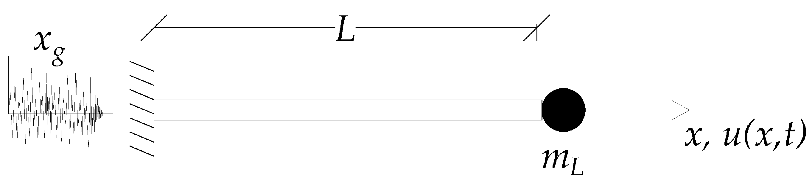
7]. In what follows, we focus on the longitudinal vibrations of the supporting pylon, although the methodology can be extended to cover transverse vibrations as well.
2.1. Equation of Motion for Longitudinal Vibrations
The equation of motion and boundary conditions [
3] for a cantilevered pylon of length
L with a time-varying, lumped mass attachment
at the top
and undergoing longitudinal vibrations, see
Figure 1, are given below as follows:
In the above,
E is the modulus of elasticity,
A is the cross-section area, and
ρ is the material density of the pylon for a continuous mass distribution. Next,
is the displacement along the x-axis and
is the time-dependent ground motion imparted at the base, with primes (′) and dots
respectively denoting spatial and temporal derivatives. Moreover, initial conditions are assumed to be zero. It should be noted that the boundary conditions in Equation (1) have been rendered homogeneous by absorbing the lumped mass inertia effects
in the equation of motion using the Dirac delta function
. This however changes the eigenvalue problem of the original stand-alone pylon to a more complicated one and requires an additional investigation as to the number of terms required for convergence for a modal analysis [
17]. Note that the presence of a point discontinuity at boundary
poses a more stringent convergence requirement as compared to the case of the discontinuity appearing in the interior
of the waveguide.
2.2. The Dirac Delta Distribution
The definition of the Dirac delta function
given below is heuristic, in the sense that this is not a proper function [
22], but can be defined as either a measure or as a distribution:
Listed below are the translation identity and its limiting form for weight function
as two stations,
and
, coalesce:
2.3. Steel Pylon with Attached Mass
The steel pylon shown in
Figure 1 is a circular cylinder with a constant cross-section, fixed at the base and with a time-varying mass attached at the top. The latter element can be considered as a tank with a valve permitting the inflow and outflow of a liquid, e.g., water. The properties of this combined structural system are listed in
Table 1. Two scenarios are considered, the first for the water tank at the top being filled up from an initial mass ratio
(nearly empty) to a mass ratio
(full) with a flow rate
. The second scenario is the reverse, starting from
and dropping to
with a flow rate
. The time scale required for each of these processes to be completed is
The external force is a harmonic ground motion with a displacement amplitude of
.
2.4. Dynamic Response of the Steel Pylon
Following the transposition of the attached mass inertia terms to the equation of motion, the eigenvalue problem for the pylon is now defined at time
, where a fixed mass
has been placed at the top end
. The characteristic equation for the pylon modeled as a waveguide under axial vibrations with the boundary condition
is:
In the above, the mass ratio is defined as
, with
the mass of the stand-alone pylon and
is the corresponding wave number. Equation (2) can be solved numerically to recover the eigenfrequencies in two stages, starting with the bisection method to extract the roots, and followed by Newton–Raphson for better convergence [
14].
Given the formulation in Equation (1), separation of variables is possible and therefore the following expansion is obtained
where
is the eigenfunction and
is the generalized coordinate. Note that the summation convention is implied for repeated indices. For the stand-alone, cantilevered pylon, the eigenfunctions are given [
10] as
.
2.5. Eigenvalue Problem Formulation
The eigenvalue problem is first expressed in terms of the aforementioned generalized coordinates
, for
eigenvalues, which are deemed sufficient in the analysis, as follows:
In the above, [
M(t)], [
C], and [
K] are the mass matrix, a damping–type matrix and the stiffness matrix, respectively, written in a normalized form. Two mass ratios are defined here as
(dimensionless) and
(a normalized mass rate). Furthermore,
[rad/s] are the eigenfrequencies of the stand-alone pylon. In order to recover a closed-form solution, we proceed to recast the above second-order, matrix differential equation as a first-order differential equation of double size as
The more compact form for the above matrix equation is
At this point, we opted for a time-stepping solution of Equation (8) by defining a total time interval of interest as , with N the total number of time steps Δt. Thus, is the time it takes for the mass ratio to commence from an initial value and reach a final value. During a given time instant , the system matrix is assumed to remain constant. Once the number of eigenvalue/eigenfunction pairs has been decided upon (in our case, ), the eigenvalue problem is solved starting at time with . This is continued for all time steps with system matrix , and initial conditions equal to the final conditions for the displacement and velocity of the immediately previous time step .
In more detail, since system matrices [
A(t)], [
B(t)] are symmetric, a solution in the form
, where the carat indicates the amplitude of the kinematic variables, namely of the displacement and velocity. Upon substitution in Equation (8), the eigenvalue problem assumes its standard form as follows:
Solution yields the complex-valued eigenvalues
. Specifically, the condition
yields
Since the first of the above equations is merely an identity, we impose on the second one the determinant equal to zero as
. This is the equation that can now be solved for every time increment from the onset of motion at
. The time-dependent eigenvalue code is depicted in
Table 2 and all computations were carried out using the Python [
23] software.
Assembly and solution using the 2
N × 2
N matrix
for a given time step, see Equation (9):
|
|
|
|
|
|
|
| |
|
|
|
|
|
|
|
|
|
|
|
|
|
|
|
3. Eigenvalue Extraction for Non-Autonomous Dynamic Systems
The general form of the eigenvalue problem is shown below, from which it is possible to recover the eigenvalues as the roots of the polynomial
that results from setting the determinant of the matrix system equal to zero:
The first step in the solution of the characteristic equation which emerges from Equation (11) requires the computation of the coefficients of the resulting polynomial. This is achieved by using the Leverrier–Faddeev algorithm [
24], which produces a sequence of successive matrices replacing
until it becomes diagonal and then computes its trace as the sum of the diagonal terms. The trace is then used as input for the Laguerre algorithm [
25] and the output is
pairs of complex conjugate roots, where
is the number of eigenmodes retained in the representation of the dependent variable, see Equation (5):
In the above,
(rad/s) are the damped eigenfrequencies of the stand-alone pylon for Rayleigh damping, with
the viscous damping ratio. In order to recover real-valued eigenfrequencies (in
) from Equation (12), the amplitude of
is divided by
, resulting in
3.1. The Laguerre Method
Laguerre’s method [
25] expresses a polynomial of order
in a recursive form as
The derivatives of the polynomial are computed as
Thus, bringing the polynomial in the form
it becomes obvious that there is a root at
and there are
roots at
. The next step is to take the derivative of Equation (16) as
Following that, one proceeds with the second derivative:
By defining
and manipulating terms finally yields the recursive Laguerre formula for root
is as follows:
The improved root determined by choosing the sign results in the larger magnitude of the denominator.
3.2. The Leverrier–Faddeev Method
For the purpose of numerical implementation,
Table 3 below gives the structure of the Leverrier–Faddeev algorithm, which accepts as input matrix
and returns as output coefficients
of the characteristic polynomial
, where
and
,
, etc.
Before sending these coefficients as input to the Laguerre algorithm for computing the roots of the characteristic polynomial, an ancillary function that computes its derivatives is necessary. This function is labelled
EvalPoly and appears in
Table 4 below, while
Table 5 gives the subroutine used for the polynomial root recovery.
Note that possible roots
at time zero are actually the vector of the wavenumbers of the pylon:
where
is the longitudinal wave velocity.
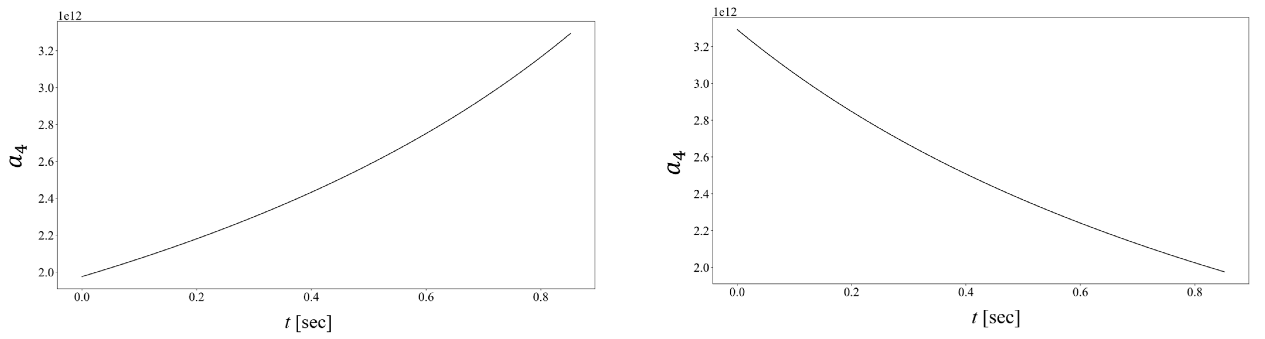
The disadvantage of the Laguerre algorithm is that small changes in the coefficients
of the characteristic polynomial
may lead to large variations about the correct values of the roots.
Figure 2 shows how these coefficients change as the eigenvalue problem for the pylon with the attached mass is solved every time step
, by retaining
eigenvalues. This leads to a
system of equations, which is the minimum size for reliable root recovery. More specifically, the left column in
Figure 2 is for the decreasing mass rate and the right column is for the increasing mass rate.
3.3. The QR Method
The QR method [
26,
27] transforms a square matrix [
D] into the product of an orthogonal matrix [
Q] (for which its transpose is the same as its inverse, i.e.,
) times an upper triangular matrix
, such that
. In order to compute the eigenvalues of
, one begins by setting an initial matrix
and performing the following iteration cycle:
After a number of iterations, matrix
converges to a lower triangular form:
The eigenvalues of the original matrix system are now recovered in closed form for each of the
submatrices appearing along the diagonal. These are complex conjugate pairs and are given by
for the
pair, where
and
are the trace and determinant of the submatrix. As a convergence criterion one may define that the absolute value of both the trace and the determinant of any
submatrix coming from the last
) iteration
is within
from the corresponding one computed from the immediately previous iteration
.
3.4. The Householder Algorithm
In general, there are three basic methods for producing the QR factorization, namely the (a) Householder, (b) Givens, and (c) Gram–Schmidt. The choice of the particular method depends on the form of the original matrix
(e.g., sparse versus fully populated) [
28]. Here we employ the Householder method, which is an algorithm requiring as input vector
plus component
and producing as output matrix
, so that the new vector
will have the remaining
components equal to zero.
Table 6 below gives the coded form of the Householder algorithm.
3.5. The QR-Householder Method
The flow of iterations begins by factorization using the Householder algorithm by starting as input vector
the first column of matrix
and receiving as output matrix
with the
elements of the first column of the matrix product
equal to zero. In our case, for the
matrix
we have
The next step produces matrix
with zero
elements of the second column of
, followed by a third step that results in an upper triangular matrix:
Arranging terms gives
, so that
, keeping in mind that all
matrices are orthogonal and symmetric. The programmed structure of this method is given in
Table 7 below.
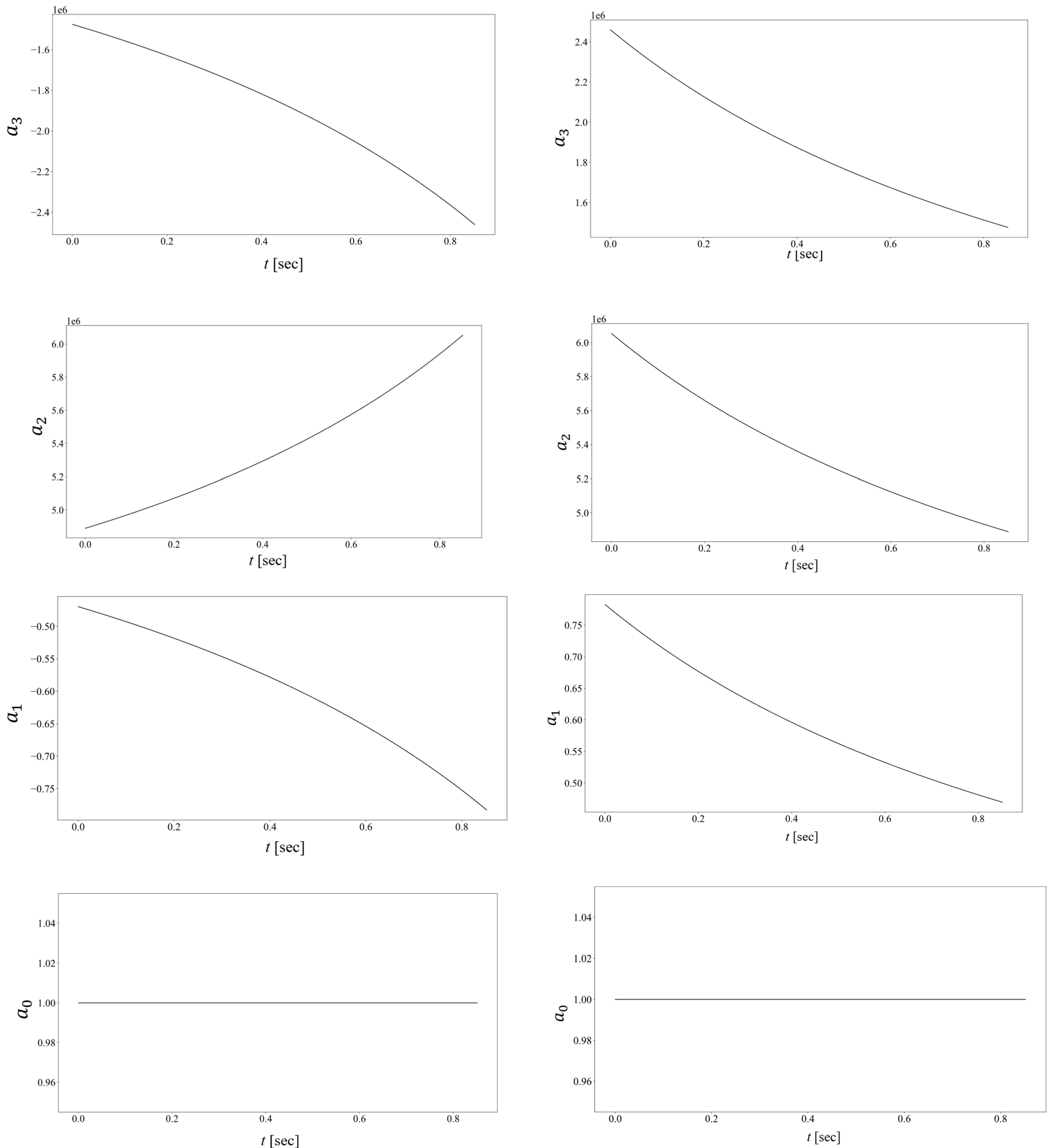
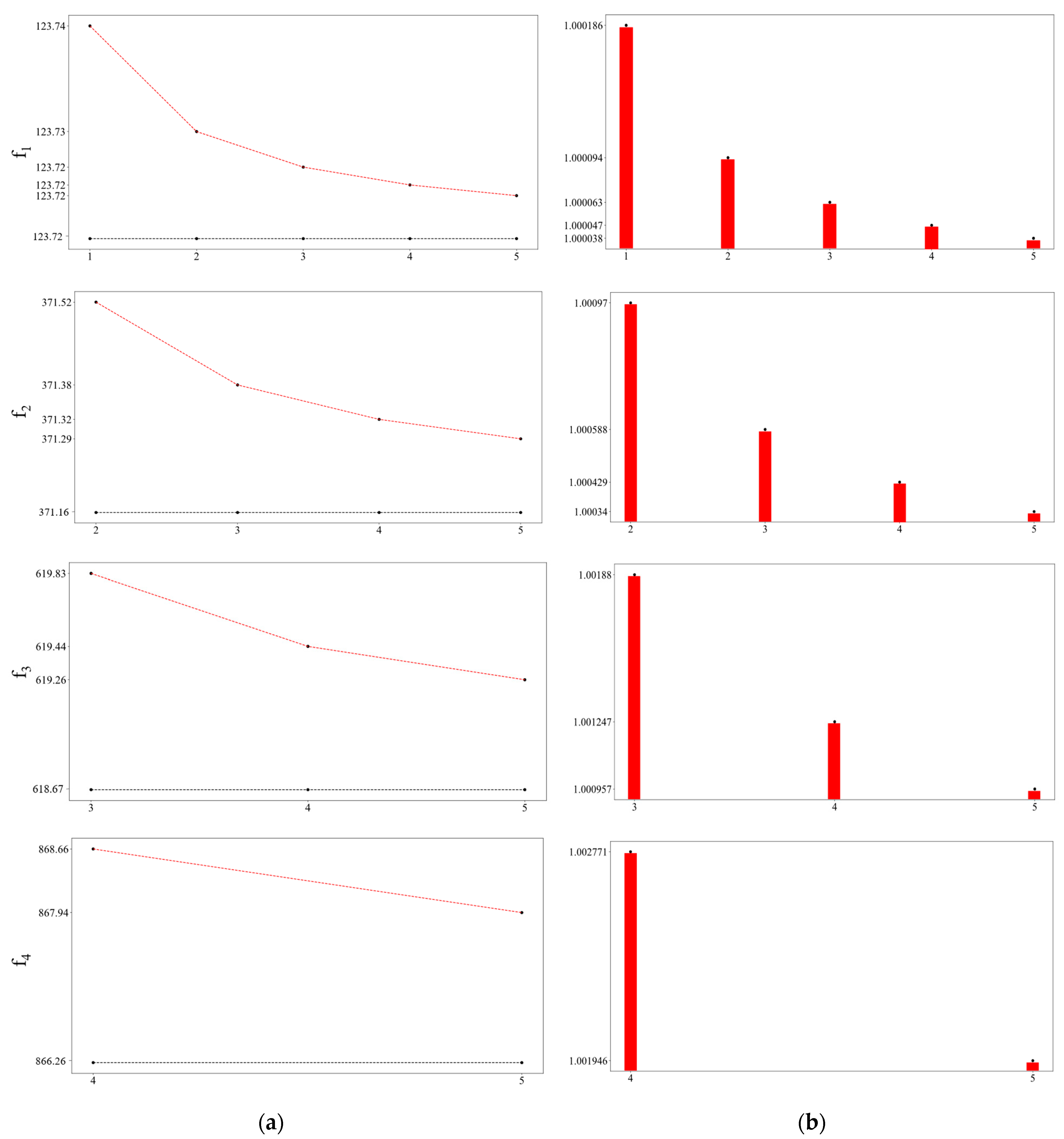
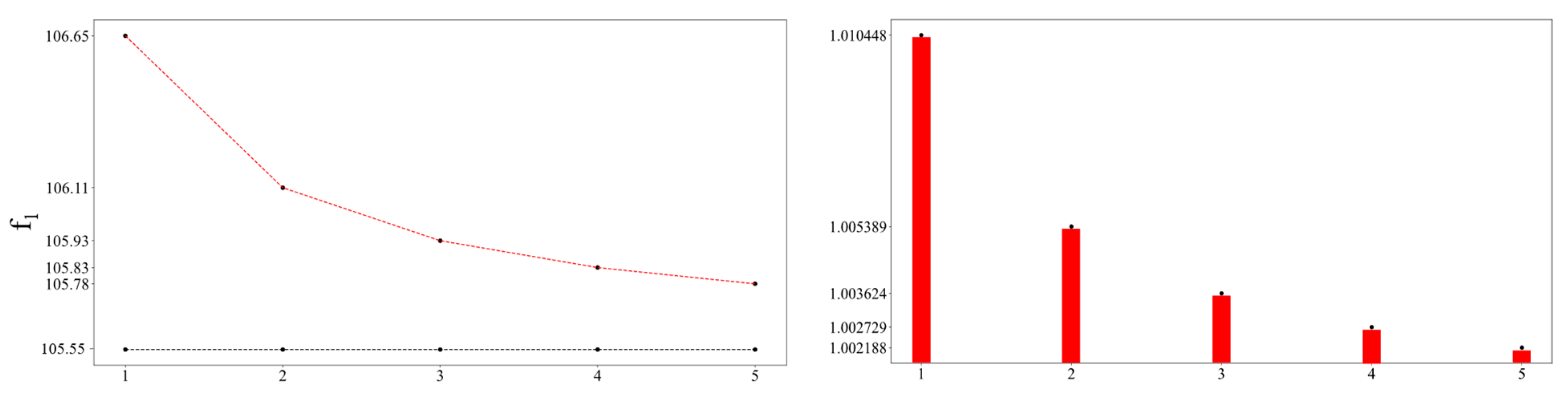
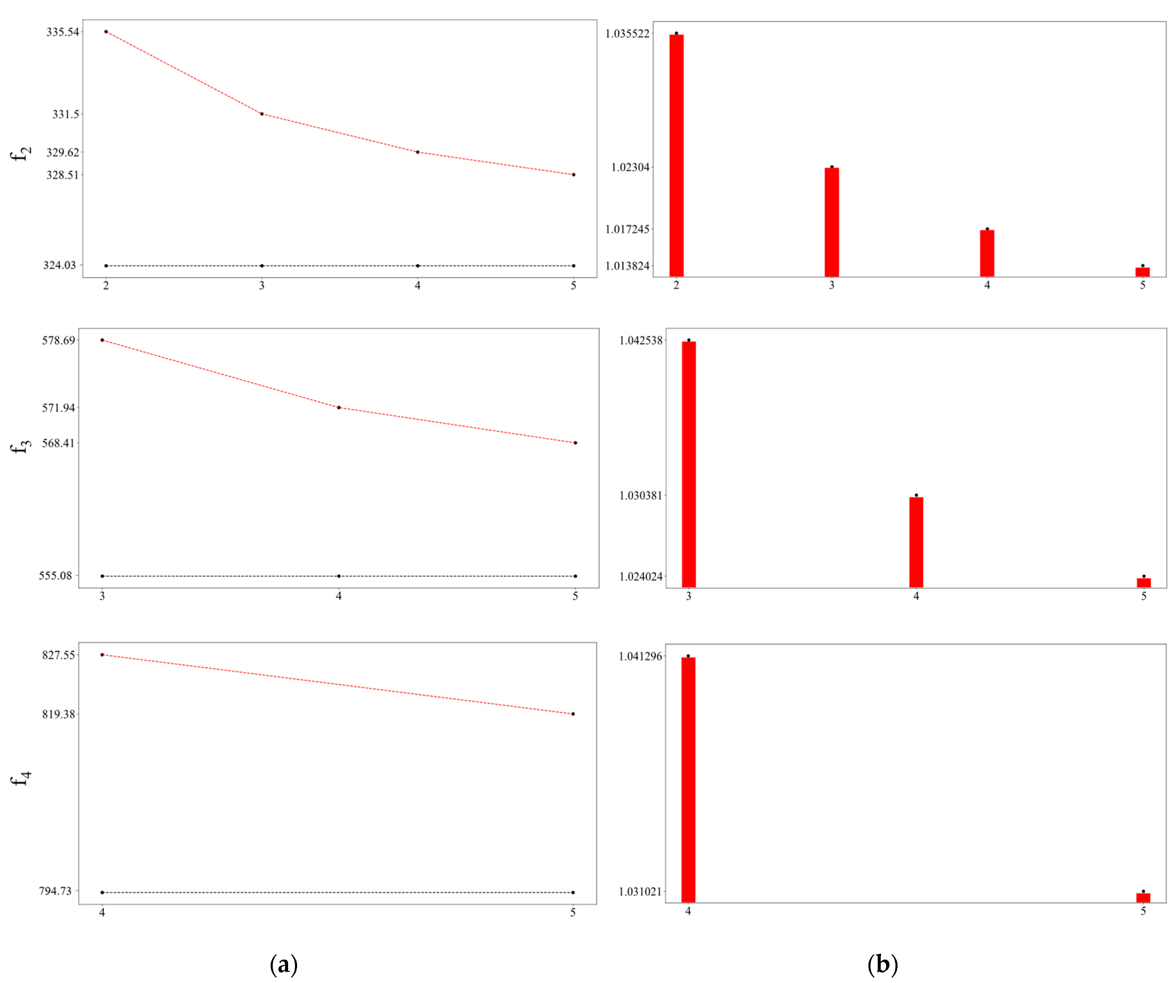
In order to determine the convergence rate of the solution of Equation (1) with the Dirac delta distribution formulation, both Laguerre and Householder-QR algorithms are tested as the size of the system matrix increases. Specifically, the ratio
, is examined, where
is the
eigenfrequency recovered by either algorithm for a system matrix of size
with
is the exact value. Thus, the left column in
Figure 3 plots the values of the first four eigenfrequencies recovered by the aforementioned algorithms (in red color), concurrently with the analytical solution (in black color) for a nearly zero mass ratio of
. At the same time, the left column in
Figure 3 plots the rate of convergence as the number
increases. Similarly,
Figure 4 plots the same information, but for a substantial mass ratio of
. In both cases, the rate of convergence is satisfactory and after
N = 5 terms, the error is negligible. Note that both algorithms give the same ratio for size
, past which the Laguerre is no longer accurate and only the Householder-QR algorithm is used.
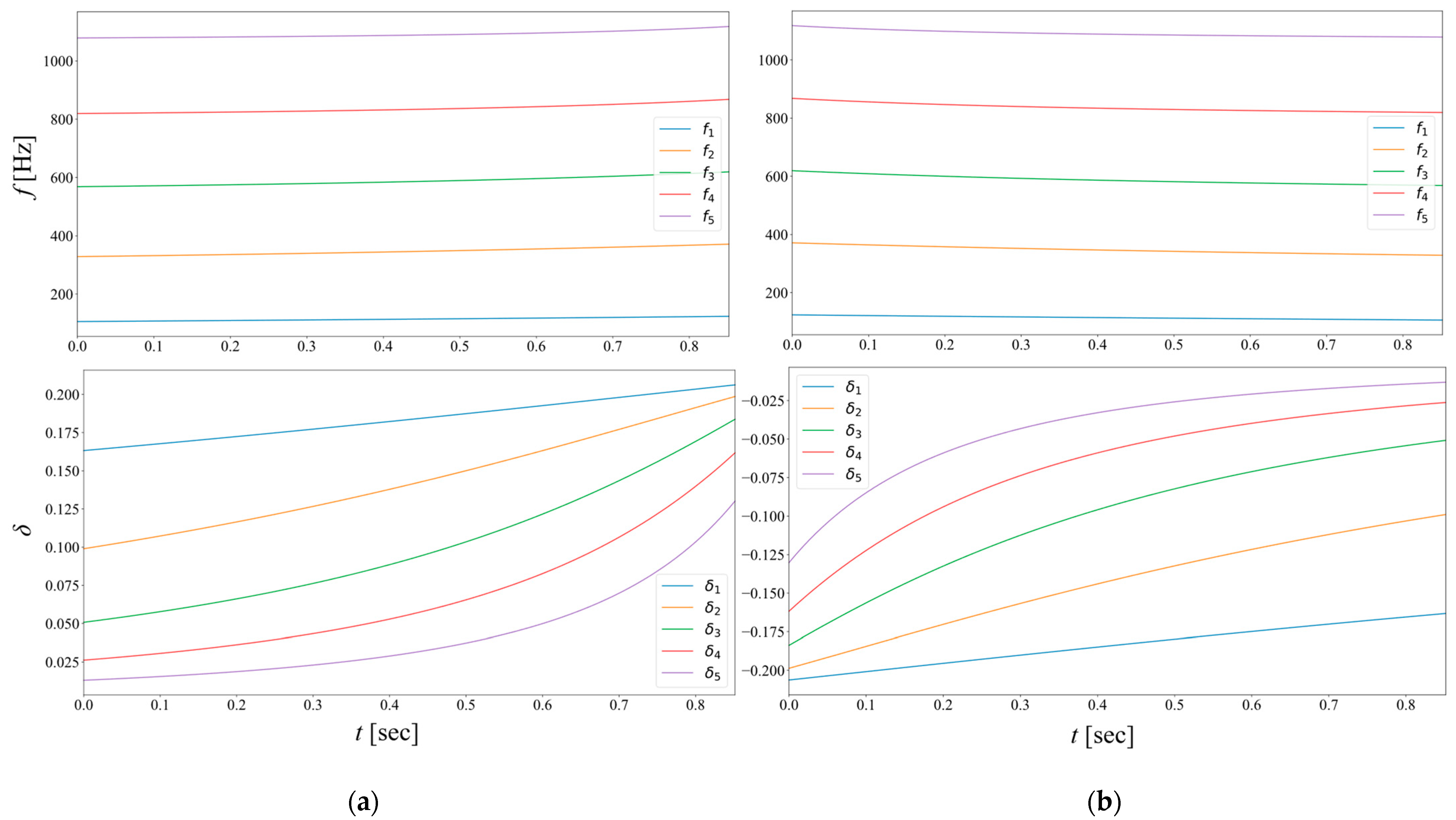
3.6. Time Evolution of the Pylon Eigenvalues
When working with
terms in Equation (5), ten roots
are recovered by the QR Householder method for the eigenvalues, which appear as complex conjugate pairs. These are now plotted in
Figure 5 as
(see Equation (13)) and the real part
(see Equation (12)) for every time step
starting from time zero to time
T, past which the flow has stopped and we either have a stand-alone pylon or a pylon with a fixed top mass
. We clearly observe in
Figure 5 the evolution of the eigenvalues for longitudinal vibrations of the pylon as the mass of the water tank changes over time. As expected, this system becomes stiffer as its mass decreases (
Figure 5a) and becomes more flexible as its mass increases (
Figure 5b). In either case, the eigenfrequencies converge to their expected values when the system is stationary.
4. Derivation of Spectograms
For SHM purposes, it is necessary to trace the evolution of the eigenvalues of the pylon as its attached mass varies with time from tracing the transient displacement
at a given station
. In reference to the pylon described in
Section 2, the dynamic characteristics of the combined pylon-attached mass system vary with time and the resulting transient response is characterized from a stochastic viewpoint as non-stationary. This requires subjecting the transient signal to a series of continuous transformations to the frequency domain by implementing the short time Fourier transformation (STFT). For sufficiently small-time steps, the signal recorded within a given time interval can be considered as stationary. To this purpose, we employ the Fourier transform [
22] in the following form:
In the above,
is a Fourier transform of the pylon displacement at
, see Equation (5), and is known as a spectrogram. Moreover,
is the frequency (in
) and function
is the Hanning window within a time interval
:
The width of the Hanning window is and should cover at least one cycle of vibration. Fixing the window’s width, as well as the placement of two consecutive windows, is a trial-and-error procedure for achieving optimal results.
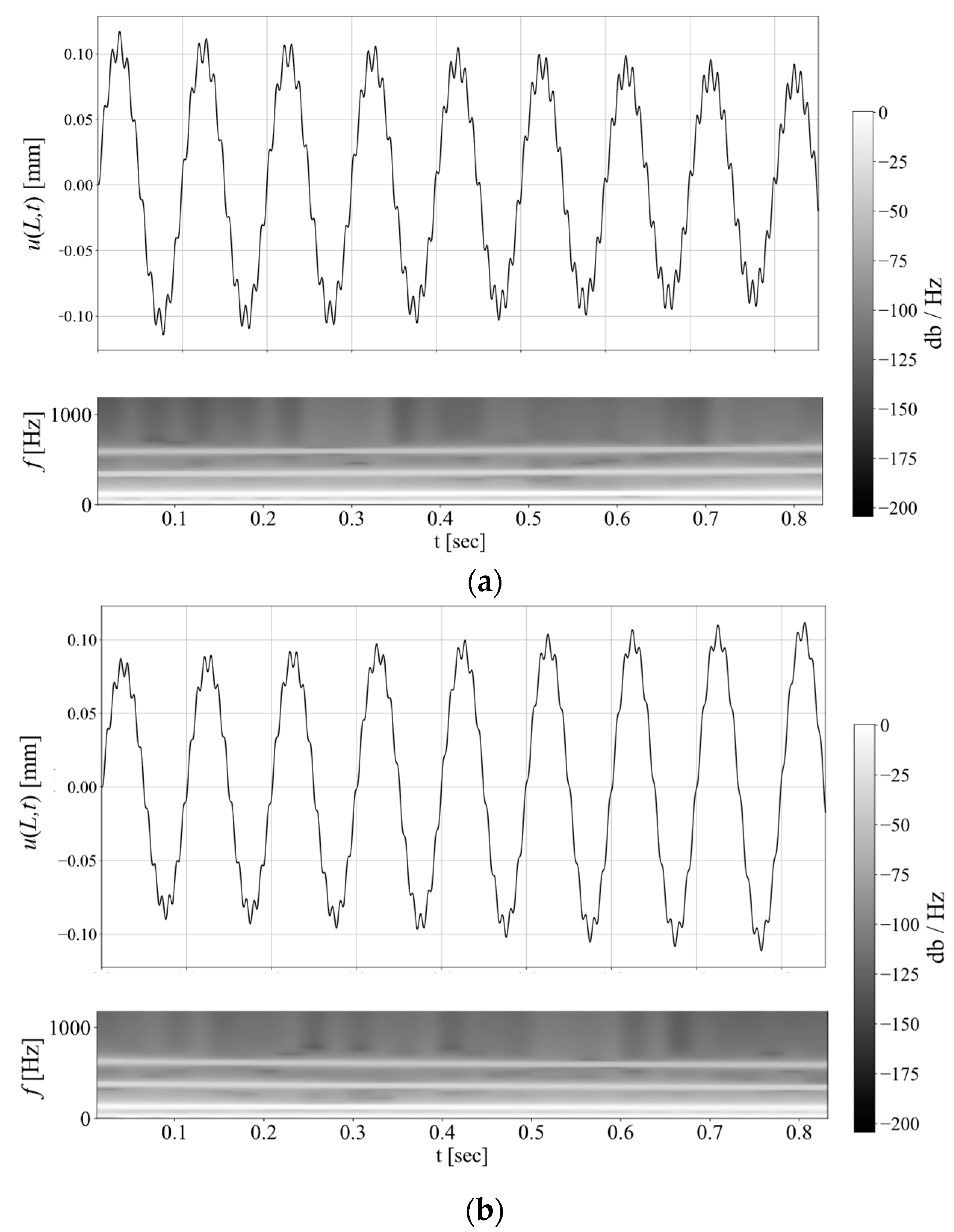
The derivation of a spectrogram is now given for both cases where the mass attachment on the pylon is either full of a liquid that is allowed to drain, or empty and allowed to fill. At first,
Figure 6 plots the transient response at the top of the pylon following a modal analysis based on the results of the eigenvalue extraction problem. Note that when alternative numerical methods such as the Runge–Kutta method are used for computing the transient displacements, then the time evolution of the eigenvalues cannot be recovered directly, but require additional processing by various transformation techniques. The input is a time harmonic ground motion with an excitation frequency of
. As the attached mass decreases with time, the structural system becomes stiffer and the response of the pylon slowly decreases by about 18% at the end of the time interval of about 0.85 s required to completely remove the mass, see
Figure 6a. At the same time, the corresponding spectrogram, which reproduces the analytically computed time evolution of the combined system eigenfrequencies that was previously obtained, shows a 30% change as the system becomes stiffer due to the decreasing top mass. Finally, the white line at the bottom of the plot corresponds to the forcing frequency of
. The exact opposite behavior is shown in
Figure 6b, with the response increasing and the eigenfrequencies dropping as the system becomes more flexible with time.
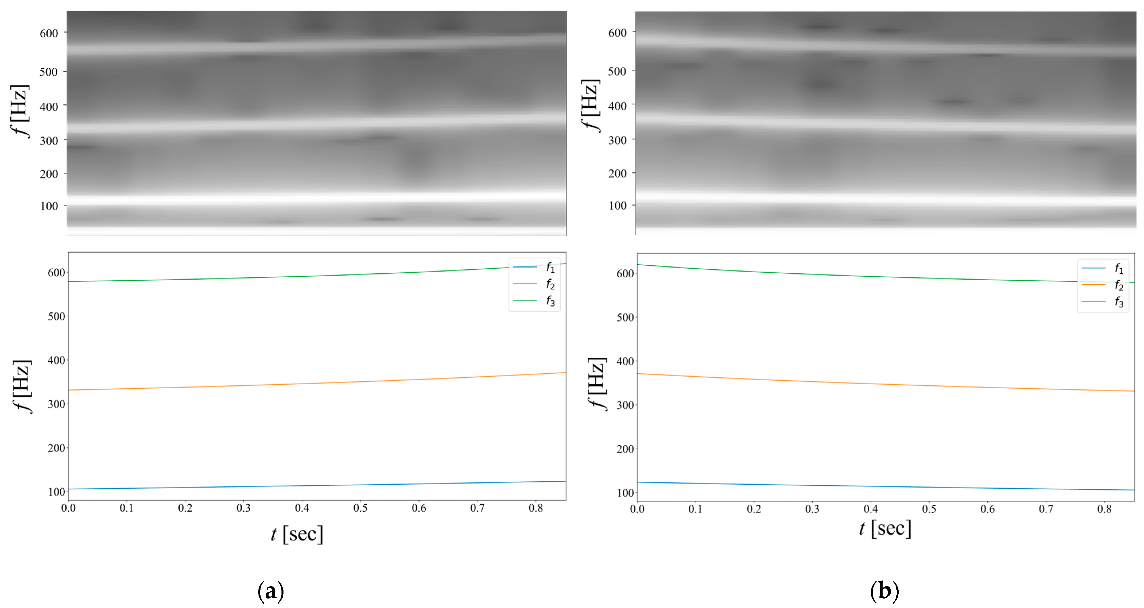
Comparison of Results
In this section, we compare the results for the eigenvalues of the pylon with a time variable mass, as computed by the iterative methods of solution, see
Section 3, and also indirectly from the spectograms given above. Note that these spectograms were derived from a numerical solution of the equations of motion using the Runge–Kutta method that yielded the displacement function, to which the short-term Fourier transform was applied. The comparison is limited to three eigenvalues, because it becomes exceedingly difficult to derive higher-order eigenvalues from the results given by the Runge–Kutta method.
Figure 7 depicts the results of this comparison study, which shows good agreement between the pylon eigenvalues recovered from these two basic categories of solving transient problems.
5. Discussion and Conclusions
This work investigates the applicability of iterative eigenvalue extraction algorithms for the purpose of structural identification. More specifically, the application example is a flexible, metallic cantilevered pylon with a time-dependent mass attachment. This specific attachment renders the eigenvalue problem time-dependent for the time duration of the action of the applied loads. Once the transient motion at a given station on the pylon is synthesized by modal analysis, the application of the short-time Fourier transform yields a clear picture of the manner in which the eigenvalues of the combined pylon-mass structural system vary during the action of ground-induced motions.
Focusing on the eigenvalue analysis of the combined pylon-mass system, at first the coefficients of the polynomial resulting from setting the determinant of the first-order matrix system formulation equal to zero are recovered using the Leverrier–Faddeev algorithm. This is a recursive method for calculating the coefficients of the characteristic polynomial of a square matrix [
13]. However, these coefficients show large differences in their absolute values rendering any subsequent method for extracting eigenvalues potentially unstable. Therefore, the eigenvalue extraction is first performed by the Laguerre method, which is the complex number variant of the conventional Newton–Raphson method used for real root extraction [
14,
15]. For the Laguerre method, an additional complication is computing the correct initial values at the beginning of each time step, which are the final values of the immediately previous time step. Next, the QR method [
16] is implemented in conjunction with the Householder algorithm, which is the best option in terms of both accuracy and efficiency, while all limiting cases are correctly reproduced when the attached mass attains a fixed value. In general, it is estimated that three eigenvalues are necessary for any subsequent modal analysis when the attached point mass is at a boundary, which in our case is the top of the pylon. If the mass is attached at an intermediate station on the pylon, then two eigenvalues are sufficient, which implies one can use the Laguerre method as well.
At first, an analytical solution for the axial motion of the pylon modeled as a distributed mass system is derived, with the formulation augmented to handle an attached, time-dependent mass attachment at the top which is heavy and cannot be viewed as a secondary system. The solution is obtained by modal analysis following the eigenvalue extraction. What complicates the solution is the fact that the mass is time-dependent, i.e., may either increase or decrease during the time interval the external forces are active. This requires a second-tier solution of a time-dependent eigenvalue problem cast as a system of first order differential equations with non-constant coefficients. Next, the eigenvalues are plotted against the time duration of the increasing/decreasing fluid flow from a container at the top of the pylon. The stiffening/softening of the combined fluid mass-pylon system is manifested as a function of fluid decrease/increase in the container. Then, the time histories at any station on the pylon for ground-induced motions can be computed by modal analysis. Finally, if structural identification is the goal, then the aforementioned time histories can be used as raw date, followed by application of the FT with Hanning windows sequentially places across the time axis.
In general, the methodology developed herein is applicable to other types of structural systems with transient mass attachments and to general types of dynamic loads, including the case of a moving mass. A common case is the fixed, lumped mass at the top, which may also act as a secondary system in the case of light-weight appendages. It is also possible to augment the present formulation to model a compliant foundation by introducing equivalent soil springs at the base of the pylon, and finally to treat beams with a non-uniform cross-section. One field of application of this work is SHM for pylons used in electrified rail lines, where high frequency ground vibrations are induced in the vertical direction due to the passage of fast trains. In this case the presence of a time-variable lumped mass at the top of the pylon may either be detrimental or beneficial, depending on the frequency content of the external excitation and on the rate by which this mass increases or decreases.


