

On a Hypothetical Model with Second Kind Chebyshev’s Polynomial–Correction: Type of Limit Cycles, Simulations, and Possible Applications


Abstract
1. Introduction
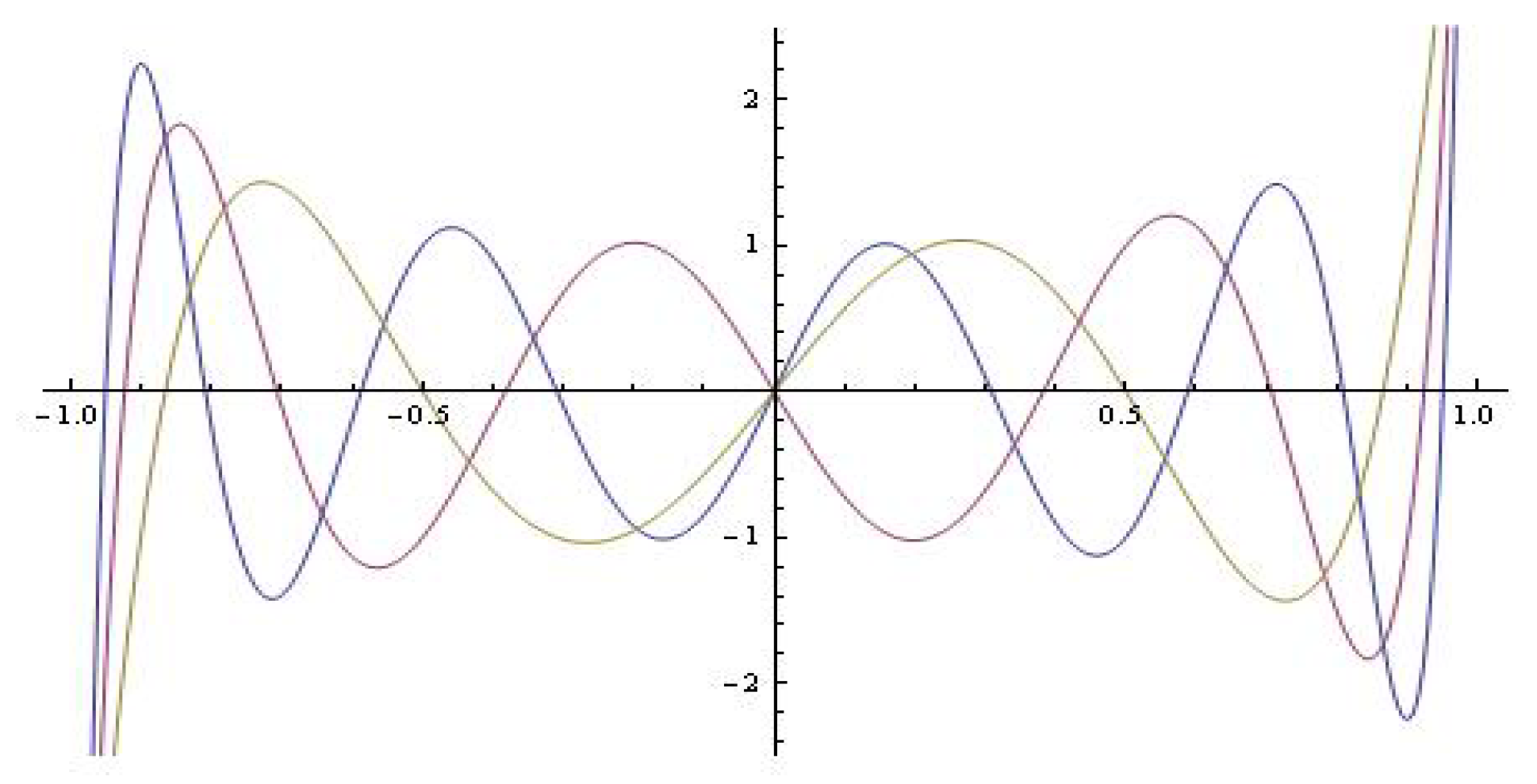
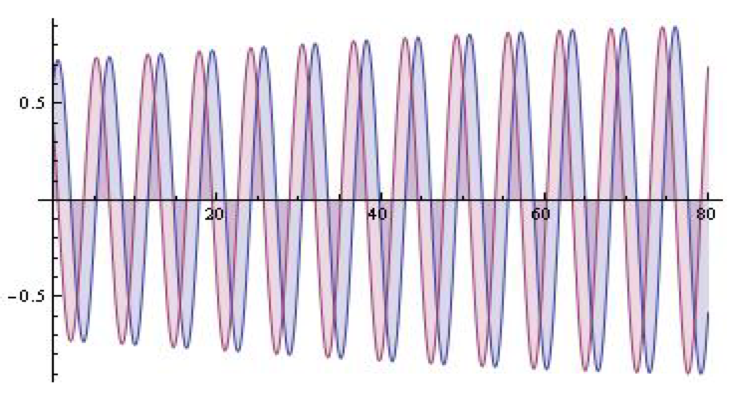
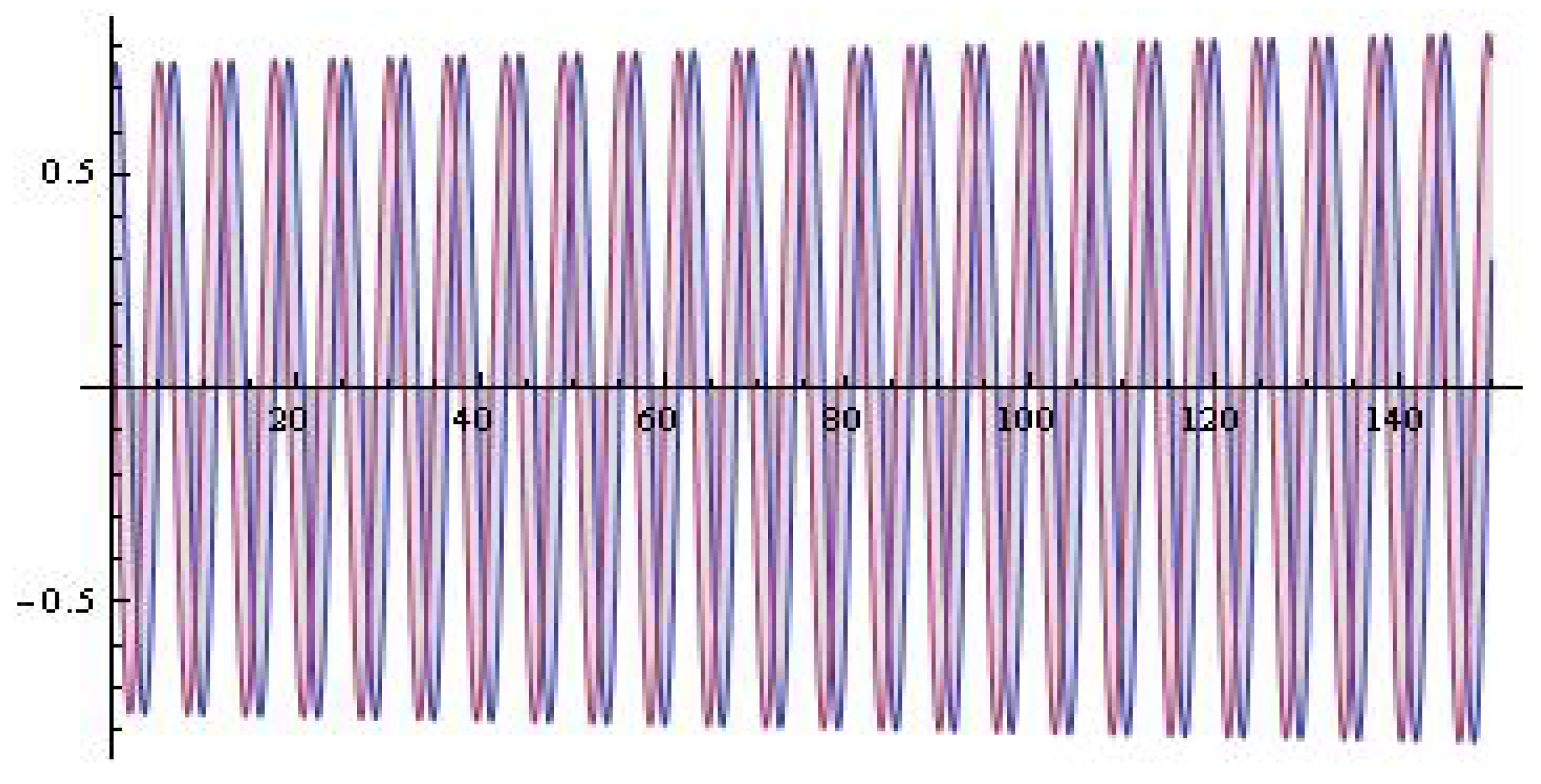
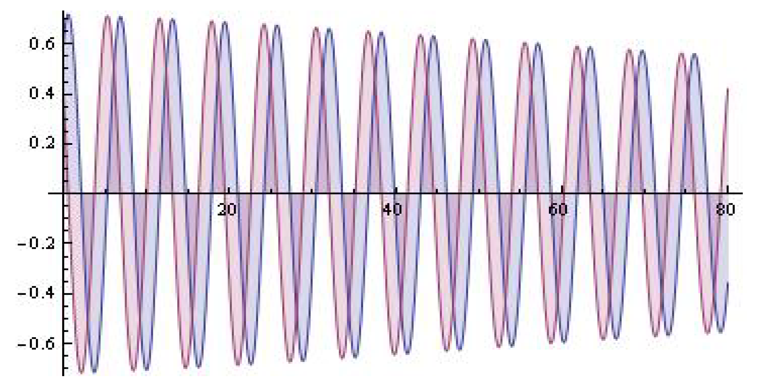
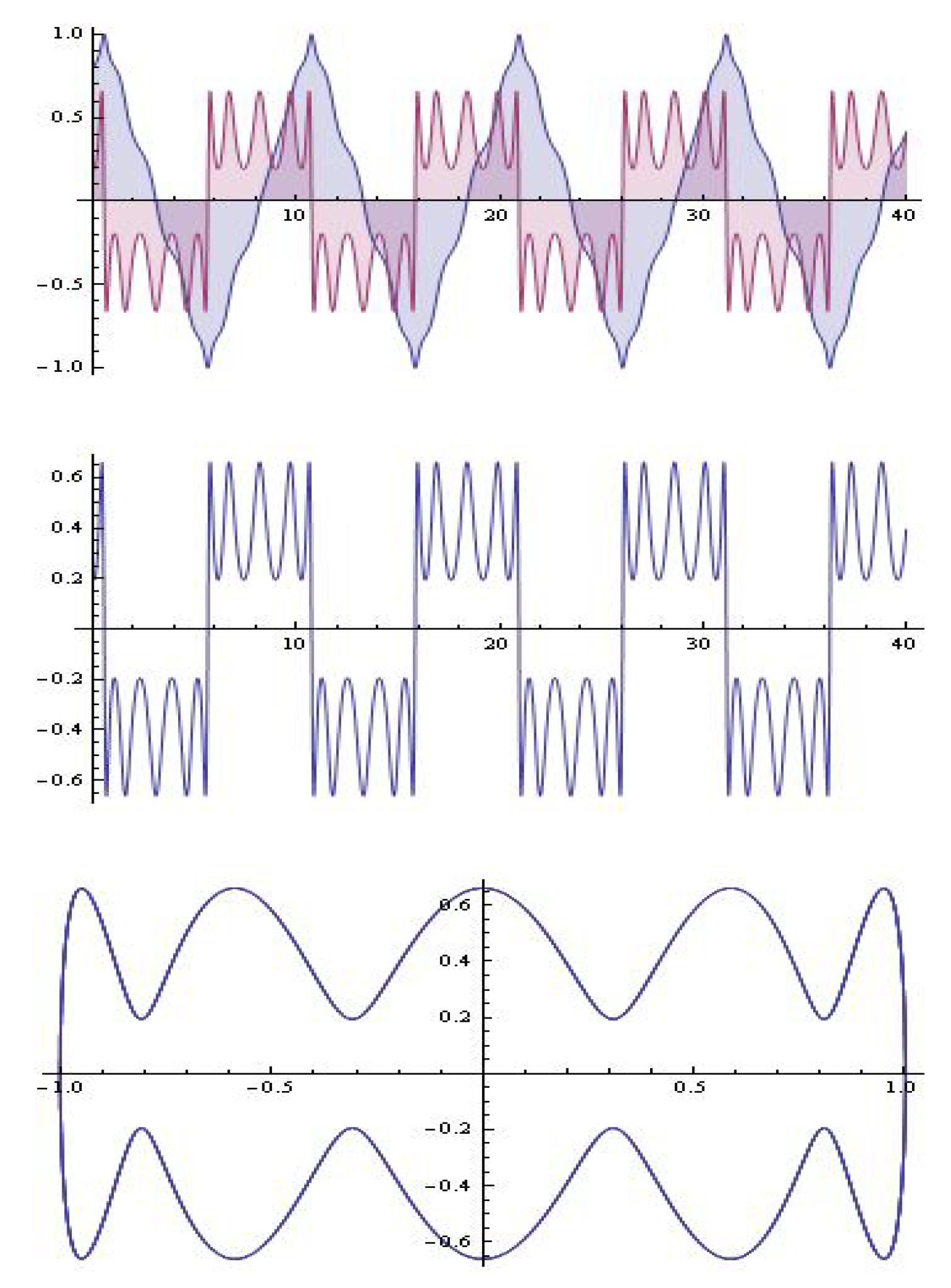
2. Main Results–Simulations
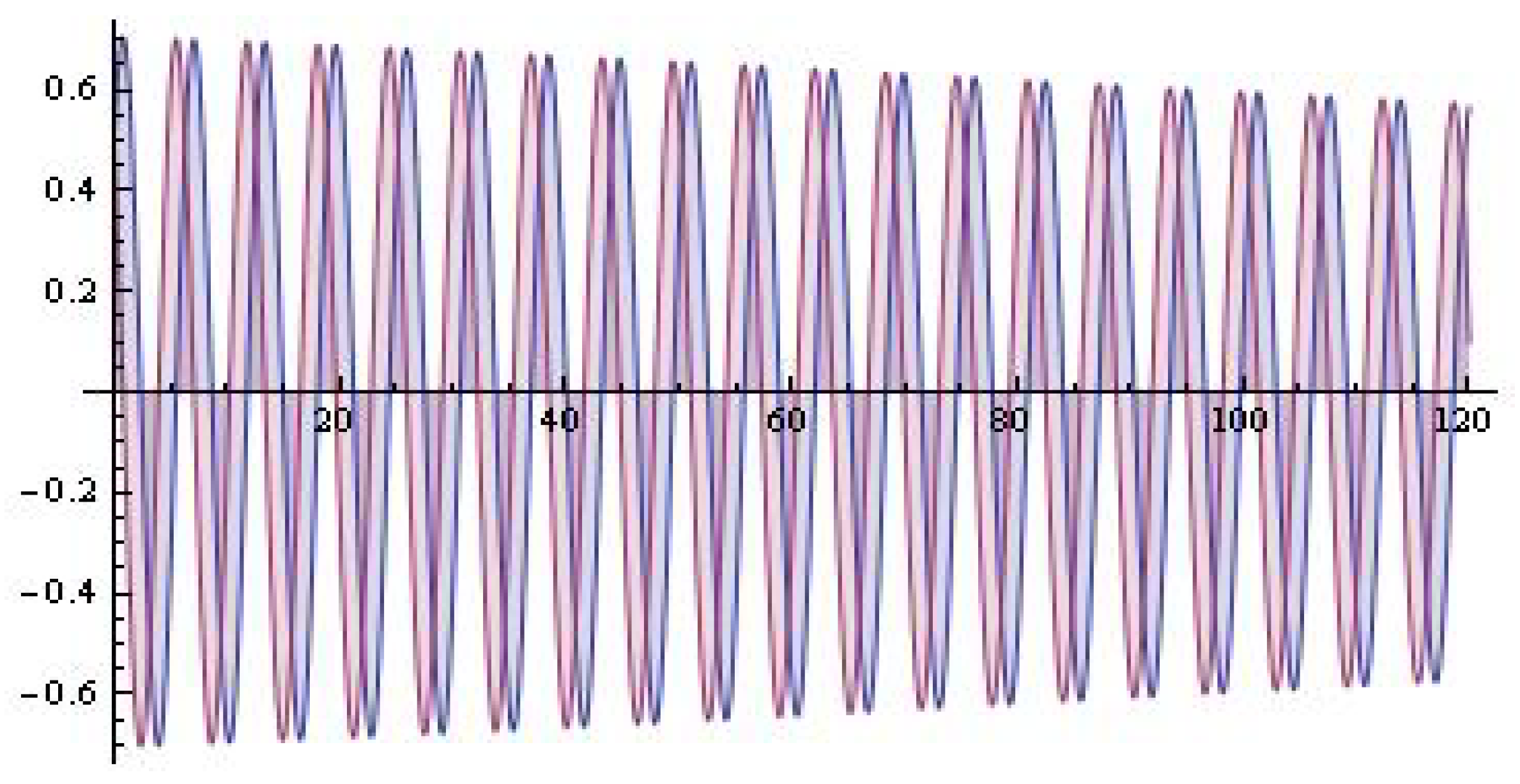
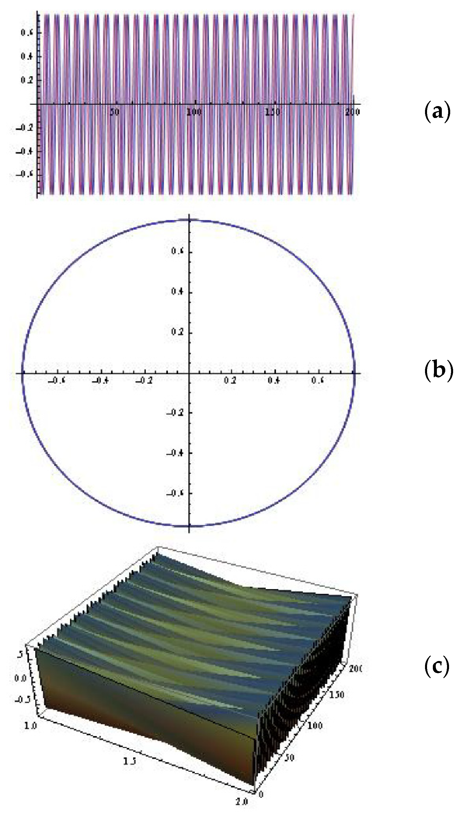
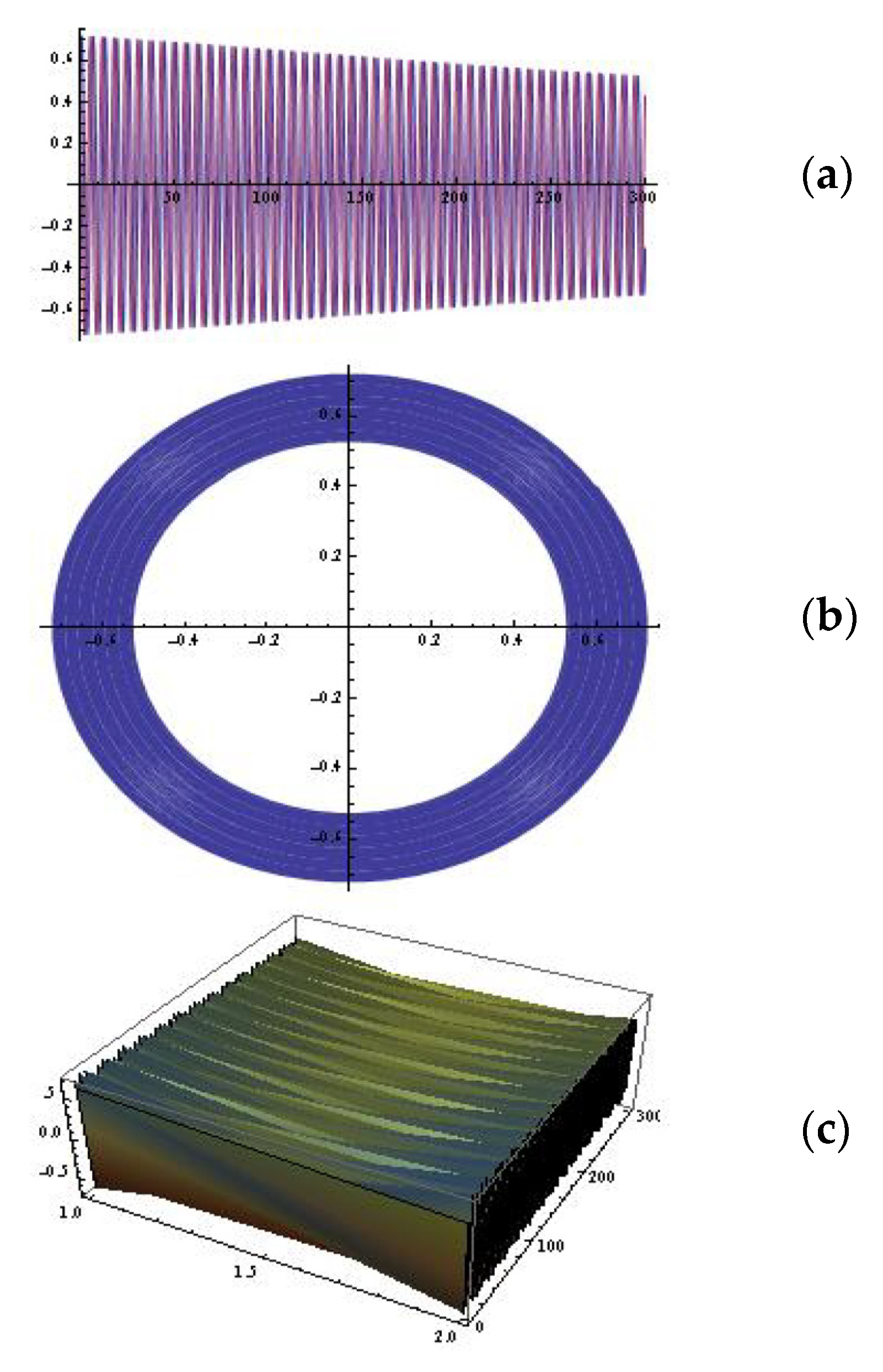
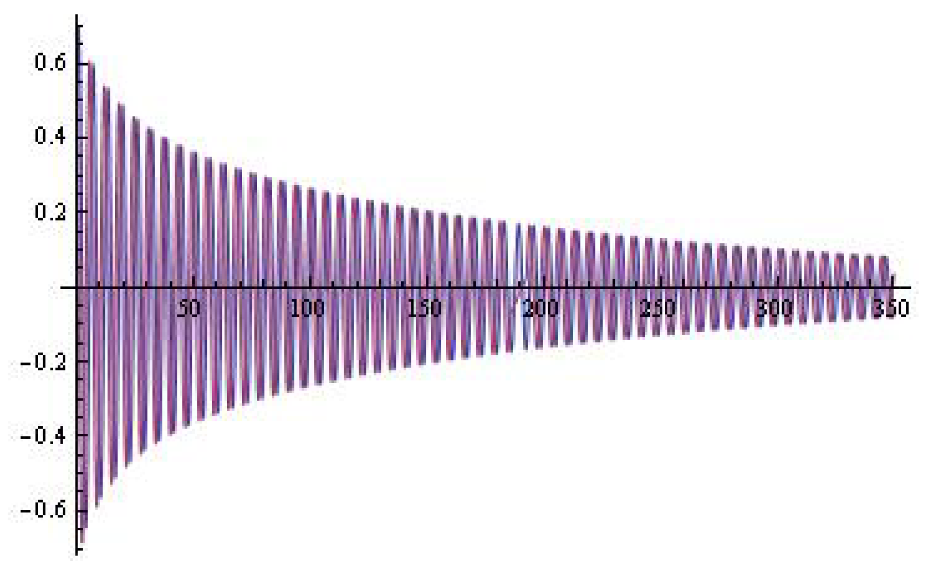
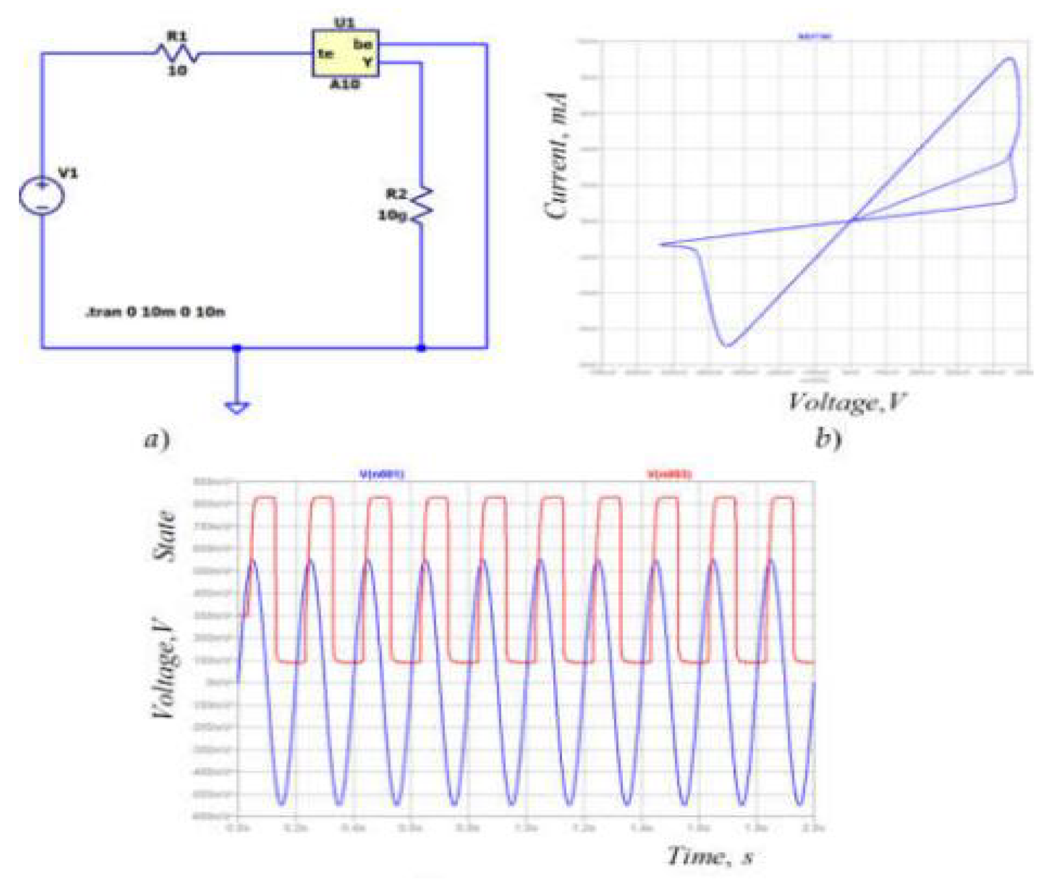
2.1. Extended Lienard-Type Planar System
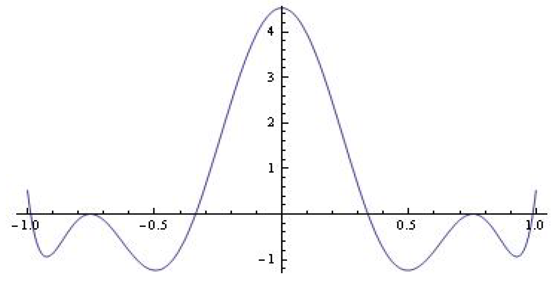
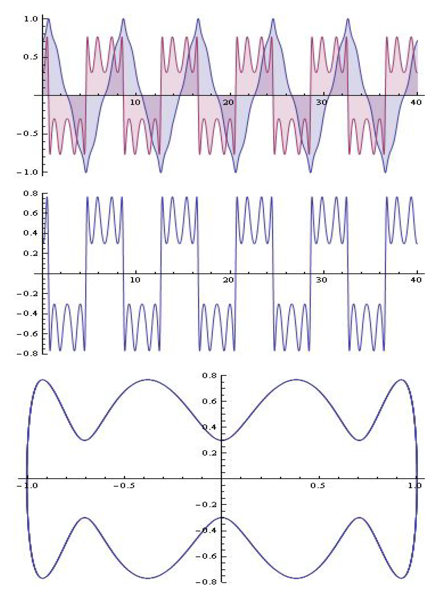
2.2. The New Model in the Light of Melnikov’s Considerations
2.3. Related Problems and Possible Applications
3. Concluding Remarks
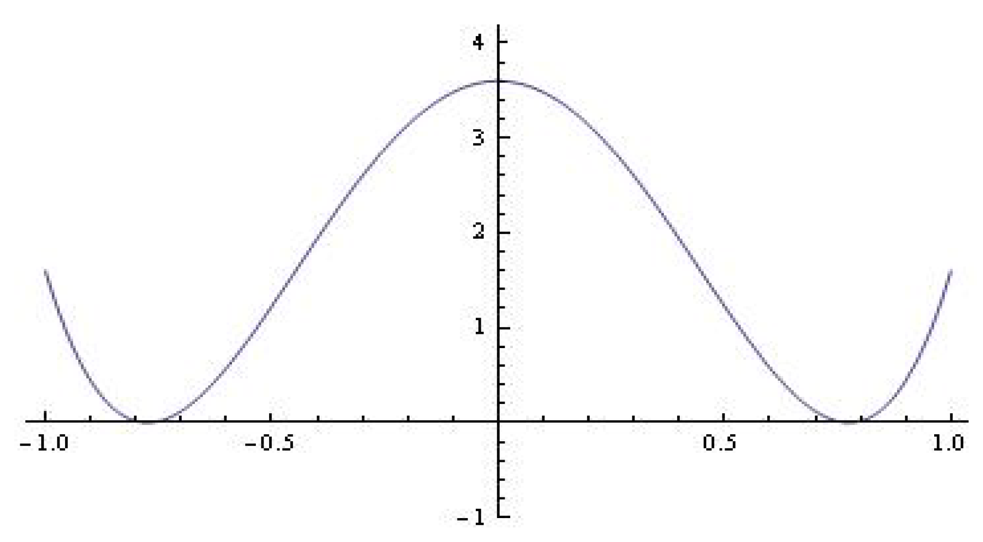
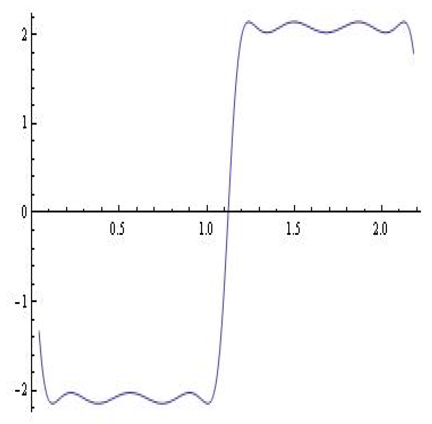
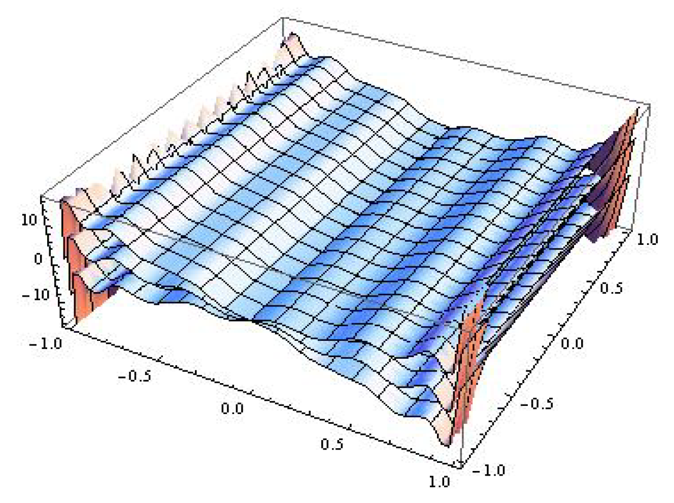
3.1. Numerical Issues Connected to the Investigation of the Roots of the Melnikov Polynomial
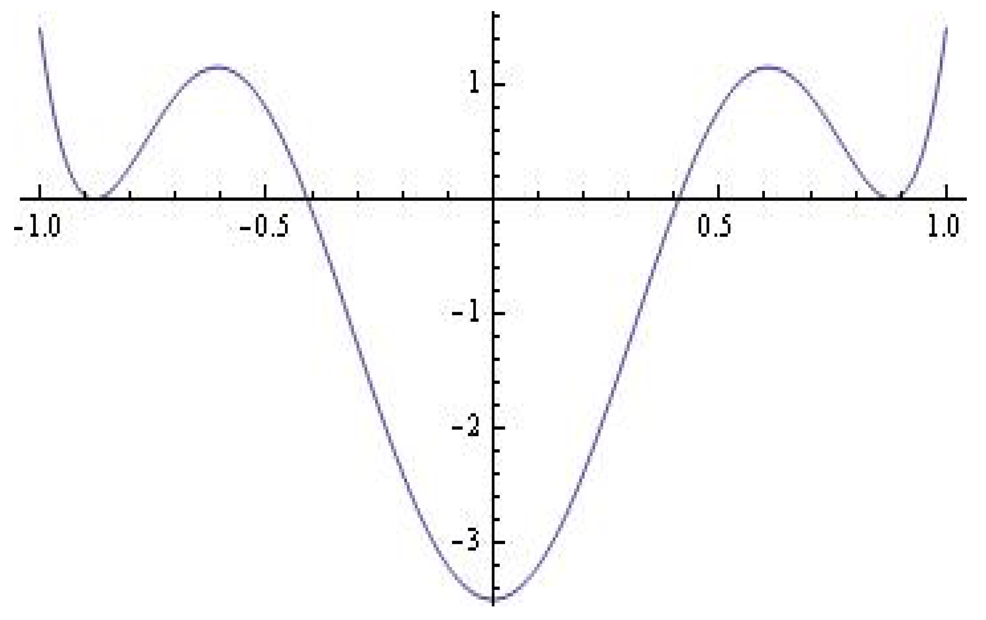
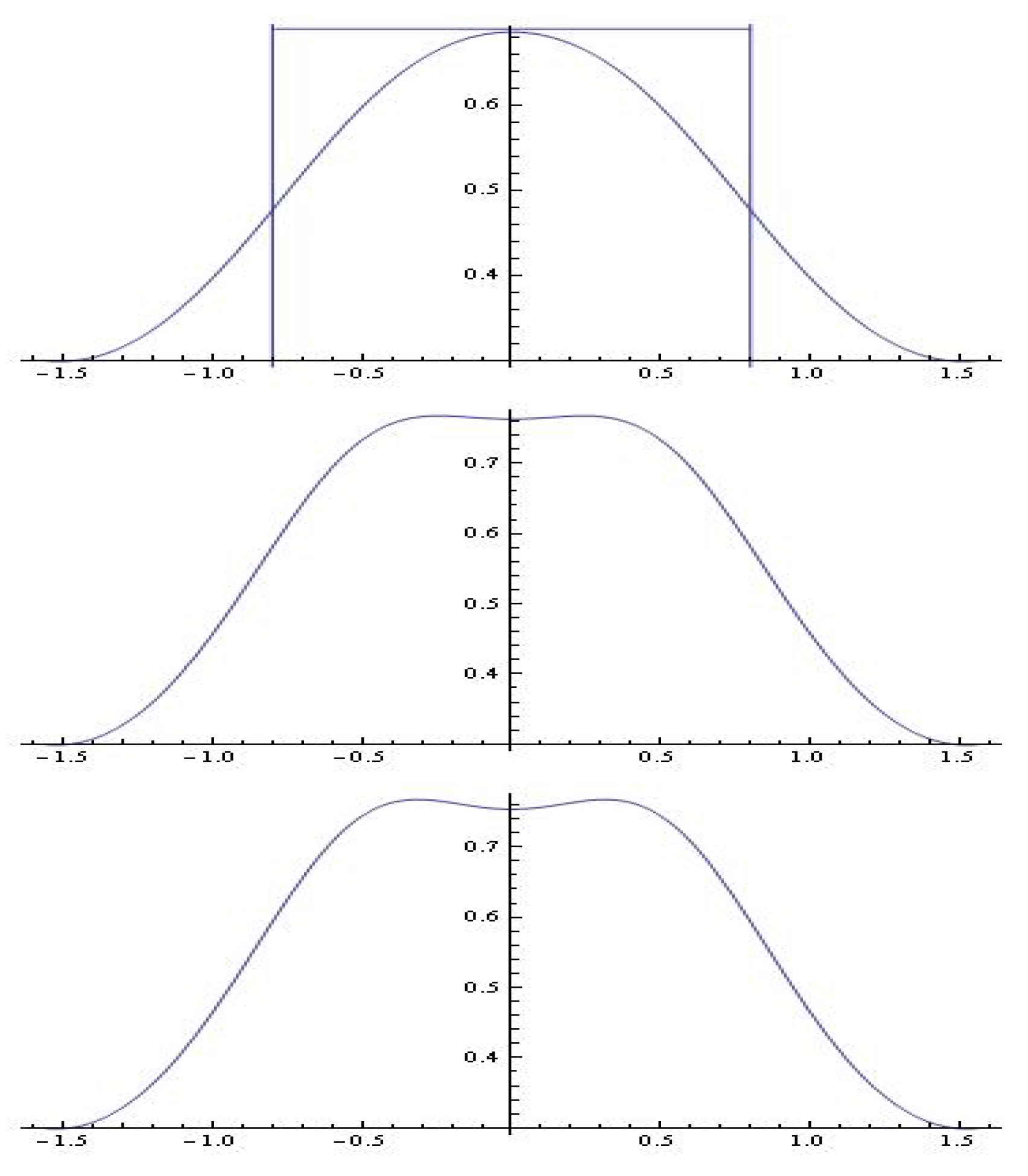
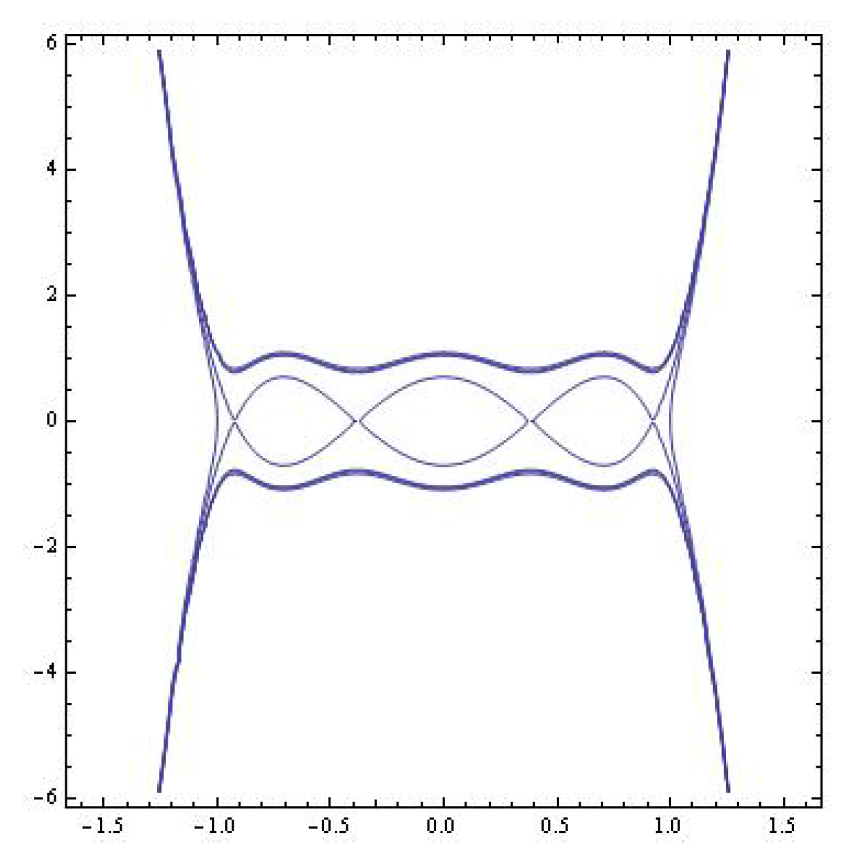
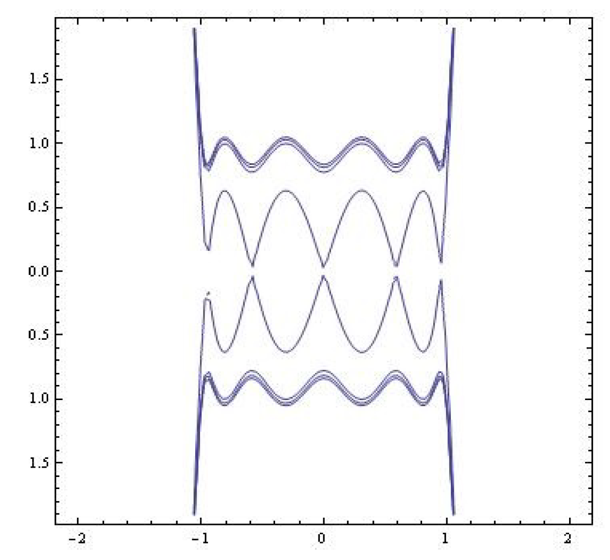
3.2. The Level Curves
Author Contributions
Funding
Institutional Review Board Statement
Informed Consent Statement
Data Availability Statement
Acknowledgments
Conflicts of Interest
References
- Hilbert, D. Mathematical problems (M.Newton Transl.). Bull. Am. Math. Soc. 1901, 8, 437–479. [Google Scholar] [CrossRef]
- Melnikov, V.K. On the stability of a center for time–periodic perturbation. Trudy Moskovskogo Matematicheskogo Obshchestva 1963, 12, 3–52. [Google Scholar]
- Lienard, A. Etude des oscillations entretenues. Revue Generale de e’Electricite 1828, 23, 901–912, 946–954. [Google Scholar]
- Blows, T.; Perko, L. Bifurcation of Limit Cycles from Centers and Separatrix Cycles of Planar Analytic Systems. SIAM Rev. 1994, 36, 341–376. [Google Scholar] [CrossRef]
- Perko, L. Differential Equations and Dynamical Systems; Springer: New York, NY, USA, 1991. [Google Scholar]
- Kyurkchiev, N.; Andreev, A. Approximation and Antenna and Filters Synthesis. Some Moduli in Programming Environment Mathematica; LAP LAMBERT Academic Publishing: Saarbrucken, Germany, 2014; 150p, ISBN 978-3-659-53322-8. [Google Scholar]
- Kyurkchiev, V.; Kyurkchiev, N. On an extended relaxation oscillator model: Number of limit cycles, simulations. I. Commun. Appl. Anal. 2022, 26, 19–42. [Google Scholar]
- Tadmor, E.; Tanner, J. Adaptive filters for piecewise smooth spectral data. IMA J. Numer. Alg. 2005, 25, 535–547. [Google Scholar] [CrossRef]
- Tanner, J. Optimal filter and mollifier for piecewise smooth spectral data. Math. Comput. 2006, 75, 767–790. [Google Scholar] [CrossRef]
- Kyurkchiev, N. Some Intrinsic Properties of Tadmor-Tanner Functions: Related Problems and Possible Applications. Mathematics 2020, 8, 1963. [Google Scholar] [CrossRef]
- Mladenov, V. A unified and open LTSPICE memristor model library. Electronics 2021, 10, 1594. [Google Scholar] [CrossRef]
- Mladenov, V.; Kirilov, S. A Neural Synapse Based on Ta2O5 Memristor. In Proceedings of the 2021 17th International Workshop on Cellular Nanoscale Networks and their Applications (CNNA), Catania, Italy, 29–30 September 2021. [Google Scholar] [CrossRef]
- Mladenov, V.; Kirilov, S. A Simplified Tantalum Oxide Memristor Model, Parameters Estimation and Application in Memory Crossbars. Technologies 2022, 10, 6. [Google Scholar] [CrossRef]
- Mladenov, V.M.; Zaykov, I.D.; Kirilov, S.M. Application of a Nonlinear Drift Memristor Model in Analogue Reconfigurable Devices. In Proceedings of the 2022 26th International Conference Electronics, Palanga, Lithuania, 13–15 June 2022; pp. 1–6. [Google Scholar]
- Mladenov, V. Advanced Memristor Modeling–Memristor Circuits and Networks; MDPI: Basel, Switzerland, 2019. [Google Scholar]
- Mladenov, V. Analysis and Simulations of Hybrid Memory Scheme Based on Memristors. Electronics 2018, 7, 289. [Google Scholar] [CrossRef]
- Kyurkchiev, V.; Iliev, A.; Rahnev, A.; Kyurkchiev, N. A technique for simulating the dynamics of some extended relaxation oscillator models. II. Commun. Appl. Anal. 2022, 26, 43–59. [Google Scholar]
- Kyurkchiev, V.; Iliev, A.; Rahnev, A.; Kyurkchiev, N. Another extended polynomial Lienard systems: Simulations and applications. III. Int. Electron. J. Pure Appl. Math. 2022, 16, 55–65. [Google Scholar]
- Kyurkchiev, V.; Iliev, A.; Rahnev, A.; Kyurkchiev, N. Investigations on some polynomial Lienard-type systems: Number of limit cycles, simulations. Int. J. Differ. Equ. Appl. 2022, 21, 117–126. [Google Scholar]
- Kyurkchiev, V.; Kyurkchiev, N.; Iliev, A.; Rahnev, A. On Some Extended Oscillator Models: A Technique for Simulating and Studying Their Dynamics; Plovdiv University Press: Plovdiv, Bulgaria, 2022; ISBN 978-619-7663-13-6. [Google Scholar]
- Beltrami, E. Mathematics for Dynamic Modeling; Academic Press: Boston, MA, USA, 1987. [Google Scholar]
- Arnold, V. Geometrical Methods in the Theory of Ordinary Differential Equation; Springer: Berlin/Heidelberg, Germany, 1988. [Google Scholar]
- Zeeman, E. Catastrophe Theory. Selected Papers 1972–1977; Addison-Wesley: Reading, MA, USA, 1977. [Google Scholar]
- Kyurkchiev, N.; Andreev, A.; Popov, V. Iterative methods for the computation of all multiple roots of an algebraic polynomial. Annu. Univ. Sofia Fac. Math. Mech. 1984, 78, 178–185. [Google Scholar]
- Proinov, P.; Vasileva, M. On the convergence of high-order Ehrlich-type iterative methods for approximating all zeros of a polynomial simultaneously. J. Inequalities Appl. 2015, 2015, 336. [Google Scholar] [CrossRef]
- Proinov, P.D.; Vasileva, M.T. Local and Semilocal Convergence of Nourein’s Iterative Method for Finding All Zeros of a Polynomial Simultaneously. Symmetry 2020, 12, 1801. [Google Scholar] [CrossRef]
- Kyncheva, V.; Yotov, V.; Ivanov, S. Convergence of Newton, Halley and Chebyshev iterative methods as methods for simultaneous determination of multiple zeros. Appl. Numer. Math. 2017, 112, 146–154. [Google Scholar] [CrossRef]
- Petkovic, I.; Herceg, D. Computer methodologies for comparison of computational efficiency of simultaneous methods for finding polynomial zeros. J. Comput. Appl. Math. 2020, 368, 112513. [Google Scholar] [CrossRef]
- Kanno, S.; Kjurkchiev, N.; Yamamoto, T. On some methods for the simultaneous determination of polynomial zeros. Jpn. J. Appl. Math. 1995, 13, 267–288. [Google Scholar] [CrossRef]
- Llibre, J.; Valls, C. Global centers of the generalized polynomial Lienard differential systems. J. Differ. Equ. 2022, 330, 66–80. [Google Scholar] [CrossRef]
- Chen, H.; Lie, Z.; Zhang, R. A sufficient and necessary condition of generalized polynomial Lienard systems with global centers. arXiv 2022, arXiv:2208.06184. [Google Scholar]
- He, H.; Llibre, J.; Xiao, D. Hamiltonian polynomial differential systems with global centers in the plane. Sci. China Math. 2021, 48, 2018. [Google Scholar]
- Smale, S. Mathematical problems for the next century. Math. Intell. 1998, 20, 7–15. [Google Scholar] [CrossRef]
- Zhao, Y.; Liang, Z.; Lu, G. On the global center of polynomial differential systems of degree 2k + 1. In Differential Equations and Control Theory; CRC Press: Boca Raton, FL, USA, 1996; 10p. [Google Scholar]
- Andronov, A.A.; Leontovich, E.A.; Gordon, I.I.; Maier, A.G.; Gutzwiller, M.C. Qualitative Theory of Second Order Dynamic Systems; Wiley: New York, NY, USA, 1973. [Google Scholar]
- Hale, J.K. Ordinary Differential Equations; Wiley: New York, NY, USA, 1980. [Google Scholar]
- Garcia, I.A. Cyclicity of Nilpotent Centers with Minimum Andreev Number. 2019. Available online: https://repositori.udl.cat/handle/10459.1/67895 (accessed on 1 October 2022).
- Sun, X.; Xi, H. Bifurcation of limit cycles in small perturbation of a class of Lienard systems. Int. J. Bifurc. Chaos 2014, 24, 1450004. [Google Scholar] [CrossRef]
- Asheghi, R.; Bakhshalizadeh, A. On the distribution of limit cycles in a Lienard system with a nilpotent center and a nilpotent saddle. Int. J. Bifurc. Chaos 2016, 26, 1650025. [Google Scholar] [CrossRef]
- Zaghian, A.; Kazemi, R.; Zangenech, H. Bifurcation of limit cycles in a class of Lienard system with a cusp and nilpotent saddle. UPB Sci. Bull. Ser. A 2016, 78, 95–106. [Google Scholar]
- Gaiko, V.; Vuik, C.; Reijm, H. Bifurcation Analysis of Multi–Parameter Lienard Polynomial System. IFAC-PapersOnLine 2018, 51, 144–149. [Google Scholar] [CrossRef]
- Cai, J.; Wei, M.; Zhu, H. Nine limit cycles in a 5-degree polynomials Lienard system. Complexity 2020, 2020, 8584616. [Google Scholar] [CrossRef]
- Xu, W.; Li, C. Limit cycles of some polynomial Lienard system. J. Math. Anal. Appl. 2012, 389, 367–378. [Google Scholar] [CrossRef]
- Xu, W. Limit cycle bifurcations of some polynomial Lienard system with symmetry. Nonlinear Anal. Differ. Equ. 2020, 8, 77–87. [Google Scholar] [CrossRef]
- Hou, J.; Han, M. Melnikov functions for planar near–Hamiltonian systems and Hopf bifurcations. J. Shanghai Norm. Univ. (Nat. Sci.) 2006, 35, 1–10. [Google Scholar]
- Han, M.; Yang, J.; Tarta, A.; Gao, Y. Limit cycles near homoclinic and heteroclinic loops. J. Dyn. Differ. Equ. 2008, 20, 923–947. [Google Scholar] [CrossRef]
- An, Y.; Han, M. On the number of limit cycles near a homoclinic loop with a nilpotent singular point. J. Differ. Equ. 2015, 258, 3194–3247. [Google Scholar] [CrossRef]


| 5 | 0.518013 | 0.965227 |
| 6 | 0.595862 | 0.919211 |
| 7 | 0.707107 | 0.83666 |
| 7.2 | 0.774597 | 0.774597 |
| 7.5 | 0.433391 | 0.808263 | 0.934435 |
| 7.3 | 0.423255 | 0.826862 | 0.922735 |
| 7.1 | 0.413469 | 0.851545 | 0.904544 |
| 7.008805257 | 0.409106 | 0.878462 | 0.879469 |
Publisher’s Note: MDPI stays neutral with regard to jurisdictional claims in published maps and institutional affiliations. |
© 2022 by the authors. Licensee MDPI, Basel, Switzerland. This article is an open access article distributed under the terms and conditions of the Creative Commons Attribution (CC BY) license (https://creativecommons.org/licenses/by/4.0/).
Share and Cite
Kyurkchiev, N.; Iliev, A. On a Hypothetical Model with Second Kind Chebyshev’s Polynomial–Correction: Type of Limit Cycles, Simulations, and Possible Applications. Algorithms 2022, 15, 462. https://doi.org/10.3390/a15120462
Kyurkchiev N, Iliev A. On a Hypothetical Model with Second Kind Chebyshev’s Polynomial–Correction: Type of Limit Cycles, Simulations, and Possible Applications. Algorithms. 2022; 15(12):462. https://doi.org/10.3390/a15120462
Chicago/Turabian StyleKyurkchiev, Nikolay, and Anton Iliev. 2022. "On a Hypothetical Model with Second Kind Chebyshev’s Polynomial–Correction: Type of Limit Cycles, Simulations, and Possible Applications" Algorithms 15, no. 12: 462. https://doi.org/10.3390/a15120462
APA StyleKyurkchiev, N., & Iliev, A. (2022). On a Hypothetical Model with Second Kind Chebyshev’s Polynomial–Correction: Type of Limit Cycles, Simulations, and Possible Applications. Algorithms, 15(12), 462. https://doi.org/10.3390/a15120462