A General Computational Approach for Counting Labeled Graphs

Abstract

This paper presents a general recursive formula to estimate the number of labeled graphs as well as details to evaluate the formula for the following graph properties: number of edges (graph density), degree sequence, degree distribution, classification mixing, and degree mixing, i.e., the formula estimates the number of labeled graphs that have given values for graph properties. The proposed approach can be extended to additional graph properties (e.g., number of triangles) as well as properties of bipartite graphs. For special settings in which formulas exist from previous research, simulation studies demonstrate the validity of the proposed approach. In addition, we demonstrate how our approach can be used to quantify the level of variability in values of a graph property in the subset of graphs that hold a specified value of a different graph property (or properties) constant.

1. Introduction

Graph enumeration is a well-established area of combinatorics for counting graphs with particular features. Examples of such enumeration include determining how many graphs exist with a given number of vertices or edges, or a given degree sequence. Approaches for counting graphs fall into two categories based on whether their vertices are labeled or unlabeled. In the former case, vertices of a graph are labeled in a way that makes them distinguishable from one another. In the latter, all permutations of vertices are considered to form the same graph [1]. In social network analysis—our area of interest—vertices are most often distinguishable from each other; hence, we focus on labeled graph enumeration.

Recently, Iniquez et al. discussed bridging the gap between graph theory and social network analysis [2]. As they note, connecting these two disciplines may clarify the role of randomness in modeling dynamical systems, such as those that govern spread of infectious diseases within a population. Simulation studies that investigate such spread and the impact of interventions on it often make use of agent-based models (ABMs) [3,4]. An important component of ABMs is the formulation of interactions among the agents in the model; these interactions can be represented as a graph. We refer to the collection of such interactions as contact networks (in keeping with infectious disease transmission literature). Often ABMs generate the contact network from a stochastic process. Graph enumeration can aid in interpreting results of simulation studies of processes that operate on graphs (e.g., spread of infection) by permitting assessment of the contribution to variation in the results (e.g., total number infected in unit time) that arises from variation in the generated contact networks. Higher levels of the latter might be expected to lead to higher levels of the former. We provide an application of our methods to demonstrate how graph enumeration can help in quantifying variation in graphs.

Current solutions to graph enumeration problems are individually tailored to particular properties (such as degree sequence) [5]. These solutions are either closed-form mathematical expressions or asymptotic formulas. Equations to calculate the number of labeled graphs with various characteristics have been reported; these include rooted graphs, connected graphs, and directed graphs [1]. Considerable research has been devoted to estimating the number of labeled graphs with a given degree sequence—a property important in social network analysis [6,7,8,9]. However, there has been little research focusing on other important properties in social network analysis, such as degree mixing and number of triangles.

Below, we propose a general approach for counting labeled graphs that applies to several graph properties, including degree sequence. Furthermore, our approach deviates from the standard one of developing a closed-form or asymptotic formula. By contrast, we propose an algorithmic method to the graph enumeration problem. The next section provides terminology used in the paper. Section 3 presents a general recursive formula to estimate the number of labeled graphs as well as details to evaluate the formula for the following graph properties: number of edges (graph density), degree sequence, degree distribution, classification mixing, and degree mixing. For settings in which formulas exist from previous research, Section 4 presents simulation studies demonstrating the degree of similarity between our proposed methods and those that are currently available. In Section 5, we apply the proposed approach to estimate the number of labeled graphs associated with different values of degree distribution and degree mixing that arise from the Barabási–Albert model to investigate the variation across graphs generated with this model [10]. The paper concludes with a discussion and further research.

2. Terminology

We represent a graph, $G=(V,E)$, as an adjacency matrix with dimensions equal to the size of set V. Therefore, G has dimensions $\left|V\right|\times \left|V\right|$, where $\left|V\right|$ denotes the size of set V. Let n and m represent the number of vertices in G, i.e., $n=\left|V\right|$ and number of edges, i.e., $m=\left|E\right|$, respectively. Let $\{v_1,\dots ,v_n\}$ denote the vertices in set V, which are labeled (arbitrarily) but enables them to be distinguishable from one another. Let $(v_i,v_j)$ denote an edge between $v_i$ and $v_j$. Let $G[i,j]=1$ indicate that there is an edge between $v_i$ and $v_j$, where $v_i,v_j\in \{v_1,\dots ,v_n\}$, while $G[i,j]=0$ indicates that there is no edge. Denote the neighbors of $v_i$ as $\eta \left(v_i\right)$, i.e., $\eta \left(v_i\right)=\{v_j:G[i,j]=1\}$. Let ${\mathcal{G}}_n$ be the set of all simple labeled graphs with n vertices.

Let ${\varphi }_1$ denoted an algebraic map from a graph G to its number of edges, i.e., ${\varphi }_1\left(G\right)=m$. The degree of vertex $v_i$, denoted as $d_i^{}\left(G\right)$, is the number of edges the vertex has with other vertices in V; therefore $d_i^{}\left(G\right)={\sum }_{j}G[i,j]$. Let $d_{}^{}\left(G\right)=(d_1^{}\left(G\right),\dots ,d_n^{}\left(G\right))$ represent the vector of degrees for nodes in set V, commonly referred to as a degree sequence. The degree distribution, denoted as $D_{}^{}\left(G\right)$, is a vector representing the number of these degrees over all vertices in set V; the kth entry represents the number of vertices with degree k, i.e., $D_k^{}\left(G\right)={\sum }_{i=1}^n{I}_{\{d_i^{}\left(G\right)=k\}}$. Let ${\varphi }_2$ and ${\varphi }_{2a}$ denote the mapping from a graph to its degree distribution, i.e., ${\varphi }_2\left(G\right)=D_{}^{}\left(G\right)$, and degree sequence, i.e., ${\varphi }_{2a}\left(G\right)=d_{}^{}\left(G\right)$, respectively.

Let $m_i^{}\left(G\right)$ represent a discrete classification for vertex $v_i$ in graph G; we denote the number of distinct classifications as q. Let $m_{}^{}\left(G\right)=(m_1^{}\left(G\right),\dots ,m_n^{}\left(G\right))$ be a vector containing the characteristics of all vertices. The classification distribution, denoted as $M_{}^{}\left(G\right)$, is a vector representing the number of individuals with these classification over all vertices; the kth entry represents the number of vertices with classification k, i.e., $M_k^{}\left(G\right)={\sum }_{i=1}^n{I}_{\{m_i^{}\left(G\right)=k\}}$. Let ${MM}_{}^{}\left(G\right)$ be a $q\times q$ symmetric matrix representing the mixing by classification of graph G; we refer to ${MM}_{}^{}\left(G\right)$ as a classification mixing matrix. The entry ${MM}_{k,l}^{}\left(G\right)$ is the total number of edges between a vertex with classification k and vertex with classification l. Let ${\varphi }_3$ denote the mapping from a graph to its classification mixing matrix. Let ${DMM}_{}^{}\left(G\right)$ be a particular mixing matrix where the classification represents vertex degrees. Therefore, the entry ${DMM}_{k,l}^{}\left(G\right)$ is the total number of edges between vertices of degree k and l. Let ${\varphi }_4$ denote the mapping from a graph to its degree mixing matrix.

Denote the inverse images associated with a map ${\varphi }_i$ as $c_{{\varphi }_i}\left(x\right)=\{G:{\varphi }_i\left(G\right)=x,G\in {\mathcal{G}}_n\}$. These inverse images of singleton sets have been referred to as fibers in algebraic statistics literature [11]. The graph enumeration problem is calculating the size of a fiber, denoted as $|c_{{\varphi }_i}\left(x\right)|$, which represents the number of graphs where the graph property associated with ${\varphi }_i$ equals x; this quantity has been referred to as a volume factor [12]. We refer to x as a graphical value associated with ${\varphi }_i$ if $|c_{{\varphi }_i}\left(x\right)|\ge 1$.

3. Methods

This section first presents a general recursive formula to estimate the number of labeled graphs; details for specific graph properties, e.g., degree distribution, follow afterwards. Equation (1) provides a recursive formula to estimate the number of graphs, $|c_{{\varphi }_i}\left(x_k\right)|$, with specific value(s), $x_k$, for particular graph properties associated with ${\varphi }_i$:

$$|c_{{\varphi }_i}\left(x_k\right)|=r_{{\varphi }_i}(x_k,x_{k-1})\ast \left|c_{{\varphi }_i}\left(x_{k-1}\right)\right|,$$

(1)

where $r_{{\varphi }_i}(x_k,x_{k-1})$ is the ratio between the sizes of fibers $c_{{\varphi }_i}\left(x_k\right)$ and $c_{{\varphi }_i}\left(x_{k-1}\right)$, i.e.,

$$r_{{\varphi }_i}(x_k,x_{k-1})=\frac{|c_{{\varphi }_i}\left(x_k\right)|}{|c_{{\varphi }_i}\left(x_{k-1}\right)|}.$$

(2)

Goyal et al. [13] provides equations to calculate $r_{\varphi }(x_i,x_{i-1})$ for a range of graph properties including number of edges, classification mixing, degree distribution, degree mixing, and number of triangles (controlling for degree mixing) when $x_i$ and $x_{i+1}$ are specified such that there exists graphs $G_i$ and $G_{i-1}$ where:

s1. 

$G_i$ and $G_{i-1}$ differ by the presence or absence of a single edge;

s2. 

${\varphi }_i\left(G_i\right)=x_i$; and

s3. 

${\varphi }_i\left(G_{i-1}\right)=x_{i-1}$.

To make use of the recursive formula and previous work by Goyal et al. [13], it is necessary to specify a sequence of values $\{x_0,\dots ,x_k\}$ such that there exists graphs $\{G_0$,…, $G_k\}$ where each consecutive pair satisfies $s1-s3$. In addition, we need to be able to calculate $|c_{{\varphi }_i}\left(x_0\right)|$. Although there is no constraint on $x_0$, it is often useful to set $x_0$ equal to the specific value of the graph properties associated with the empty graph; hence, typically, $|c_{\varphi }\left(x_0\right)|$ = 1. Throughout this paper, we follow this approach. In the sections below, we provide details for calculating $|c_{{\varphi }_i}\left(x\right)|$ for when ${\varphi }_i$ and x are associated with a given number of edges, degree distribution, degree sequence, classification mixing matrix, and degree mixing matrix.

3.1. Graph Enumeration Problem: Calculate the Number of Labeled Graphs of Size n with m Edges

In this section, we calculate $|c_{{\varphi }_1}\left(m\right)|$. To address this graph enumeration problem, we specify the following sequence of number of edges for the recursive procedure: $x_0,\dots ,x_k=m$ where $x_i=i$. Theorem 1 proves that there exists a collection of graphs that is consistent with this specification of number of edges, i.e., there exists a collection of graphs $G_0,\dots ,G_k$ where each consecutive pair satisfies $s1-s3$ for ${\varphi }_1$.

Theorem 1.

For a sequence of number of edges: $x_0,\dots ,x_k$ where $x_i=i$ and $k\le \left(\genfrac{}{}{0pt}{}{n}{2}\right)$, there exists a collection of graphs $G_0,\dots ,G_k$ where each consecutive pair satisfies $s1-s3$ for ${\varphi }_1$ and $G_i\in {\mathcal{G}}_n$ for all $i\in \{0,\dots ,k\}$.

Proof. 

Let $E=\{e_1,\dots ,e_k\}$ be a set of distinct edges among vertices $\{1,\dots ,n\}$; this is possible because $k\le \left(\genfrac{}{}{0pt}{}{n}{2}\right)$. Let $G_i$ denote the graph formed with the first i edges from E, i.e., $G_i$ contains edges $\{e_1,\dots ,e_i\}$. Based on the definition of $G_i$, ${\varphi }_1\left(G_i\right)=x_i=i$, ${\varphi }_1\left(G_{i-1}\right)=x_{i-1}=i-1$, and $G_i$ and $G_{i-1}$ differ by a single edge.    □

Since $x_0,\dots ,x_k$ satisfies $s1-s3$, we can use results from Goyal et al. [13] to calculate $r_{{\varphi }_1}(x_i,x_{i-1})$ as shown below:

$$r_{{\varphi }_1}(x_i,x_{i-1})=\frac{\left(\genfrac{}{}{0pt}{}{n}{2}\right)-x_{i-1}}{x_i}.$$

(3)

Using Equation (3) along with the specification of $x_0,\dots ,x_k=m$ as $x_i=i$ and $|c_{{\varphi }_1}\left(x_0\right)|=1$, it is possible to calculate $|c_{{\varphi }_1}\left(m\right)|$. Section 4.1.1 provides a numerical example for calculating $|c_{{\varphi }_1}\left(m\right)|$ when $m=10$, while Section 4.1.2 provides a comparison between the recursive formula and a previously established formula.

3.2. Graph Enumeration Problem: Calculate the Number of Labeled Graphs of Size n with Degree Distribution $D_{}^{}$

To calculate $|c_{{\varphi }_2}\left(D\right)|$, the number of labeled graphs with degree distribution D, using the recursive formula, we need to specify a sequence of degree distributions, $x_0,\dots ,x_k=D_{}^{}$. We specify such a sequence by leveraging the Havel–Hakimi algorithm [14,15]. Let $d_{}^{}$ be any degree sequence that is consistent with degree distribution $D_{}^{}$. The Havel–Hakimi algorithm permits identification of a set of edges, denoted as E, that can be used to construct a graph with degree sequence d. Algorithm 1 provides a procedure to identify E.

Algorithm 1: Degree distribution

Let $G_i$ denote the graph formed with the first i edges from E, i.e., contains edges $\{e_1,\dots ,e_i\}$. Let $x_i$ denote the degree distribution associated with graph $G_i$, i.e., $x_i=D_{}^{}\left(G_i\right)$. Theorem 2 states that $x_0,\dots ,x_k=D_{}^{}$ satisfies $s1-s3$.

Theorem 2.

Let E denote the collection of edges outputted from Algorithm 1 with a graphical degree distribution $D_{}^{}$ as input. Let $G_i$ denote the graph formed with the first i edges from E, i.e., contains edges $\{e_1,\dots ,e_i\}$. Let $x_i={\varphi }_2\left(G_i\right)$. Each consecutive pair in the collection of graphs $G_0,\dots ,G_k$ satisfies $s1-s3$ for ${\varphi }_2$.

Proof. 

The edges in E are distinct. Therefore, by design, the conditions are satisfied.    □

Let $(v_l,v_j)$ be the single edge that differs between $G_i$ and $G_{i-1}$. Based on results from Goyal et al. [13]:

$$r_{\varphi }(x_i,x_{i-1})=\frac{{\beta }_1\left(G_{i-1}\right)-{\alpha }_1\left(G_{i-1}\right)}{{\alpha }_1\left(G_i\right)},$$

(4)

where

$${\alpha }_1\left(G\right)=E\left({DMM}_{d_l^{}\left(G\right),d_j^{}\left(G\right)}^{}\right|D_{}^{}\left(G\right));$$

(5)

$${\beta }_1\left(G\right)=\left\{\begin{array}{c}{D}_{d_l^{}\left(G\right)}^{}\left(G\right)D_{d_j^{}\left(G\right)}^{}\left(G\right) \mathrm{if} d_l^{}\left(G\right)\ne d_j^{}\left(G\right)\hfill \\ \left(\genfrac{}{}{0pt}{}{D_{d_l^{}\left(G\right)}^{}\left(G\right)}{2}\right) \mathrm{else},\hfill \end{array}\right.$$

(6)

and based on Newman [16],

$$E\left({DMM}_{x,y}^{}\right|D_{}^{})\approx \frac{x{D}_x^{}\times y{D}_y^{}}{.5\left({\sum }_{z}z{D}_z^{}\right)}\times {\left(\frac{1}{2}\right)}^{I\{x=y\}}.$$

(7)

Using Equation (4) along with the specification of $x_0,\dots ,x_k=D_{}^{}$ as defined above and $|c_{{\varphi }_2}\left(x_0\right)|=1$ (as only the empty graph has degree distribution $x_0$), it is possible to calculate $|c_{{\varphi }_2}\left(D\right)|$.

3.3. Graph Enumeration Problem: Calculate the Number of Labeled Graphs of Size n with Degree Sequence $d_{}^{}$

The number of graphs with degree sequence $d_{}^{}$, $|c_{{\varphi }_{2a}}\left(d_{}^{}\right)|$, can be computed by dividing the number of labeled graphs with the degree distribution consistent with d, denoted as $D_{}^{}\left(d_{}^{}\right)$, by the number of permutations of assigning vertices to degrees. Specifically,

$$|c_{{\varphi }_{2a}}\left(x\right)|=\frac{|c_{{\varphi }_2}\left(D_{}^{}\left(d_{}^{}\right)\right)|}{{\prod }_{j=0}^n\left(\genfrac{}{}{0pt}{}{n-{\sum }_{k=0}^{j-1}{D}_k^{}\left(d_{}^{}\right)}{D_j^{}\left(d\right)}\right)}.$$

(8)

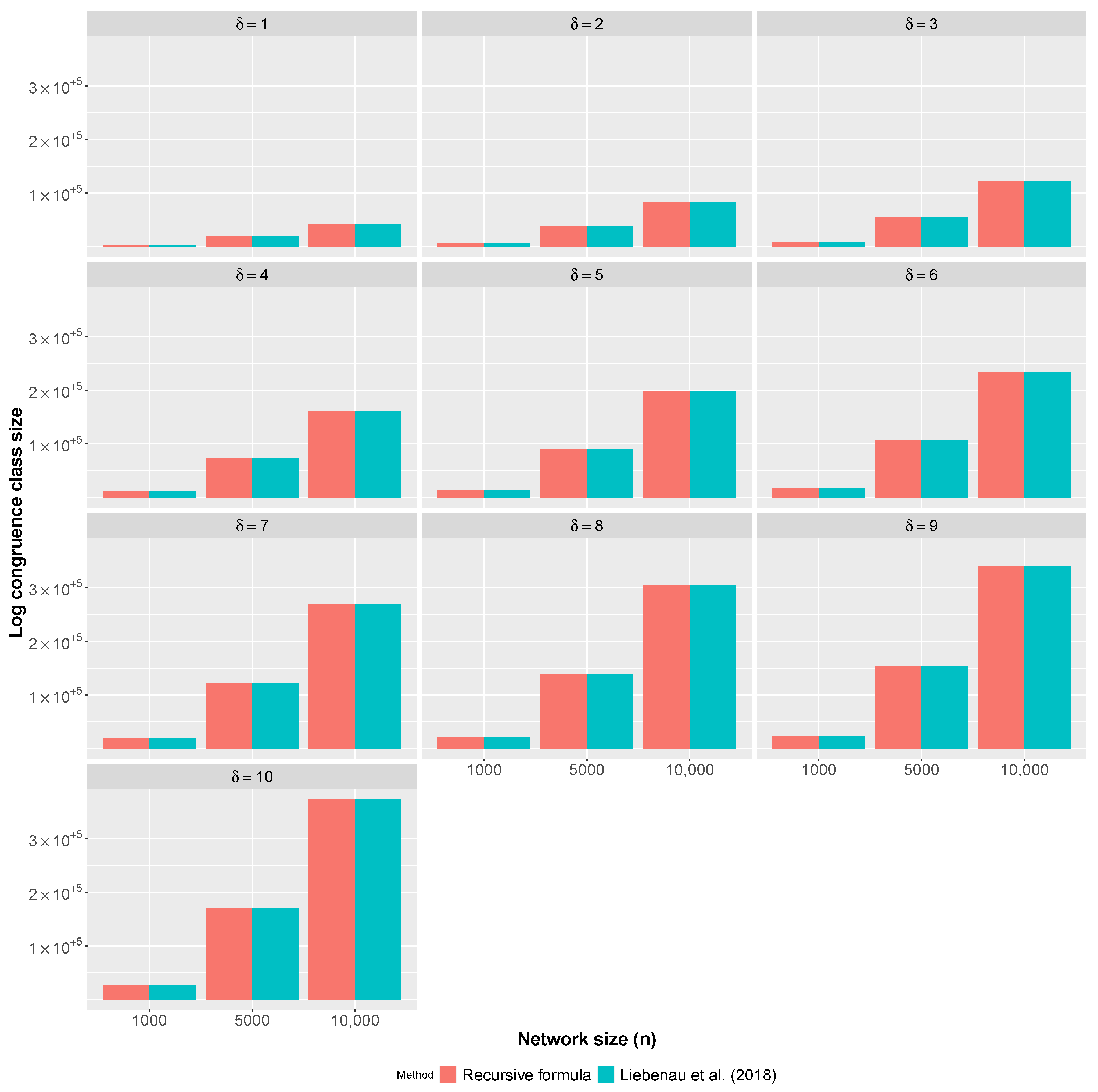
Section 4.2.1 provides a numerical example for calculating $|c_{{\varphi }_{2a}}\left(d_{}^{}\right)|$, while Section 4.2.2 provides a comparison between the presented recursive formula and a formula by Liebenau et al. [9].

3.4. Graph Enumeration Problem: Calculate the Number of Labeled Graphs of Size n with Classification Mixing Matrix ${MM}_{}^{}$

To calculate the number of labeled graphs with mixing matrix ${MM}_{}^{}$, we assume that the classification of all vertices, $M_{}^{}$, is known and ${MM}_{}^{}$ is graphical. We specify $x_0,\dots ,x_k={MM}_{}^{}$ as the following for $l\le m$ ($x_i$ is symmetric):

$$x_{i_{l,m}}^{}=\left\{\begin{array}{c}0 \mathrm{if} i\le {\displaystyle \sum _{a=1}^{l-1}}{\displaystyle \sum _{b=a}^q}{x}_{k_{a,b}}^{}+{\displaystyle \sum _{b=l}^{m-1}}{x}_{k_{l,b}}^{}\hfill \\ x_{k_{l,m}}^{} \mathrm{else} \mathrm{if} i\ge {\displaystyle \sum _{a=1}^{l-1}}{\displaystyle \sum _{b=a}^q}{x}_{k_{a,b}}^{}+{\displaystyle \sum _{b=l}^m}{x}_{k_{l,b}}^{}\hfill \\ i-{\displaystyle \sum _{a=1}^{l-1}}{\displaystyle \sum _{b=a}^q}{x}_{k_{a,b}}^{}+{\displaystyle \sum _{b=l}^{m-1}}{x}_{k_{l,b}}^{}\mathrm{else},\hfill \end{array}\right.$$

(9)

where q is the number of distinct classifications. Theorem 3 proves that there are graphs consistent with $\{x_0,\dots ,x_k\}$ that satisfy $s1-s3$.

Theorem 3.

For a sequence of mixing matrices $\{x_0,\dots ,x_k\}$ defined by Equation (9), there exists a collection of graphs $G_0,\dots ,G_k$ where each consecutive pair satisfies $s1-s3$ for ${\varphi }_3$.

Proof. 

To show this, let $E=\{e_1,\dots ,e_k\}$ be a set of distinct edges where the first $x_{k_{1,1}}^{}$ are between vertices with classification 1, the next $x_{k_{1,2}}^{}$ are between vertices with classification 1 and 2, and so on. Let $G_i$ denote the graph formed with the first i edges from E, i.e., $G_i$ contains edges $\{e_1,\dots ,e_i\}$. Based on the definition of $G_i$, ${\varphi }_3\left(G_i\right)=x_i$, ${\varphi }_3\left(G_{i-1}\right)=x_{i-1}$, and $G_i$ and $G_{i-1}$ differ by a single edge.    □

Let $(v_l,v_j)$ be the single edge that differs between $G_i$ and $G_{i-1}$. Given Theorem 3, $r_{{\varphi }_3}(x_i,x_{i-1})$ is the following:

If $m_l\ne m_j$

$$r_{{\varphi }_3}(x_i,x_{i-1})=\frac{M_{m_l}^{}\times M_{m_j}^{}-x_{i-1_{l,j}}^{}}{x_{i_{l,j}}^{}},$$

(10)

else,

$$r_{{\varphi }_3}(x_i,x_{i-1})=\frac{\left(\genfrac{}{}{0pt}{}{M_{m_l}^{}}{2}\right)-x_{i-1_{l,j}}^{}}{x_{i_{l,j}}^{}},$$

(11)

Using Equations (10) and (11) along with the specification of $x_0,\dots ,x_k={MM}_{}^{}$ as defined above and $|c_{{\varphi }_3}\left(x_0\right)|=1$, it is possible to calculate $|c_{{\varphi }_3}\left({MM}_{}^{}\right)|$.

3.5. Graph Enumeration Problem: Calculate the Number of Graphs of Size n with Degree Mixing Matrix ${DMM}_{}^{}$

To calculate the number of labeled graphs with degree mixing ${DMM}_{}^{}$, we follow a similar approach as that for degree distribution. Specifically, we use a constructive proof for assessing whether a degree mixing matrix is graphical to specify a set of edges, E, that can be used to construct a graph with degree mixing ${DMM}_{}^{}$[13]; Algorithm 2 provides a procedure to construct E.

Algorithm 2: Degree Mixing

Theorem 4.

Let E denote the collection of edges output from Algorithm 2 with a graphical degree mixing matrix ${DMM}_{}^{}$ as input. Let $G_i$ denote the graph formed with the first i edges from E, i.e., contains edges $\{e_1,\dots ,e_i\}$. Let $x_i={\varphi }_4\left(G_i\right)$. Each consecutive pair in the collection of graphs $G_0,\dots ,G_x$ satisfies $s1-s3$ for ${\varphi }_4$.

Proof. 

The edges in E are distinct. Therefore, by design, the conditions are satisfied. □

Based on the definition of $x_0$ in Theorem 4, $|c_{{\varphi }_4}\left(x_0\right)|=1$. Let $(v_l,v_j)$ be the single edge that differs between $G_i$ and $G_{i-1}$. Based on results from Goyal et al. [13]:

$$r_{{\varphi }_4}(x_i,x_{i-1})=\frac{[{\gamma }_1\left(G_{i-1}\right)-{\alpha }_2\left(G_{i-1}\right)]\times {\beta }_{(l,j)}^0\left(G_{i-1}\right)}{{DMM}_{d_l^{}\left(G_i\right),d_j^{}\left(G_i\right)}^{}\left(G_i\right)\times {\beta }_{(l,j)}^1\left(G_i\right)},$$

(12)

where

$${\alpha }_2\left(G\right)={DMM}_{d_l^{}\left(G\right),d_j^{}\left(G\right)}^{}\left(G\right);$$

(13)

$${\gamma }_1\left(G\right)=\left\{\begin{array}{c}{D}_{d_i^{}\left(G\right)}^{}\left(G\right)D_{d_j^{}\left(G\right)}^{}\left(G\right) \mathrm{if} d_i^{}\left(G\right)\ne d_j^{}\left(G\right)\hfill \\ \left(\genfrac{}{}{0pt}{}{D_{d_i^{}\left(G\right)}^{}\left(G\right)}{2}\right)\mathrm{else};\end{array}\right.$$

(14)

and based on concepts from Newman [16], if $d_i^{}\left(z\right)\ne d_j^{}\left(z\right)$,

$${\beta }_{(l,j)}^s\left(G\right)\approx \frac{{\mathsf{\Pi }}_z\left(\genfrac{}{}{0pt}{}{{DMM}_{d_l^{}\left(G\right),z}^{{}^{\prime }}\left(G\right)-I_{\{d_j^{}\left(G\right)=z\}}·s}{n_l^z-I_{\{d_j^{}\left(G\right)=z\}}·s}\right)}{\left(\genfrac{}{}{0pt}{}{{\sum }_z{DMM}_{d_l^{}\left(G\right),z}^{{}^{\prime }}\left(G\right)-I_{\{d_j^{}\left(G\right)=z\}}·s}{d_l^{}\left(G\right)-s}\right)}\times \frac{{\mathsf{\Pi }}_z\left(\genfrac{}{}{0pt}{}{{DMM}_{z,d_j^{}\left(G\right)}^{{}^{\prime }}\left(G\right)-I_{\{d_l^{}\left(G\right)=z\}}·s}{n_j^z-I_{\{d_l^{}\left(G\right)=z\}}·s}\right)}{\left(\genfrac{}{}{0pt}{}{{\sum }_z{DMM}_{z,d_j^{}\left(G\right)}^{{}^{\prime }}\left(G\right)-I_{\{d_l^{}\left(G\right)=z\}}·s}{d_j^{}\left(G\right)-s}\right)}$$

(15)

else,

$${\beta }_{(l,j)}^s\left(G\right)\approx \frac{{\mathsf{\Pi }}_z\left(\genfrac{}{}{0pt}{}{{DMM}_{d_l^{}\left(G\right),z}^{{}^{\prime }}\left(G\right)-I_{\{d_j^{}\left(G\right)=z\}}·s}{n_l^z+n_j^z-2I_{\{d_j^{}\left(G\right)=z\}}·s}\right)}{\left(\genfrac{}{}{0pt}{}{{\sum }_z{DMM}_{d_l^{}\left(G\right),z}^{{}^{\prime }}\left(G\right)-I_{\{d_j^{}\left(G\right)=z\}}·s}{d_l^{}\left(G\right)+d_j^{}\left(G\right)-2s}\right)}.$$

(16)

where ${DMM}_{a,b}^{{}^{\prime }}\left(G\right)={DMM}_{a,b}^{}\left(G\right)$ if $a\ne b$ and ${DMM}_{a,b}^{{}^{\prime }}\left(G\right)=2\ast {DMM}_{a,b}^{}\left(G\right)$ if $a=b$ and $n_l^z$ and $n_j^z$ denote the number of vertices that are neighbors of i and j and equal to z.

Using Equation (12) along with the specification of $x_0,\dots ,x_k={DMM}_{}^{}$ as defined above and $|c_{{\varphi }_4}\left(x_0\right)|=1$, it is possible to calculate $|c_{{\varphi }_4}\left({DMM}_{}^{}\right)|$.

3.6. Additional Graph Properties and Bipartite Graphs

The recursive formula and associated framework we propose can be used to calculate the number of labeled graphs for many additional graph properties. In particular, Goyal et al. [13] provide equations for $r_{\varphi }(x_k,x_{k-1})$ for number of triangles (controlling for degree mixing) as well as jointly specifying classification mixing matrix and degree distribution. In addition, Goyal et al. [17] enables extending the calculation of $r_{\varphi }(x_k,x_{k-1})$ to the setting of bipartite graphs.

4. Results

In this section, we present numerical examples—including validation results for estimating the number of labeled graphs—for two graph properties: number of edges (Section 4.1) and degree sequence (Section 4.2). To the author’s knowledge, our paper is the first to provide formulas for estimating the number of labeled graphs consistent with values for several graph properties (e.g., degree mixing matrix) described in Section 3; hence, for these properties, we are not able to compare our approach to any existing approach. In the application section (Section 5), we present results for the number of labeled graphs associated with particular degree distributions and degree mixing matrices using our presented approach.

4.1. Number of Edges

Although there is a closed-form expression for calculating the number of labeled graphs of size n with m number of edges, we use Equation (1) for calculation of this graph property to illustrate our recursive approach for graph enumeration.

4.1.1. Example

To illustrate the use of the recursive formula, we provide a numerical example where we estimate the number of graphs of size $n=1000$ with exactly $m=10$ edges; that is, we calculate $|c_{{\varphi }_1}(m=10)|$. As discussed in Section 3.1, we set $x_0=0,x_1=1,\dots ,x_k=10$. Therefore, based on Equation (1):

$$|c_{{\varphi }_1}(x_k=10)|=r_{{\varphi }_1}(x_k=10,x_{k-1}=9)·\left|c_{{\varphi }_1}(x_{k-1}=9)\right|.$$

(17)

Based on Equation (3),

$$r_{{\varphi }_1}(x_k=10,x_{k-1}=9)=\frac{\left(\genfrac{}{}{0pt}{}{1000}{2}\right)-9}{10}=49949.1.$$

(18)

Therefore,

$$|c_{{\varphi }_1}(x_k=10)|=49949.1·|c_{{\varphi }_1}(x_{k-1}=9)|.$$

(19)

The next step in the procedure is the calculation of $|c_{{\varphi }_1}(x_{k-1}=9)|$ using the following:

$$|c_{{\varphi }_1}(x_{k-1}=9)|=r_{{\varphi }_1}(x_{k-1}=9,x_{k-2}=8)·\left|c_{{\varphi }_1}(x_{k-2}=8)\right|.$$

(20)

The procedure ends at $x_0=0$. Therefore,

$$log\left(\right|c_{{\varphi }_1}(x_k=10)\left|\right)=\sum _{i=1}^{i=10}log\left(r_{{\varphi }_1}(x_i,x_{i-1})\right)+log\left(\right|c_{{\varphi }_1}(x_0=0)\left|\right).$$

(21)

Table 1. Comparison of methods to calculate number of edges.

x	$\mathit{l}\mathit{o}\mathit{g}\left(\mathit{r}\right(\mathit{x},\mathit{x}-1\left)\right)$	$\mathit{l}\mathit{o}\mathit{g}\left(\right|{\mathit{c}}_{{\mathit{\varphi }}_1}\left(\mathit{x}\right)\left|\right)$	$\mathit{l}\mathit{o}\mathit{g}\left(\right|{\mathit{c}}_{{\mathit{\varphi }}_1}\left(\mathit{x}\right)\left|\right)$
		[Equation (1)]	[Equation (22)]
0	−	0	0
1	$13.12$	$13.12$	$13.12$
2	$12.42$	$25.55$	$25.55$
3	$12.02$	$37.57$	$37.57$
4	$11.74$	$49.31$	$49.31$
5	$11.51$	$60.82$	$60.82$
6	$11.33$	$72.15$	$72.15$
7	$11.18$	$83.32$	$83.32$
8	$11.04$	$94.37$	$94.37$
9	$10.92$	$105.29$	$105.29$
10	$10.82$	$116.11$	$116.11$

provides the log values for $r(x_i,x_{i-1})$ for $i=1$ to 10. Based on these values and noting that $|c_{{\varphi }_1}(x_0=0)|=1$, we calculate $log\left(\right|c_{{\varphi }_1}(x_k=10)\left|\right)=116.11$.

4.1.2. Comparison

To illustrate the validity of the recursive formula in this setting, we compare the estimates of the number of graphs of size n with m edges, $|c_{{\varphi }_1}(m=x)|$, based on the proposed recursive formula to those based on the following existing formula [1]:

$$|c_{{\varphi }_1}\left(x\right)|=\left(\genfrac{}{}{0pt}{}{\left(\genfrac{}{}{0pt}{}{n}{2}\right)}{x}\right).$$

(22)

Our comparison considers values of x ranging from $\{1,\dots ,10\}$ for graphs of size $n=1000$.

For each value of $x\in \{1,\dots ,10\}$, Table 1 provides the log values for $r(x,x-1)$ and $|c_{{\varphi }_1}\left(x\right)|$ based on Equations (1) and (22). The estimates obtained from the proposed recursive formula and the known formula are identical—an expected finding given that a closed-form equation for $r_{{\varphi }_1}(x,x-1)$ exists.

Regarding complexity, computing the recursive formula for $|c_{{\varphi }_1}\left(x\right)|$ requires computing $\left(\genfrac{}{}{0pt}{}{n}{2}\right)$ as well as x number of subtractions and divisions. Therefore, the complexity of the recursive formula is $O\left(x\right)$ where subtractions and divisions are $O\left(1\right)$.

4.2. Degree Sequence

This section illustrates the use of Equation (1) to estimate the number of graphs with a fixed degree sequence.

4.2.1. Example

To illustrate the use of the recursive formula, we provide a numerical example wherein we estimate the number of graphs with $n=1000$ and fixed degree sequence. In particular, we estimate the number of 2-regular graphs of size $n=1000$; a $\delta$-regular graph is one in which each vertex has exactly degree $\delta$. Therefore, the degree sequence for a $\delta$-regular graph is $d_{}^{}=\{\delta ,\dots ,\delta \}$.

As the number of distinct degree sequences for a degree distribution associated with a $\delta$-regular graph is one, Equation (8) simplifies to:

$$|c_{{\varphi }_{2a}}\left(d\right)|=|c_{{\varphi }_2}\left(D_{}^{}\left(d\right)\right)|.$$

(23)

Using Algorithm 1, we generate a sequence of edges E, where E specifies a 2-regular graph of size n. The edge list E contains 1000 edges. A partial list of the edges in E, denoted as a pair consisting of Vertex 1 and Vertex 2 $\in \{1,\dots ,1000\}$, are shown in

Table 2. A partial list of the edges in E, denoted as a pair consisting of Vertex 1 and Vertex 2.

Vertex 1	Vertex 2
$v_1$	$v_2$
$v_1$	$v_3$
$v_4$	$v_5$
$v_4$	$v_6$
…	…
$v_{14}$	$v_{15}$
$v_{11}$	$v_{12}$
$v_8$	$v_9$
$v_5$	$v_6$
$v_2$	$v_3$

. Using the edge list E, we generate a series of graphs, $G_0,\dots ,G_{1000}$, where $G_i$ is the graph that contains the first i edges in E. Next, we generate a series of degree distributions $\{x_0,\dots ,x_{1000}\}$, where $x_i={\varphi }_2\left(G_i\right)$.

Table 3. A partial list of the degree distribution sequences.

Degree 0	Degree 1	Degree 2	Degree 3
$x_0$	1000	0	0	0
$x_1$	998	2	0	0
$x_2$	997	2	1	0
$x_3$	995	4	1	0
$x_4$	994	4	2	0
…	…	…	…	…
$x_{996}$	0	8	992	0
$x_{997}$	0	6	994	0
$x_{998}$	0	4	996	0
$x_{999}$	0	2	998	0
$x_{1000}$	0	0	1000	0

shows a partial list of the degree distribution sequences, i.e., $x_i$. For each consecutive entry in the degree distribution sequences, we can use Equations (4)–(7) to estimate $r_{\varphi }(x_i,x_{i-1})$. As $x_0$ is only consistent with the empty graph, $|c_{{\varphi }_2}\left(x_0\right)|=1$. We estimate the log number of 2-regular graphs as $5907.899$; as we see in the next section an existing formula by Liebenau et al. [9] estimates this as $5907.352$.

4.2.2. Comparison

As in the previous section, we illustrate the validity of the recursive formula in this setting by comparing the estimates of $|c_{{\varphi }_{2a}}\left(d\right)|$ based on the proposed recursive formula to those that result from an existing formula. In particular, we compare results of the proposed recursive approach to those resulting from the available formula for estimating the number of $\delta$-regular graphs of size $n=1000$.

Liebenau et al. [9] proved the validity of a general asymptotic formula—conjectured in 1990—for the number of graphs with given degree sequence. They also provide a formula that converges to the number of $\delta$-regular graphs as $n\to \infty$. This formula allows comparison of $|c_{{\varphi }_{2a}}\left(d\right)|$, where d is the degree sequence $d_{}^{}=\{\delta ,\dots ,\delta \}$, obtained from this asymptotic formula to those from the proposed recursive formula.

Figure 1 shows log estimates for the number of $\delta$-regular graphs for $\delta$ from 1 to 10 for the two approaches. The red bars depict estimates based on the recursive formula introduced in this paper; the blue bars are estimates based on Liebenau et al. [9]. Each plot in Figure 1 shows log estimates for graphs of size 1000, 5000, and 10,000. The log estimates differ by less than $0.01\%$. To calculate the number of graphs with a given degree sequence based on the recursive formula, we first make use of the Havel–Hakimi algorithm, which has a complexity of $O\left(n^2\right)$ [18]. Next, the ratio presented in Equation (4) must be computed $\left({\sum }_{i=1}^{n}d\right)/2$ times, where each calculation of the ratio is $O\left(1\right)$. Finally, we calculate the number of degree sequences that are associated with a degree distribution, which has complexity $O\left(n\right)$. Therefore, the complexity of the recursive formula for calculating the number of graphs of size n with a degree sequence d is $O\left(n^2\right)+O(\left({\sum }_{i=1}^{n}d\right)/2)$.

5. Application

In this section, we estimate the variation in degree mixing matrices consistent with degree distributions formed by the Barabási–Albert (BA) model [10]. The BA model can be initiated with a small seed graph that grows by the addition of new vertices one at a time. Each new vertex forms a new edge with an existing vertex based on preferential attachment rules. Vertices and edges, once introduced, are never deleted. The BA model fixes the number of (undirected) edges connected to each new vertex. The BA model provides a mechanism to generate graphs with a fat-tailed degree distribution—specifically a power-law degree distribution—wherein the probability, $P\left(k\right)$, that a vertex in the graph has degree k, decays as a power-law $P\left(k\right)\sim k^{-\gamma }$.

To calculate the variation in degree mixing matrices consistent with degree distributions formed by the BA model, we first estimate the number graphs consistent with a degree distribution associated with the BA. Second, we estimate the number of graphs consistent with a degree mixing matrix associated with a degree distribution from the BA model. Third, we estimate the number of distinct degree mixing matrices associated with a degree distribution generated from the BA model, which provides a metric for the variation of graphs generated by the BA model.

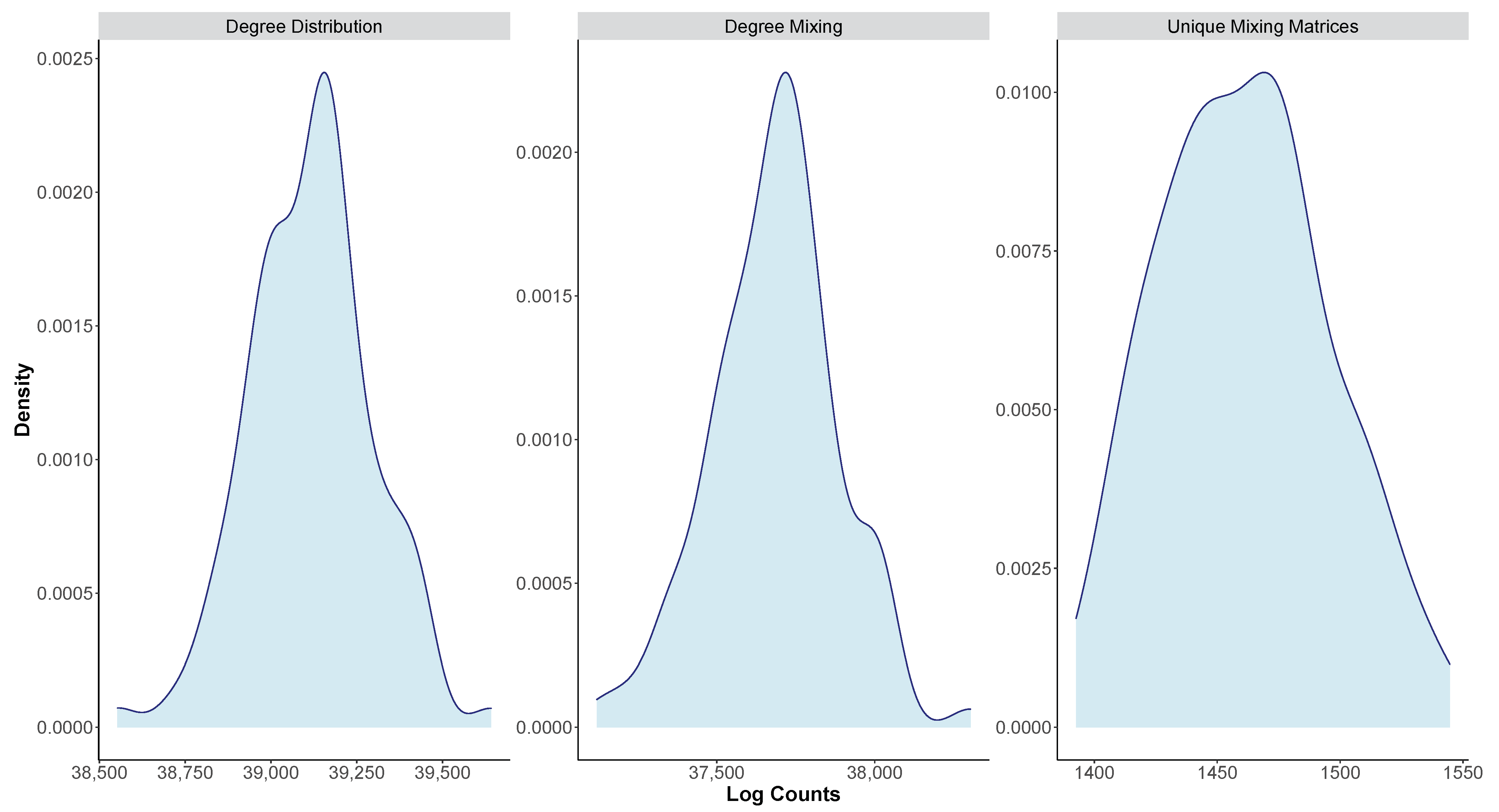
For the first step, we generate 100 graphs using the BA model ($n=5000$), denoted as $\{G_1^{BA},\dots ,G_{100}^{BA}\}$. Figure 2 shows density plots for the log estimates for $|c_{{\varphi }_2}\left({\varphi }_2\left(G_i^{BA}\right)\right)|$ in the first panel. The average number of labeled graphs associated with a degree distribution generated from the BA model was estimated as $1.26e16988$ (exponential of the mean of the first panel in Figure 2). Second, for each graph, we estimate $|c_{{\varphi }_4}\left({\varphi }_4\left(G_i^{BA}\right)\right)|$. Figure 2 (second panel) shows density plots for the log estimates for $|c_{{\varphi }_4}\left({\varphi }_4\left(G_i^{BA}\right)\right)|$. Figure 2 (third panel) shows a density plot for the log estimates for the number of distinct degree mixing matrices associated with a degree distribution generated from the BA model. The exponential of the mean gives an estimate of $4.16e634$ distinct degree mixing matrices associated with a degree distribution generated from the BA model.

6. Discussion

This paper presents a general recursive formula to estimate the number of labeled graphs with specific values for graph properties of interest. We consider those with particular relevance for social network analysis: number of edges (graph density), degree sequence, degree distribution, classification mixing, and degree mixing. The proposed method can easily be extended to additional graph properties, including number of triangles (controlling for degree mixing), as well as to bipartite graphs; the formulas for Equation (2) are currently available. The proposed recursive formula differs from other available approaches for graph enumeration both in its overall approach and in the breadth of graph properties that can be considered; it may be profitable to investigate the theoretical connections between the proposed method and other approaches. Furthermore, graph enumeration has the potential to play an important role in statistical network analysis, because formulating the likelihood of observing a real-world graph with particular properties is necessary for making principled inferences.

One current area of research addresses the question of how to make use of results obtained from a study in one population setting to predict what results of a similar study would have been in a different setting. Causal methodologists refer to such research as the study of transportability. This notion is related to the idea of generalizability of results to populations different from the one under study, but true generalizability requires that two populations be similar in all factors that impact study results in important ways. For example, if characteristics such as age or sex of recipients of interventions impacted their efficacy, then generalizability would require that the two populations be similar in these characteristics. Transportability analyses attempt to adjust for differences in populations in prediction of quantities such as intervention effects in new populations. In the settings we consider, adjustment would be required not only for individual characteristics, but also potentially for graph features that impact intervention effects. For example, if degree assortativity—a summary measure of the degree mixing matrix—impacts the spread of disease or the effectiveness of interventions, then this factor would need to be taken into account when predicting spread or effectiveness in a population different from the one that was studied. The methods we describe would aid in investigation of transportability in such settings by facilitating development of ABM-based simulation studies in which graph properties can be chosen to reflect knowledge about those properties (including their uncertainty) in the setting of interest. Of course, in many settings detailed information about potentially important properties may be unavailable. This issue can be addressed using the methods described above to assess the extent to which the unknown properties might impact intervention effectiveness (or other quantities of interest) in the new population [19]. Ideally it would be safe to exclude these properties from the graph model; but if not, an investigator could use the proposed methods to consider plausible ranges of these properties. Doing so would appropriately increase the uncertainty of the prediction of intervention effectiveness in the new population.