A Model Architecture for Public Transport Networks Using a Combination of a Recurrent Neural Network Encoder Library and a Attention Mechanism

Abstract

This study presents a working concept of a model architecture allowing to leverage the state of an entire transport network to make estimated arrival time (ETA) and next-step location predictions. To this end, a combination of an attention mechanism with a dynamically changing recurrent neural network (RNN)-based encoder library is used. To achieve this, an attention mechanism was employed that incorporates the states of other vehicles in the network by encoding their positions using gated recurrent units (GRUs) of the individual bus line to encode their current state. By muting specific parts of the imputed information, their impact on prediction accuracy can be estimated on a subset of the available data. The results of the experimental investigation show that the full model with access to all the network data performed better in some scenarios. However, a model limited to vehicles of the same line ahead of the target was the best performing model, suggesting that the incorporation of additional data can have a negative impact on the prediction accuracy if they do not add any useful information. This could be caused by poor data quality but also by a lack of interaction between the included lines and the target line. The technical aspects of this study are challenging and resulted in a very inefficient training procedure. We highlight several areas where improvements to our presented method are required to make it a viable alternative to current methods. The findings in this study should be considered as a possible and promising avenue for further research into this novel architecture. As such, it is a stepping stone for future research to improve public transport predictions if network operators provide high-quality datasets.

1. Introduction

A crucial part of making cities more sustainable is the transition from private transport methods to public modes of transport. In cities with existing transport networks, this means that operators need to make their services more attractive to potential passengers. For many patrons, convenience is a key area for improvement [1]. Therefore, it is crucial to improve the estimated arrival time (ETA) predictions, which allow passengers to better plan their journeys. Especially in the case of bus networks, passengers rely heavily on Real-Time Passenger Information (RTPI) systems at bus stops, online, and in mobile apps. Such RTPI systems can be unreliable [2], thus making the bus less attractive as a mode of transport. The UK has seen a steady decline in bus patronage since records began in 1985; bus travel has decreased by a total of 0.7 billion journeys [3]. Because local buses in most areas can only be replaced by private vehicles, this suggests that more passengers opt for their private cars, which can be seen in the steady increase in car traffic on British roads [3]. Taking into account the environmental and social impact of congestion, which causes a substantial waste of energy and human time, this is a troubling trend. Data for 2018/19 show that 4.8 billion bus trips were made in the UK, 58% of all public transport trips [3]. In sum, these travels correspond to an estimated 27.4 billion kilometres travelled and saved approximately 96 million tonnes of CO₂ [4]. In a recent study, the social costs of owning a privately owned SUV were estimated to be close to EUR 1 million if the costs associated with pollution, infrastructure maintenance, and climate are taken into account. This study highlights that the ownership of private vehicles is associated with substantial costs to society and should therefore be reduced [5]. This highlights the importance of making bus networks as attractive as possible to attract travellers who are currently using private cars. If this is achieved, not only will it have a positive environmental impact but will also alleviate congestion issues in urban areas. Additionally, the pandemic has had an impact on the usage of public transport, and operators must restore public confidence in the safety of this mode of transport. Alongside these efforts, reliable ETA predictions will make a difference in the perceived passenger convenience of public transport [6].

We previously noted that the latency of data transmission from buses is caused by the delay in the wireless network infrastructure and the fact that the data in our operational area passes through a number of third-party systems [7]. Consequently, the RTPI system may suggest that the vehicle is further away from a bus stop than it is in reality.

The literature contains a wide range of approaches to predict bus ETAs. These range from more conventional methods such as historic averages [8,9], ARIMA [10] or Kalman Filters [11,12,13,14,15,16]. In general, such methods have low predictive power, and the introduction of Neural Networks (NN) drastically improved the performance of ETA predictions [14,15,16]. In the more recent literature, NN-based approaches have taken centre stage with some impressive results [17], however, further improvements compared to NNs were achieved using hierarchical NNs [18]. A particular focus can be found on RNN structures due to the sequential nature of ETA prediction problems. These methods include Long Short Term Memory (LSTM) networks [19], bidirectional LSTMs [20] or even convolutional LSTMs [21]. However, much more complex methods have become more common and tend to use different types of models for different aspects of the prediction task [22,23,24]. As there is no limit to the complexity of an ETA model somewhat more exotic methods, such as the artificial bee colony algorithm are also represented in the recent literature [25].

As a continuation of our previous work, we investigated possible architectural solutions to capture the interconnectedness of public transport networks and its effects on the accuracy of the prediction. All urban transport networks are, as the name suggests, networks consisting of directly or indirectly connected routes. Disruptions in a specific part of the network can have an impact on vehicles in different areas of the system [26]. Therefore, it is expected that any prediction that is made based on either the entire network or a more extensive part of the network could improve ETA and other predictions. Some examples that address a similar approach are studies that include vehicles on the same route in their prediction, allowing any algorithm to have a better view of the state of the network and thus improving prediction accuracies [27,28,29]. To the best of the author’s knowledge, only one study used true network-based information including some short-term historical data from the entire network in their ETA predictions [30]. Examples from freight networks are more common and have demonstrated that a prediction based on multiple network-based models can improve ETA predictions [31,32]. Another example demonstrates a similar approach for the prediction of taxi ETAs [33].

In sequential data, such as language translation, the so-called attention mechanisms can significantly improve predictive performance. The underlying idea is that the attention head will learn the importance of the order of words in a sentence and will focus more on the important parts of the query. In practice, this is achieved by using an encoder-decoder model with either an attention mechanism in between or a flavour of the attention head that doubles as a decoder. Various versions of attention mechanisms have been described in the recent literature [34,35,36].

In this study, we present a working concept of a model architecture allowing to leverage the state of an entire transport network to make ETA and next-step predictions. To this end a combination of an attention mechanism with a dynamically changing recurrent neural network (RNN) based encoder library. This study presents a pilot investigation into the suitability of this novel model architecture but does not claim superiority. The findings in this study should be considered as a possible and promising avenue for further research into this novel architecture.

2. Methods—Data Processing

To avoid confusion, the term “network” will be used for bus networks and road networks, and all neural networks are hereafter referred to as “models”.

2.1. Data Collection

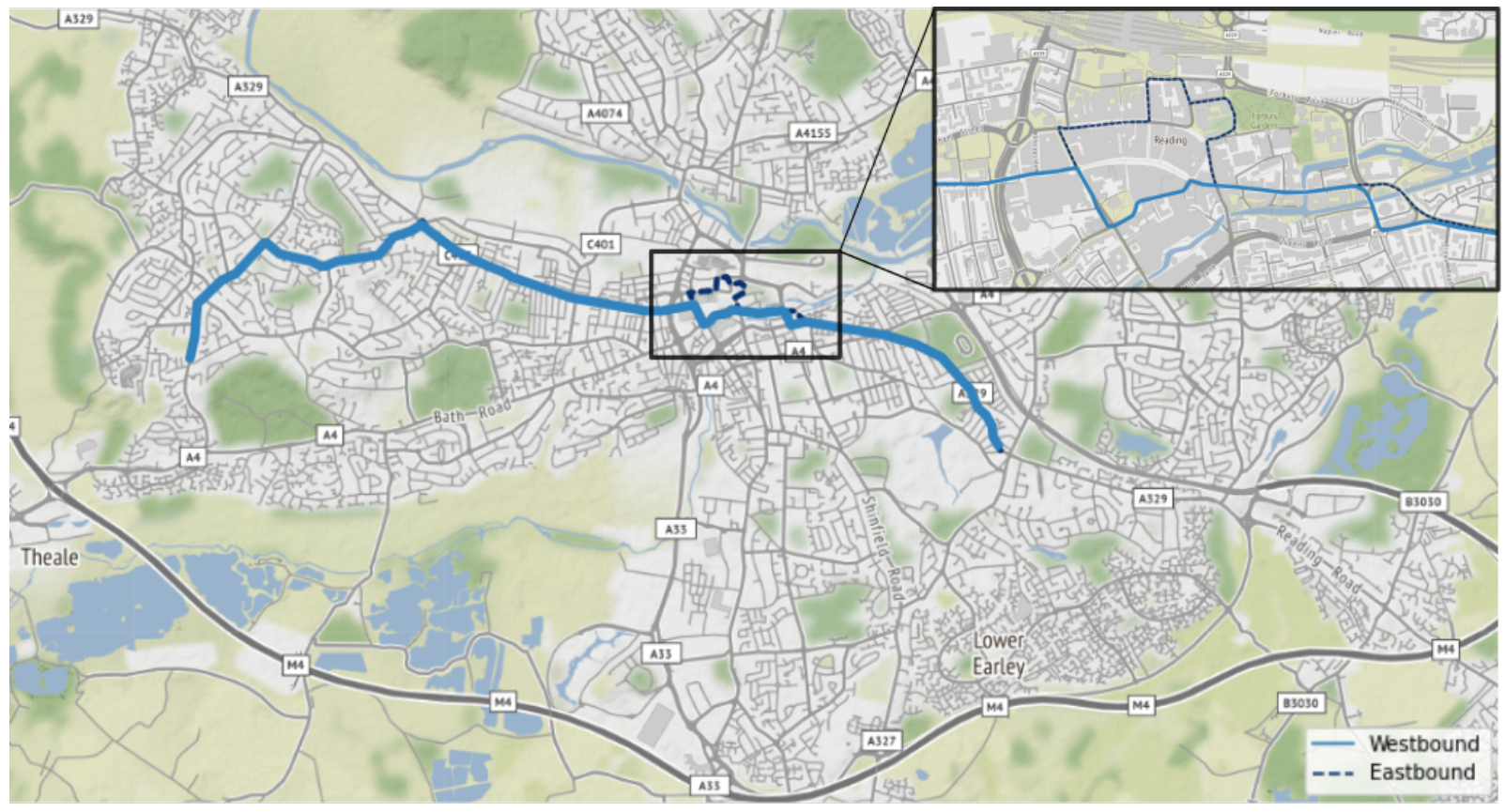
Data were accessed through the infrastructure of our collaborators. For this study, the city Reading (UK) was selected due to the largest amount of available data (Figure 1). As a line of interest, bus line 17 was chosen as it runs with the highest frequency and thus generates the most data. For this line, the predictions were made based on all vehicles which interact with this particular line, see Section 2.2.1. Automatic Vehicle Location (AVL) data were collected for all vehicles within the Reading bus network. Each vehicle sends its position approximately every 40 s, and the company providing the integrated AVL system passes the data on to several third-party entities before it is recorded. Due to the handling of data by several independent companies, only limited amounts of information are transmitted and retained. The available data are as follows.

• Timestamp
• Position (latitude and longitude)
• Line number
• Direction (eastbound or westbound)

Based on this limited information, it is not possible to match the vehicles with the timetables for the current journey. A journey is a specific trip found in the bus line timetables, such as the 9 AM eastbound service. An additional challenge is matching a vehicle to a specific route pattern. These patterns are slightly different routes that a vehicle on the same line might take. On the basis of the available data, a vehicle cannot be matched to such a pattern. Therefore, a route pattern for each city was arbitrarily selected and used to calculate route trajectories, which is an acceptable approach, as in the selected cities the differences between patterns are negligible.

2.2. Data Processing

We have previously described a heuristic method to identify individual journeys, which was applied to the collected data [37]. In summary, it involves the identification of an individual journey based on the change in direction of a vehicle. Then a journey is represented as a trajectory, which is the distance travelled along a route. Finally, the repetitions at the start where the vehicle did not move further than 10 m were removed, and the journey is assumed to start once the vehicle has started moving and ends once the vehicle has reached its destination.

The final dataset included for the westbound direction 113,358 training samples and 24,214 holdout samples and for the eastbound 107,831 and 22,953.

2.2.1. Vehicle Interactions

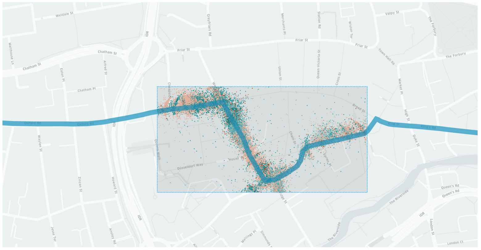
As our hypothesis assumes that additional information can be gained from vehicles which interact with buses on line 17, such interactions should be defined. A road section was selected in the city centre of Reading which poses a bottleneck that most vehicles have to pass. Vehicles passing through the same section as vehicles on line 17 (east or west) were assumed to constitute an interacting line.

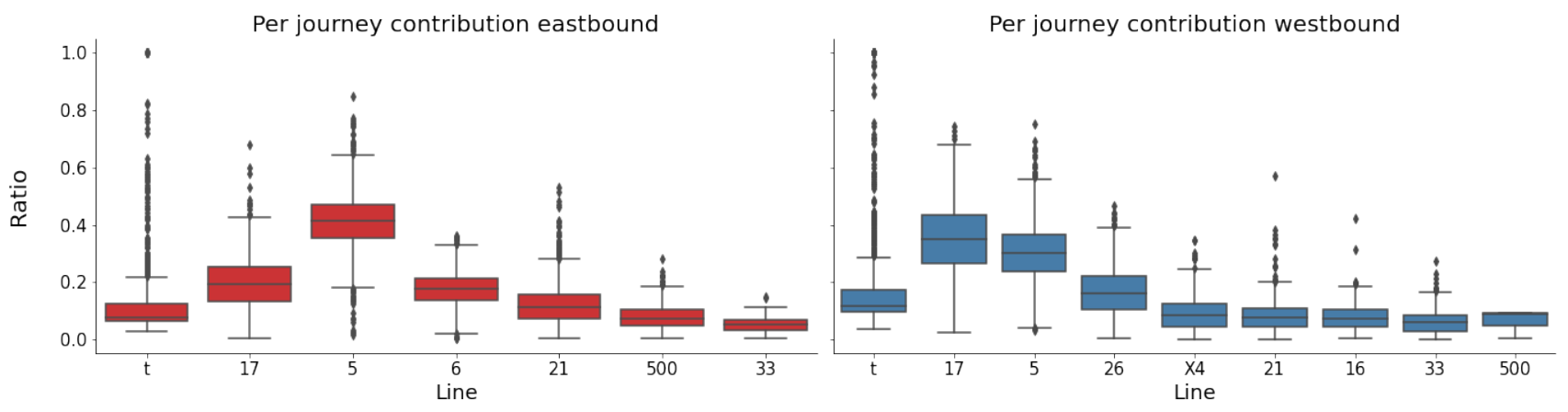
The lines that will be included to test the effect of interactions are identified using an area of interest in the city centre by Reading (Figure 2). A randomly selected subset of 100 k data points are then used to identify lines that travel through this area at any point in time in the same direction as the line of interest. This means that when predicting, for example, line 17 eastbound, not all other lines necessarily are assigned the direction “eastbound” as some might have different starting points, meaning the direction does not match the line of interest.

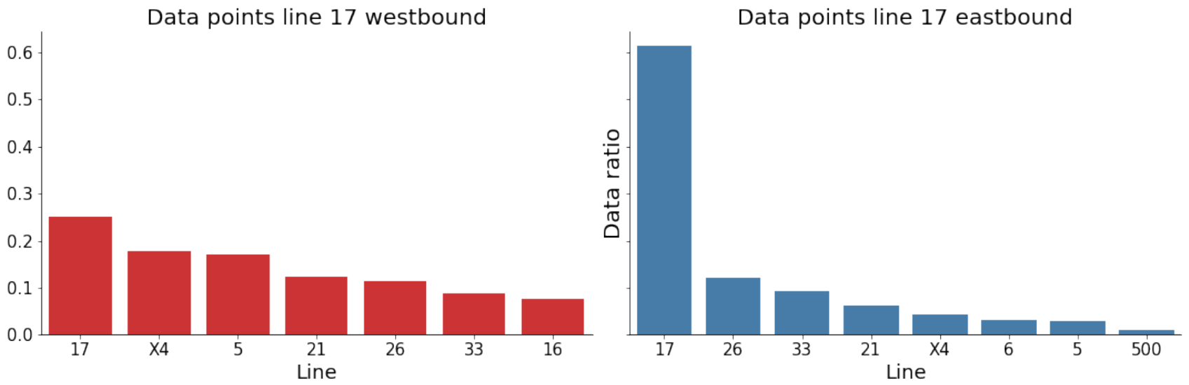
This results in 70 possible lines, of which many only contribute a minuscule fraction. The final selection is made by choosing those lines that contribute more than 3% of the total number of data points in the area of interest Figure 3 and Figure 4.

2.2.2. Input Features

The features included were: coordinates normalised to a bounding box, the bearing reported by the AVL system, the time delta between consecutive recordings, the elapsed time from the start of the journey and time embeddings as described below. The input features were min-max normalised unless stated otherwise.

2.2.3. Time Embeddings

The time information was split into its components to allow algorithms to learn seasonal patterns. To achieve this, the timestamp was translated into minutes of the day, hour of the day, and day of the week. These were embedded in a multidimensional space as detailed in the architecture description.

2.2.4. Target Encoding

Two targets were simultaneously predicted with the reasoning that this might give gradients with richer information and thus could benefit convergence (Section 3.3.6 for details of how the loss was calculated). The first target was an ETA to the final known position. It has to be kept in mind that this could also be a point along the route where a short journey ends and does not necessarily have to be the final stop on the trajectory. This is expressed as minutes from the last data transmission. The second target is the next position along the trajectory, which is equivalent to a fraction along the route and can be decoded to give exact GPS coordinates. As noted previously, reducing the prediction space improves the final prediction. Therefore, the target was expressed as the distance along the trajectory from the last known position, which can be simply added to the previous distance to give a location along the trajectory. This enforces a forward prediction and is more useful, as a vehicle should never change direction in the middle of a journey. The combination of the two targets is an example which is more applicable, as network operators will in most cases be interested in ETA predictions and more accurate vehicle locations.

3. Methods—Model Architecture

Several models and techniques are combined to form a single workflow that accounts for the current state of the entire city network. In the following sections, each individual part is described, followed by a workflow that combines all models into one predictor.

3.1. Line Based Models

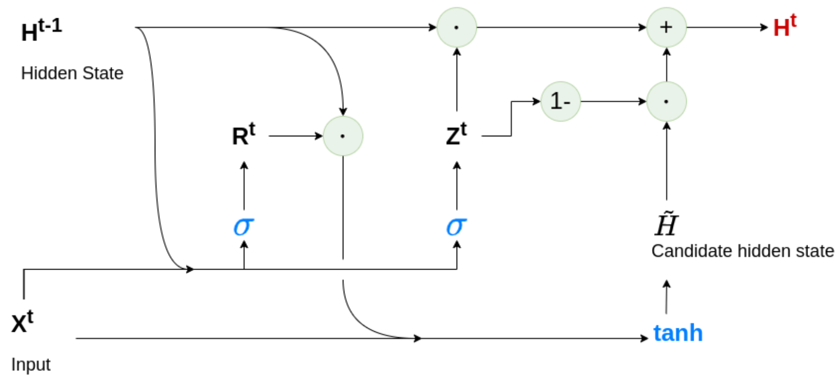
Each included line is assigned a model for both the westbound and eastbound directions. These models are simple Gate Recurrent Units (GRU), Figure 5. Additionally, a separate model was included for the target vehicle, which means that a specific GRU was used for vehicles of line 17, depending on whether they were the target or an interacting vehicle. The time embeddings were learned by the model in a multidimensional space. The dimension is half the possible value of each embedded variable. These 46-dimensional embeddings were fed into a linear layer and reduced to their original dimensions. The output of the linear layer was concatenated with the remaining input features and fed into the GRU. The dimensionality of the output as well as the number of layers was empirically derived based on the training results of a small subset of data (1000 samples). This was necessary due to the very slow training of the model, which will be discussed in Section 3.3.4.

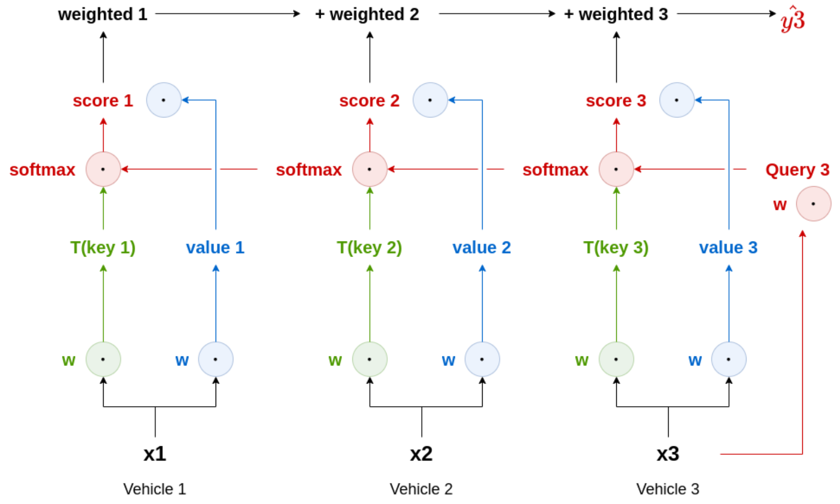
3.2. Attention Mechanism

The outputs of the encoding line-based models are handed over to the decoder, using a user-defined number n of outputs y_t-n from the last n historic network states. These historical network states are used as encoding e to be used by the attention mechanism Figure 6. The first step of the attention mechanism is to derive Queries (Q), Keys (K), and Values (V). To obtain these values, a matrix product is calculated between e and the previously randomly initialised corresponding weights as shown below:

$$Q=e\times W_Q$$

$$K=e\times W_K$$

$$V=e\times W_V$$

where:

e = embedding of user-defined n network states.

$W_Q,W_K,W_V$ = randomly initialised weights for Q, K and V respectively.

The decoder employs a scaled dot product attention as described by [34]. The authors used the following scaling method:

$$Attention(Q,K,V)=softmax\left(\frac{Q{K}^T}{\sqrt{d_k}}\right)V$$

where:

$d_k$ = dimension of queries and keys.

Q, K, V = Queries, Keys and Values respectively.

The authors of [34] hypothesised that the reasons this scaling is necessary are issues caused by vanishing gradients of the softmax layer if the input data of the encoder had high dimensions. We found in our experiments that scaling did worsen the overall performance of the prediction model, and therefore the scaling was abandoned, and a simple dot product attention was modified by upscaling the attention by a constant of 1.5 which was empirically chosen by testing the performance of small subsets of data.

$$Attention(Q,K,V)=softmax\left(Q{K}^{T}c\right)V$$

where:

Q, K, V, c = Queries, Keys, Values and upscaling constant (1.5) respectively.

The output of this attention decoder was fed through a fully connected layer followed by a sigmoid layer to give the final prediction.

3.3. The Training Procedure

The training of this model ensemble is challenging, as it dynamically changes depending on the state of the transport network. At the same time, the weights of a line will be shared between vehicles on the same route and therefore could be accessed several times for each sample. The training procedure is performed in several steps, which are described below in detail. Pytorch [38] was used as the software library of choice.

3.3.1. Initialisation and Optimisation

The GRU initialisation uses a random initialisation with an optional randomness seed for reproducibility for all parameters except for biases. The biases are initialised as zero. All parameters of the attention mechanism are also initialized randomly with the option of providing a seed.

The parameter initialisation for both types of models is performed before the model is defined. This means that in the case of the line GRUs n (n = number of interacting bus lines) sets of parameters are defined. These are stored as a dictionary, which are then loaded into each of the corresponding models. The same procedure is repeated for the attention model.

The handling of these weights poses a technical challenge, as sharing weights between several instances can easily prevent a successful backpropagation. If the parameters are explicitly stored, this causes issues by overwriting the gradients through the inplace operation. This is avoided by the described procedure. As a result, it is possible to leverage Pytorch’s automatic differentiation engine autograd [38]. In practice, this is done by iteratively adding parameters to an optimiser until all parameters of all models are included. This then allows us to backpropagate all models at the same time. Stochastic Gradient Descent [39] was used for this purpose with a momentum of 0.9.

3.3.2. Initial Encoder Pass

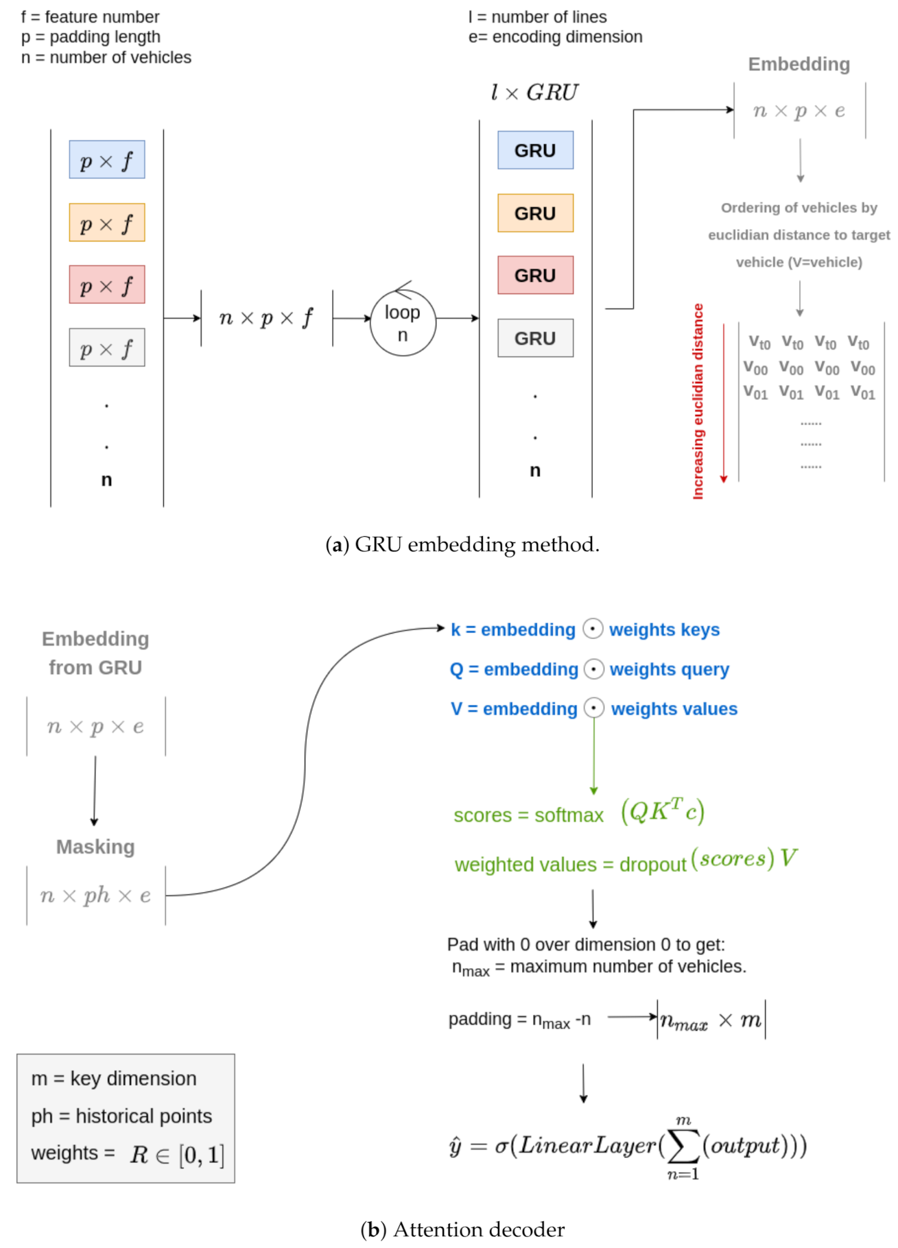
Each sample consists of the last five positions of the interacting bus lines. If fewer positions are available, zero padding is applied. Due to the dynamic nature of the data, where a varying number of vehicles with a varying number of lines make up the input data, an iterative approach for training is required. This means that for each vehicle, the corresponding line model is selected from a dictionary acting as a model library (Figure 7a). This means that if the vehicle is assigned line 3, the line-model number 3 is selected and the vehicle data are passed to this model. The output is temporarily stored for later use in the attention model described in Section 3.3.3. This process is then repeated until all vehicles have been included in the initial training step. The number of vehicles will vary depending on the time of the day and week.

3.3.3. Pass through Attention Decoder

The temporarily stored encoded outputs of the line models are then passed to the attention decoder. The number of historical outputs from positions further in the past can be adjusted to maximise performance. There is no fast rule, and an iterative approach has to be used. The order used was based on the Euclidian distance of the normalised coordinates of all vehicles, where each individual bus is ranked by the distance to the target vehicle. As the interest lies in focusing attention on individual vehicles rather than on the progress of the journey itself, the output is zero-padded to the maximum number of vehicles seen in the dataset (in this example, 24). Although the attention mechanism should be able to account for the order of vehicles, it became apparent through experimental tests that an increase in performance of approximately 30% could be achieved by ordering vehicles. This is necessary to keep the dimension of the weighted values constant to allow them to be fed into the final fully connected layer of the attention mechanism, see Figure 7a,b. This model will return two decimal predictions corresponding to the trajectory of the line of interest (line 17) describing the progress along the route and the time to the final stop. This prediction is stored to be used for the loss calculation at a later point (Section 3.3.4).

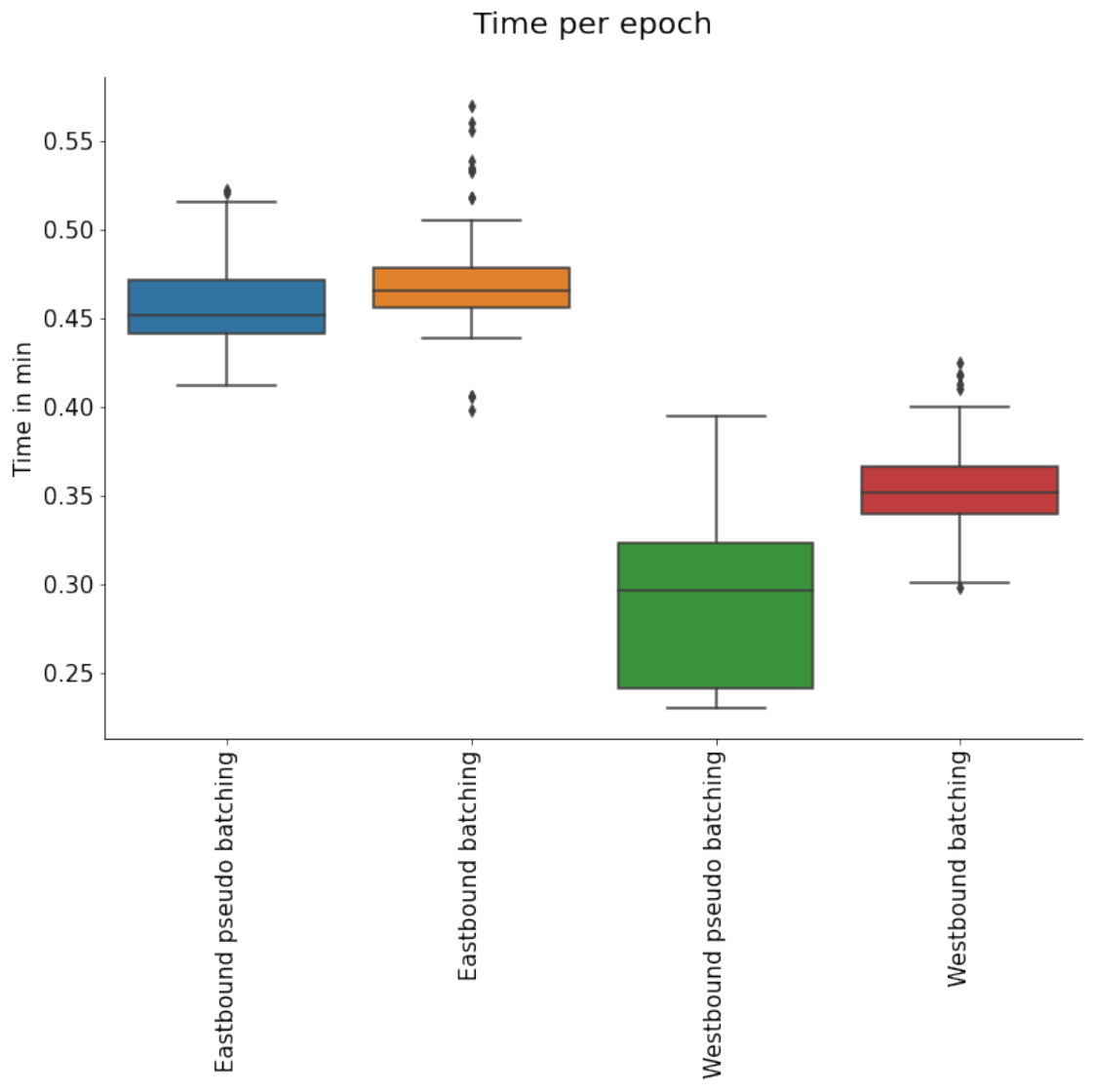
3.3.4. Pseudo-Batching

Due to the complexity of the described training procedure, a true batching of the data is not possible, as the number of underlying line models is dynamic and has to be individually adapted to each sample. Therefore, model training must be done iteratively for each sample. As backpropagation after each sample would cause instability of the model, an alternative was chosen where backpropagation was applied after every 500 samples. This compromise is used to avoid having to wait until the end of an epoch before backpropagation can be run, with the intuition that this should speed up the convergence of the model with fewer epochs needed for training. This method is of course not as effective as true batching, as it cannot leverage the parallel computing capability of a GPU and thus is a very slow process.

3.3.5. Batching

Although true batching is not possible because the composition of the dataset changes for each sample, a batching method was applied to the attention mechanism. To achieve this, the outputs from the line-based GRU models were collected into a batch, which was then handed over to the attention mechanism. This was hypothesised to increase processing speed and improve performance through a regularising effect [40]. To directly compare this batching method with the pseudo-batching method described in Section 3.3.4 equal chunk and batch sizes were used to compare training times.

3.3.6. Loss Calculation and Backpropagation

After a user-defined number of samples, which are considered a pseudo batch, the loss is calculated based on the stored predictions. Due to the initialisation of the optimiser described in Section 3.3.1 the backpropagation can simply be calculated using a single optimiser and will be applied to all models. With the optimised model, a new pseudo-batch can be fed through the model.

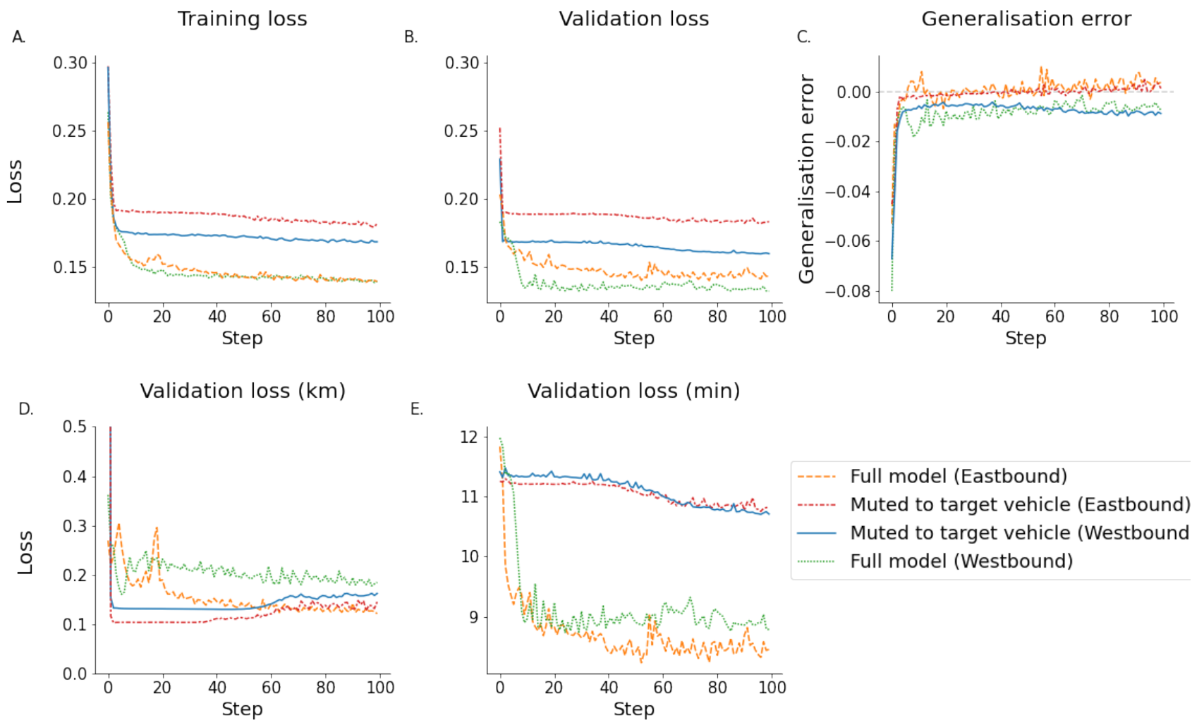
As in this study, two targets are predicted, the next position along the trajectory as well as the time of arrival at the final stop, the Mean Average Error (MAE) is calculated for each metric individually, and both are summed during the training process. This allows to also monitor these individually during training to allow a better evaluation of the training progress.

3.4. Hyper Parameters

Due to the slow training of this model and the large data set, it was not possible to use an automated method such as a gridsearch or a genetic approach to fine-tune the hyperparamaters. Thus, an empirical evaluation was performed using a small subset of the data (3000 randomly selected samples). The convergence speed and final loss for this subset were assessed to make an informed decision on the choice of suitable hyperparameters.

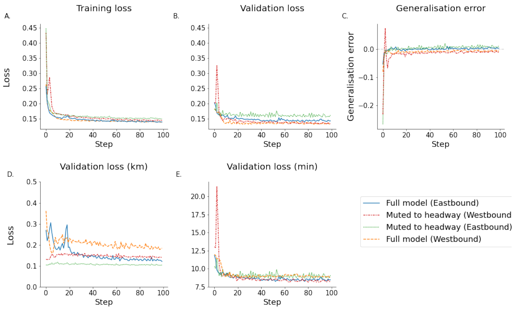
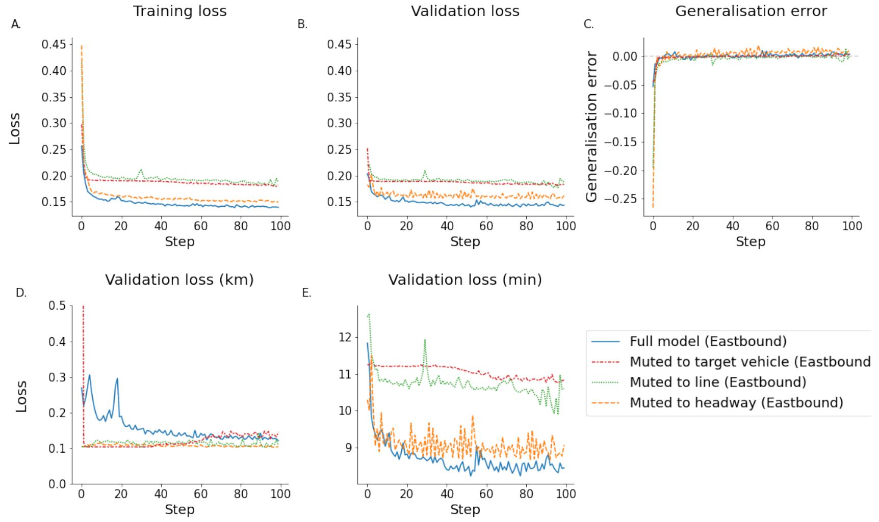
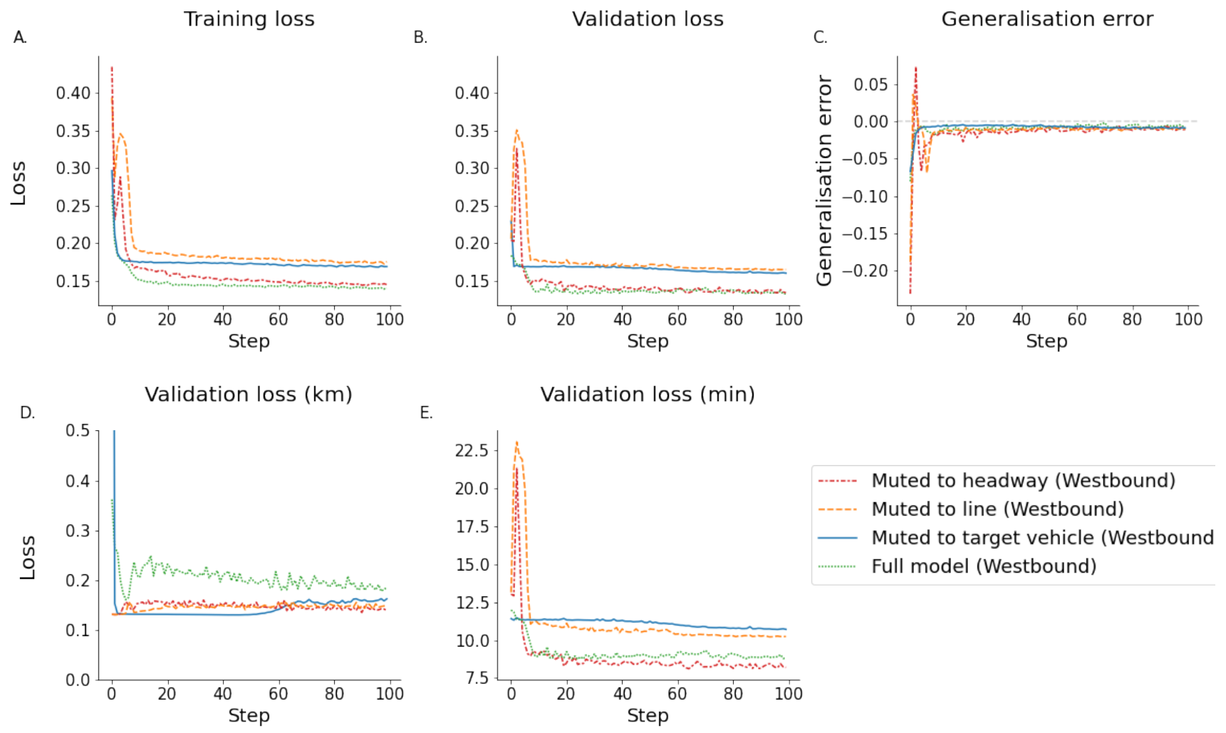
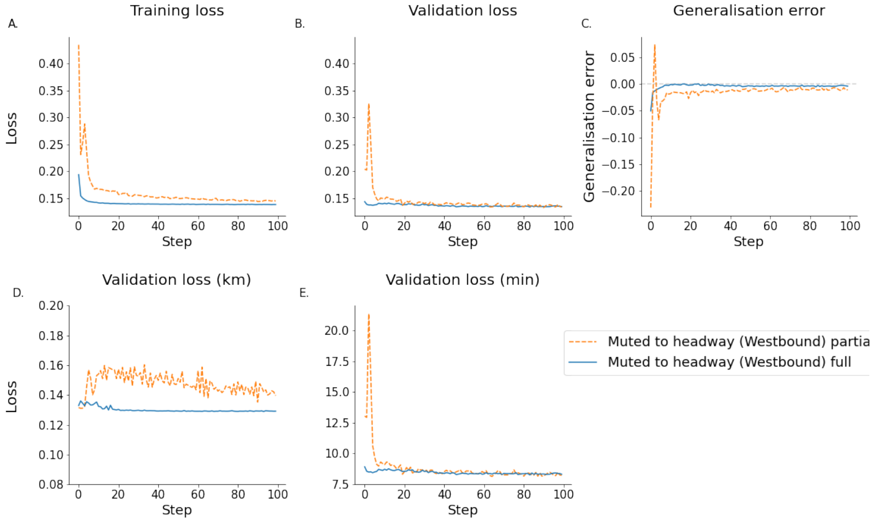
3.5. Performance Evaluation

The calculation of separate losses for both targets allows easy comparison of the loss performance as a whole but also for each target between models. Additionally, the loss distributions were monitored to assess any skewness within the training losses. For any machine learning model, both training and testing losses have to be considered to allow an objective comparison of whether a model generalises well.

3.5.1. Human Interpretable Errors

Furthermore, to make the prediction error more interpretable, the next-step prediction is translated into GPS coordinates based on the shape of the trajectory. This then allows us to calculate the Haversine distance. Note that this will calculate the direct distance and not the distance along the route. Thus, the error could be smaller than the actual distance a vehicle would have to travel along the road.

3.5.2. Generalisation Error

The ultimate goal of most machine learning algorithms is to be generalisable to new unseen data. The ability of an algorithm to generalise can be reduced by overfitting, therefore, the generalisation error was included as a performance metric. The generalisation error is calculated simply by subtracting the training error from the testing error [41]. In a perfectly balanced model, the generalisation error should be towards 0. A negative value indicates a tendency to underfit, while a positive value indicates overfitting.

To highlight the training and testing process of the data subsets, all metrics are shown alongside each other.

4. Results and Discussion

The results shown in the following sections represent training runs on a subset of the data containing 6000 samples. This small subset was chosen due to time constraints due to the inefficient training procedure, which makes training several models on the entire dataset prohibitive due to very long training times. Therefore, the trained models were evaluated on the basis of the training performance of the small dataset. For this reason, both the training loss and the testing loss were used to compare the models and decide on the best performing version for each of the two directions. These models were then trained on the entire dataset and described in Section 4.4.

4.1. Muting of All Vehicles Except Target

A muted model in which only the target vehicle is considered in the prediction was used as a relative comparison to assess whether information from additional vehicles in the network will improve the prediction accuracy of the model. To test this, vehicles were muted during attention application. After the calculation of the weighted values, all values that were not from the target vehicle were multiplied by 0. This removes information about the network state and, as a hypothesis, should perform with lower accuracy compared to the model, which can leverage network information. The results for the eastbound direction showed that on a small subset of the dataset, the addition of network-based information improved the performance of the model, and a model without network information is inferior to the one with the information from the entire bus network (Figure 8) thus confirming the hypothesis. The results are not as clear cut for the westbound direction, where the network-based model outperforms the muted version in ETA prediction, but there is no clear competitive advantage in the trajectory prediction. This can be explained by the fact that the generalisation error remains negative in the training process, suggesting that the model is currently underfitting. This is intuitive if the data contribution of the bus lines shown in Figure 9 is considered, where the proportion of data contributed by target vehicles is greater than in the eastbound direction, which could indicate that longer training times are needed.

4.1.1. Muting of All Vehicles Except Target Line

As a logical continuation of these findings, it can be assumed that if gradually more information is added, this should incrementally improve the model performance. To test this, all vehicles from other lines were muted to include only those running under the same line name and direction. This includes vehicles which will run on earlier schedules than the target vehicle, but also those that follow the target vehicle on later journeys. The results are shown in Figure 10. This modification was compared to the results of the full network-based model and is shown in Section 4.1.3. For both directions, ETA prediction performance was reduced if the model was limited to a single line. However, both directions showed that the muted-line-based model outperformed the full network model. Interestingly, the muted model reached its best performance very quickly, whereas the full model converged slower. These results will be put into context in Section 4.1.3.

4.1.2. Muting of All Vehicles Except Vehicles Ahead of Target

Finally, the focus was on vehicles on the same line, but specifically, only those that are ahead of the target vehicle at their last known position. It would be expected that this will pose an easier problem to model as, based on intuition, the vehicles in front of the target bus will have a more important role compared to those which are following the target. The results are shown in Figure 11 and are compared to the network-based predictor. For both directions, ETA predictions, were not affected by the muting compared to the full model. The muted trajectory prediction was superior to the full model in both directions. However, the generalisation errors for the eastbound direction are more negative than for the westbound direction, suggesting that the model is underfitting in this scenario, see Figure 11.

4.1.3. Summary of Muting Effects

It is expected that the more information about the network is available, the better the performance of the model. This was only partially true. In the experimental investigation, it was shown that the full model with access to all the network data performed better in some scenarios.

However, when the model is limited to the headway, this outperforms the network-based model in both directions of travel for trajectory predictions. It should be noted that the difference between headway and line-limited models in the westbound direction is negligible. The generalisation errors for all models are similar. This makes intuitive sense, as, for example, a delay in a vehicle ahead of the target would most likely translate into a delay for the target vehicle itself. However, a disruption of a vehicle running on a different line might or might not affect the target vehicle. This could be different for instances where several lines run on the same road for longer periods of time. Additional information from the entire network was expected to allow better predictions, as delays in one part of the system could propagate throughout the network and thus eventually affect the target vehicle. This was not the case but could be explained by data quality issues, as discussed before. If the interacting lines are severely affected by quality issues, this could, instead of improving the available information, introduce confusing noise, thus making the prediction less accurate. Furthermore, it could be possible that a different choice of interacting lines could produce better predictions. In the presented example, the lines mostly interact at the end of the journey of the target line when considering the area where both travel on the same stretch of road (see Figure 4). When using lines that run in parallel for longer times, this might improve the importance of the interacting lines. Finally, the choice of target line 17 was made because it is the line with the most available data in the network, which means that the data from the line itself will always outnumber the data from the other lines Figure 9). This results in the fact that the underlying line models of interacting lines will only be updated very infrequently and thus will take much longer to train. Therefore, it can be imagined that if the network-based model was trained for much longer and with more data, it could eventually outperform the headway-limited model.

When assessing the ETA predictions, the results are different, as in the eastbound direction the full model performed best Figure 12, whereas in the westbound direction the headway limited model performed best Figure 13. This is an interesting finding, as the data contribution is different for the two directions. The eastbound direction contains, in addition to the target itself, line number 5 as the most common line (Figure 9). In the westbound direction, the most common line is line 17 (non-target vehicles). This seems to be reflected in the ETA prediction, where the headway limited model performs best in the scenario where the most common data come from line 17 (westbound), whereas in the case where the most common data come from a different line (line 5) the full model performs better Figure 9).

Why this is not found in the trajectory prediction can be explained by the fact that in a setting where other lines contribute more to the data, this can be leveraged by the ETA prediction because intuitively the progress through the network of other lines might affect the final arrival time. In contrast, trajectory prediction is a short-term prediction for the next 40 s only, where the overall network state might be less important. For this example, vehicles immediately ahead of the target will be the most important to make an accurate prediction. This highlights the importance of designing not only a custom method for each line but also for each prediction target.

4.2. Performance of Batching vs. Pseudo-Batching

In an attempt to speed up the model training mechanism, the pseudo-batching method (Section 3.3.4) was compared with the batching method (Section 3.3.5). It should be noted that this batching method only batches the input to the attention mechanism, and due to the complexity of the model selection for each line, it cannot be expected to achieve the same training speed improvements as batching of a conventional model. Furthermore, this experiment was run on an unrestricted prediction space for trajectory prediction, meaning that the model was able to predict any position along the trajectory in contrast to the other experiments discussed where the prediction was limited to points ahead of the last known position. Interestingly, this batching method did not achieve any improvement in training speed, but increased the average processing time required for each epoch by 24% and 4% for the westbound and eastbound directions, respectively (see Figure 14). Considering that the total number of journeys was the same for both conditions, this is a surprising finding but could be explained by the fact that the westbound data are less complex, meaning fewer data points from other lines are included. The eastbound dataset, on the other hand, has a higher proportion of data from other lines and is thus more complex, which could mean that the performance reduction using the GPU processing is less pronounced. It can be hypothesised that although performance was not improved in this dataset, with increasing complexity, GPU processing might become a more efficient training method. This could be useful in a setting that, for example, includes all vehicles at any time in the network.

Although no training speed improvement was observed using this batching method, a benefit of using batching could be that applying batching to the attention mechanism could have a regularising effect on the model gradients [40]. This is due to the phenomenon that very small batch sizes, for example, a single sample as is the case in the pseudo-batching approach, can make the model unstable due to the high variance of the gradient estimates. It should be kept in mind that the line-based GRU models were not batched, and using a method that could apply batching to these models could further increase the model performance. However, this is not possible with the current model architecture.

4.3. Effect of Journey Direction

A complication seen in many of our datasets shows that buses on the same line can have a significantly different route pattern. One cause may be, for example, one-way systems in city centres, which is the case in Reading (Figure 1) and will cause vehicles to travel on different geographical routes depending on the direction. Furthermore, the same line can operate on partial routes and omit certain stops on specific runs. This means in practice that a vehicle of the same line could sometimes stop or start its journey halfway along the route. This complicates any prediction and cannot be extracted from submitted data, as vehicles cannot be matched with specific timetable entries. All investigated bus lines are affected by these conditions, which would be expected to introduce significant and complex noise into the dataset. This issue also makes the interpretation of model performance difficult, as each direction has different timetable patterns, which could affect the difficulty of the prediction task. Furthermore, the westbound direction runs less frequently and therefore produces fewer data points.

4.4. Performance on Full Data

As the results described above show that the model limited to vehicle headways on the same line performs the best in predicting trajectory positions, this version of the model was chosen and ran on a large dataset containing 56,679 and 12,187 training and testing samples for the westbound direction, respectively. In the eastbound direction, the dataset consisted of 107,831 and 22,953 training and testing samples, respectively. In both directions, a moderate improvement in per-epoch validation performance can be noticed. More importantly, a regularisation effect of the larger dataset and consequently a larger number of batches is evident Figure 15 and Figure 16. This can be seen in the less volatile validation curves. A similar reduction in volatility can be seen in the ETA validation performance, especially in the westbound direction. This can be explained by the smaller size of the dataset and, thus, the smaller number of batches within this dataset. From these results, it can be concluded that larger datasets have a two-fold benefit. It results in a reduction in validation volatility and thus generalisation error and, secondly, a moderate improvement of overall prediction performance. This highlights the need for very large datasets if data quality is poor. As a consequence, this results in very long training times. A possibility to further improve the performance of the proposed model structure is to include synthetic data during the training process. This has the caveat that it is unlikely that any network interaction can be incorporated into synthetic models, as these tend to be unknown factors.

4.5. Findings in Context with Previous Results

Both datasets are of different sizes (westbound 12,478 journeys and eastbound 23,960 journeys). As an approximation, we assume a dataset of 12,500 journeys, while our previous paper used 17,115 journeys with an average error of approx. 120 m [7] and showed that this can be improved by incorporating synthetic data [37]. However, because the interacting lines only represent $\approx 5\%$, of the total data this is equivalent to $\approx 625$ journeys for each of the interacting lines. Therefore, to make the dataset equivalent to our previous one for all interacting vehicles, this means the dataset has to be increased by a factor of 27 ($\mathrm{17,000}/625=27$).

Due to the processing time currently needed, this would become prohibitive because of the processing time. A dataset of $\approx \mathrm{12,500}$ requires ≈ 30 min per epoch. If we assume a linear scaling of processing time (this is not fully true as the eastbound dataset does not scale linearly but the run time increases marginally slower than if it was scaling linearly), this then indicates a required epoch time for 30 min ∗ 27 = 13.5 h.

Superconvergence as used in our previous paper by employing the one-cycle policy speeds up the process by approx. 5 fold. This means that the 50 epochs used previously would be equivalent to approximately 250 epochs without a one-cycle policy [41]. As a result, a total processing time of 140 d can be expected, making such an experiment prohibitive.

It should be noted that these values are based on the number of data points in the area of interest as defined in Figure 2 and therefore represent only a small part of the traffic system. Another way to look at the problem would be to assess the percentages of data points in the final dataset. These show a different picture as each vehicle can be found in several samples for different target vehicles. This means that data points related to a target vehicle can be outnumbered by data points from other lines. This means concretely that more data for interacting lines can be present, thus it can be assumed that if more data from the target line were present, this could further improve the model accuracy.

5. Future Work

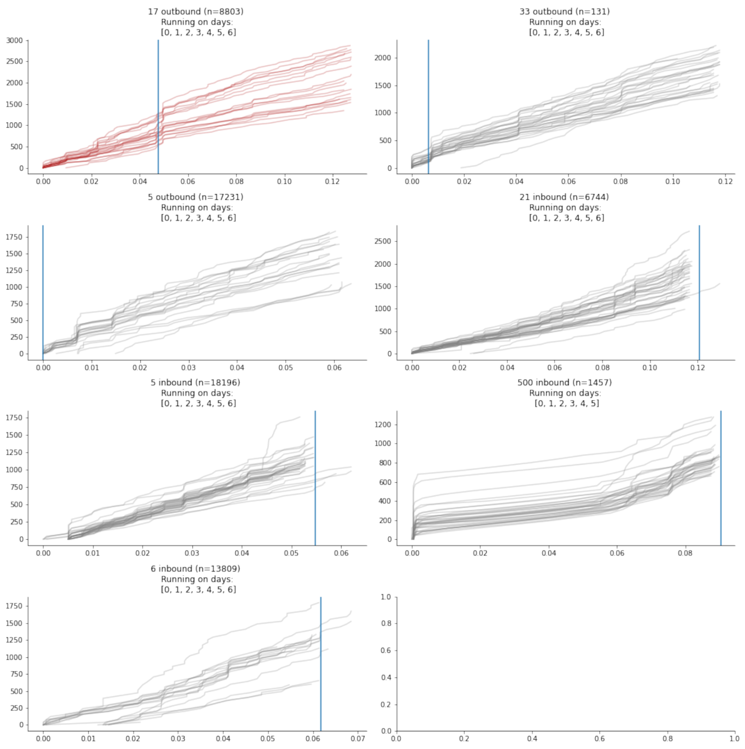
This study highlighted that, in some cases, a network-wide attention-based prediction method can improve ETA, as well as next-step location prediction. It also showed some drawbacks of this method, such as the complexity of implementation due to the fact that many but dynamically changing numbers of models have to be trained in parallel. This made the process computationally very inefficient and, thus, in the current state of research, not a viable alternative to conventional models. The complexity of model training prevented an efficient way of batching training samples. The single most important continuation of this work would be the implementation of a batching method, which not only speeds up training, making the development of a prediction algorithm less computationally costly, but might also improve the generalisation due to a regularising effect. If this is implemented efficiently, this should also allow the use of GPUs to further improve processing times. Another limitation of this study is the definition of what constitutes an interaction between lines. Ideally, all vehicles within the network should be included to prevent suboptimal bias in the choice of lines to be included in the model. Due to the highlighted high computational cost, this is currently not feasible. Once the aforementioned training inefficiencies are addressed, this will become possible and could boost prediction performance. Another issue related to the choice of interacting lines is the fact that most of these interact at the end of the journey of line number 17 as shown in Figure 4. This means that the interaction between the lines is short-lived and might not have a large effect on the prediction accuracy. This could be alleviated by either choosing a different target line other than line 17 or modifying the selection criteria and definition of interacting lines. Furthermore, hyperparameter tuning was conducted empirically due to processing cost and only on a small subset of the data. Ideally, a hyperparameter search should be conducted on the entire dataset if possible, using a gridsearch or potentially a genetic approach. However, due to the extremely long processing time, this is currently prohibitive. Finally, as we have highlighted before, our dataset has serious data quality issues [7]. As these issues are caused by infrastructure problems, these could be easily addressed if all involved companies prioritised their data collection and processing methods and made these publicly available.

6. Conclusions

To summarise, we have demonstrated the potential benefit of a novel model architecture using network-wide data to make predictions in public transport networks. The method developed is based on a library of GRU models for each individual line within a network to embed the temporal information of the individual vehicles. The combination of this embedding method with a transformer model allows the presented method to expand its information range to other vehicles within a bus network. The results are especially promising if vehicles ahead of the target vehicle are included. As this is a pilot study and was designed to test whether the described architecture is a promising area of research, more work is required to compare this architecture to more conventional methods. We have also highlighted several areas where improvements to our presented method are required to make it a viable alternative to current methods. As such, it is a stepping stone for future research to improve public transport predictions if network operators provide high-quality datasets. Furthermore, the developed method could also be used to simulate specific traffic scenarios, such as delays of specific vehicles and the effect on the rest of the bus network. Therefore, the presented method could not only result in better predictions, but could be a valuable simulation tool for network operators.

References

1. Peek, G.J.; van Hagen, M. Creating Synergy In and Around Stations: Three Strategies for Adding Value. Transp. Res. Rec. J. Transp. Res. Board 2002, 1793, 1–6. [Google Scholar] [CrossRef]
2. Salvador, M.M.; Budka, M.; Quay, T. Automatic Transport Network Matching Using Deep Learning. Transp. Res. Procedia 2018, 31, 67–73. [Google Scholar] [CrossRef]
3. Department for Transport. Transport Statistics Great Britain 2019 Moving Britain Ahead; Technical Report; Department for Transport: London, UK, 2019. [Google Scholar]
4. Department for Business Energy & Industrial Strategy. Greenhouse Gas Reporting: Conversion Factors 2019; Department for Business Energy & Industrial Strategy: London, UK, 2019. [Google Scholar]
5. Gössling, S.; Kees, J.; Litman, T. The lifetime cost of driving a car. Ecol. Econ. 2022, 194, 107335. [Google Scholar] [CrossRef]
6. Mishalani, R.G.; Mccord, M.M.; Wirtz, J. Passenger Wait Time Perceptions at Bus Stops: Empirical Results and Impact on Evaluating Real- Time Bus Arrival Information. J. Public Tr. 2006, 9, 89–106. [Google Scholar] [CrossRef]
7. Reich, T.; Budka, M.; Hulbert, D. Impact of Data Quality and Target Representation on Predictions for Urban Bus Networks. In Proceedings of the 2020 IEEE Symposium Series on Computational Intelligence, SSCI 2020, Canberra, Australia, 1–4 December 2020; pp. 2843–2852. [Google Scholar] [CrossRef]
8. Meng, L.; Li, P.; Wang, J.; Zhou, Z. Research on the Prediction Algorithm of the Arrival Time of Campus Bus. In Proceedings of the 2017 International Conference on Information Technology and Intelligent Manufacturing (ITIM 2017), Zhengzhou, China, 5–6 August 2017; pp. 31–33. [Google Scholar]
9. Maiti, S.; Pal, A.; Pal, A.; Chattopadhyay, T.; Mukherjee, A. Historical Data based Real Time Prediction of Vehicle Arrival Time. In Proceedings of the 17th International IEEE Conference on Intelligent Transportation Systems (ITSC), Qingdao, China, 8–11 October 2014; pp. 1837–1842. [Google Scholar] [CrossRef]
10. Napiah, M.; Kamaruddin, I. Arima Models for Bus Travel Time Prediction. J. Inst. Eng. 2009, 71, 49. [Google Scholar]
11. Dailey, D.; Maclean, S.; Cathey, F.; Wall, Z. Transit Vehicle Arrival Prediction: Algorithm and Large-Scale Implementation. Transp. Res. Rec. J. Transp. Res. Board 2001, 1771, 46–51. [Google Scholar] [CrossRef]
12. Cathey, F.W.; Dailey, D.J. A prescription for transit arrival/departure prediction using automatic vehicle location data. Transp. Res. Part C Emerg. Technol. 2003, 11, 241–264. [Google Scholar] [CrossRef]
13. Padmanaban, R.P.S.; Vanajakshi, L.; Subramanian, S.C. Estimation of bus travel time incorporating dwell time for APTS applications. In Proceedings of the IEEE Intelligent Vehicles Symposium Proceedings, Xi’an, China, 3–5 June 2009; pp. 955–959. [Google Scholar] [CrossRef]
14. Shalaby, A.; Farhan, A. Bus Travel Time Prediction Model for Dynamic Operations Control and Passenger Information Systems. In Proceedings of the CD-ROM. Transportation Research Board 82nd Annual Meeting, National Research Council, Washington, DC, USA, 12–16 January 2003. [Google Scholar]
15. Shalaby, A.; Farhan, A. Prediction model of bus arrival and departure times using AVL and APC data. J. Public Transp. 2004, 7, 41–61. [Google Scholar] [CrossRef] [Green Version]
16. Vanajakshi, L.; Subramanian, S.; Sivanandan, R. Travel time prediction under heterogeneous traffic conditions using global positioning system data from buses. IET Intell. Transp. Syst. 2009, 3, 1. [Google Scholar] [CrossRef]
17. Treethidtaphat, W.; Pattara-Atikom, W.; Khaimook, S. Bus arrival time prediction at any distance of bus route using deep neural network model. In Proceedings of the 2017 IEEE 20th International Conference on Intelligent Transportation Systems (ITSC), Yokohama, Japan, 16–19 October 2017; pp. 988–992. [Google Scholar] [CrossRef]
18. Lin, Y.; Yang, X.; Zou, N.; Jia, L. Real-Time Bus Arrival Time Prediction: Case Study for Jinan, China. J. Transp. Eng. 2013, 139, 1133–1140. [Google Scholar] [CrossRef]
19. Zeng, L.; He, G.; Han, Q.; Ye, L.; Li, F.; Chen, L. A LSTM based bus arrival time prediction method. In Proceedings of the 2019 IEEE SmartWorld, Ubiquitous Intelligence and Computing, Advanced and Trusted Computing, Leicester, UK, 19–23 August 2019; pp. 544–549. [Google Scholar] [CrossRef]
20. Nadeeshan, S.; Perera, A.S. Multi-step bidirectional LSTM for low frequent bus travel time prediction. In Proceedings of the MERCon 2021—7th International Multidisciplinary Moratuwa Engineering Research Conference, Virtual Conference, 27–29 July 2021; pp. 462–467. [Google Scholar] [CrossRef]
21. Xie, Z.Y.; He, Y.R.; Chen, C.C.; Li, Q.Q.; Wu, C.C. Multistep Prediction of Bus Arrival Time with the Recurrent Neural Network. Math. Probl. Eng. 2021, 2021, 6636367. [Google Scholar] [CrossRef]
22. Liu, H.; Schneider, M. Similarity measurement of moving object trajectories. In Proceedings of the Third ACM SIGSPATIAL International Workshop on GeoStreaming—IWGS ’12, Redondo Beach, CA, USA, 6 November 2012; pp. 19–22. [Google Scholar] [CrossRef]
23. Nimpanomprasert, T.; Xie, L.; Kliewer, N. Comparing two hybrid neural network models to predict real-world bus travel time. Transp. Res. Procedia 2022, 62, 393–400. [Google Scholar] [CrossRef]
24. Petersen, N.C.; Rodrigues, F.; Pereira, F.C. Multi-output Deep Learning for Bus Arrival Time Predictions. Transp. Res. Procedia 2019, 41, 138–145. [Google Scholar] [CrossRef]
25. Wu, X.; Huang, S.; Zou, J.; Shen, J.; Cai, W.; Zhao, J. Bus Arrival Time Estimation Based on GPS Data by the Artificial Bee Colony Optimization BP Neural Network. In Proceedings of the 2020 5th International Conference on Smart Grid and Electrical Automation, ICSGEA 2020, Zhangjiajie, China, 13–14 June 2020; pp. 264–267. [Google Scholar] [CrossRef]
26. Cats, O.; Jenelius, E. Beyond a complete failure: The impact of partial capacity degradation on public transport network vulnerability. Transp. B 2018, 6, 77–96. [Google Scholar] [CrossRef]
27. Yu, B.; Lam, W.H.K.; Tam, M.L. Bus arrival time prediction at bus stop with multiple routes. Transp. Res. Part C Emerg. Technol. 2011, 19, 1157–1170. [Google Scholar] [CrossRef]
28. Hua, X.; Wang, W.; Wang, Y.; Ren, M. Bus arrival time prediction using mixed multi-route arrival time data at previous stop. Transport 2017, 33, 1–12. [Google Scholar] [CrossRef]
29. Bai, C.; Peng, Z.R.; Lu, Q.C.; Sun, J. Dynamic bus travel time prediction models on road with multiple bus routes. Comput. Intell. Neurosci. 2015, 2015. [Google Scholar] [CrossRef]
30. Čelan, M.; Lep, M. Bus-arrival time prediction using bus network data model and time periods. Future Gener. Comput. Syst. 2020, 110, 364–371. [Google Scholar] [CrossRef]
31. Balster, A.; Hansen, O.; Friedrich, H.; Ludwig, A. An ETA Prediction Model for Intermodal Transport Networks Based on Machine Learning. Bus. Inf. Syst. Eng. 2020, 62, 403–416. [Google Scholar] [CrossRef]
32. Poschmann, P.; Weinke, M.; Balster, A.; Straube, F.; Friedrich, H.; Ludwig, A. Realization of ETA Predictions for Intermodal Logistics Networks Using Artificial Intelligence. Lect. Notes Logist. 2019, 2, 155–176. [Google Scholar] [CrossRef]
33. Paliwal, C.; Biyani, P. To each route its own ETA: A generative modeling framework for ETA prediction. In Proceedings of the 2019 IEEE Intelligent Transportation Systems Conference, ITSC 2019, Auckland, NZ, USA, 27–30 October 2019; pp. 3076–3081. [Google Scholar] [CrossRef]
34. Vaswani, A.; Shazeer, N.; Parmar, N.; Uszkoreit, J.; Jones, L.; Gomez, A.N.; Kaiser, L.; Polosukhin, I. Attention Is All You Need. Vis. Neurosci. 2017, 31, 153–163. [Google Scholar] [CrossRef]
35. Tang, G.; Müller, M.; Rios, A.; Sennrich, R. Why self-attention? A targeted evaluation of neural machine translation architectures. In Proceedings of the 2018 Conference on Empirical Methods in Natural Language Processing, EMNLP 2018, Brussels, Belgium, 31 October–4 November 2018; pp. 4263–4272. [Google Scholar] [CrossRef] [Green Version]
36. Elbayad, M.; Besacier, L.; Verbeek, J. Pervasive Attention: 2D Convolutional Neural Networks for Sequence-to-Sequence Prediction. arXiv 2018, arXiv:1808.03867v2. [Google Scholar]
37. Reich, T.; Budka, M.; Hulbert, D. Bus journey simulation to develop public transport predictive algorithms. Soft Comput. Lett. 2021, 3, 100029. [Google Scholar] [CrossRef]
38. Paszke, A.; Gross, S.; Massa, F.; Lerer, A.; Bradbury, J.; Chanan, G.; Killeen, T.; Lin, Z.; Gimelshein, N.; Antiga, L.; et al. PyTorch: An imperative style, high-performance deep learning library. Adv. Neural Inf. Process. Syst. 2019, 32, 12. [Google Scholar]
39. Kiefer, J.; Wolfowitz, J. Stochastic Estimation of the Maximum of a Regression Function. Ann. Math. Stat. 1952, 23, 462–466. [Google Scholar] [CrossRef]
40. Goodfellow, I.; Bengio, Y.; Courvill, A. Deep Learning (Adaptive Computation and Machine Learning Series); MIT Press: Cambridge, MA, USA, 2016. [Google Scholar]
41. Smith, L.N. A disciplined approach to neural network hyper-parameters: Part 1—Learning rate, batch size, momentum, and weight decay. arXiv 2018, arXiv:1803.09820. [Google Scholar]
Figure 1. Map of Reading showing both the Eastbound as well as Westbound journey patterns. The blow-out area shows the city centre where the line negotiates a one-way system and therefore, runs on two separate routes depending on the direction of travel.
Algorithms 15 00328 g001
Figure 2. Map of the Reading city centre showing the route of the eastbound line 17 in blue with a square indicating the area of interest where the selection of additional lines to be included in the model was made.
Algorithms 15 00328 g002
Figure 3. Ratio of data contribution for both directions an their interacting lines. Only those lines are shown which contribute more than 3% of data points in the area of interests as shown in Figure 2. Left shows the ratio of data points to the target line with origin from each of the included lines for the westbound direction. Right shows the ratio of data points to the target line for the eastbound direction.
Algorithms 15 00328 g003
Figure 4. Interacting line trajectories blue line is the are of interaction from Figure 2, red trajectories are the line of interest in this case line 17 eastbound.
Algorithms 15 00328 g004
Figure 5. The architecture of a single GRU cell where: H t 1 = previous hidden state ; R = Reset gate = σ ( x t ) · W x + H t 1 · W h r + b r ; Z = Update gate = σ ( x t ) · W x z + H t 1 · W h z + b z ; H = Hidden state = t a n h ( x t · W x h ) + ( R · H t 1 ) · W h ; y ^ = Output = H t + W h q + b q .
Algorithms 15 00328 g005
Figure 6. Schema of attention without fully connected layer or sigmoid. This illustrates the attention mechanism itself.
Algorithms 15 00328 g006
Figure 7. (a) GRU embedding method where each vehicle input is iterative fed into the corresponding line model to then generate the embedding matrix with the embedding dimension e. (b) Attention decoder for a single embedding shown in figure a. This shows the generation of keys, values and scores as well as the weighting of the and finally the generation of the final output.
Algorithms 15 00328 g007
Figure 8. These figures show the model mutedto the target vehicle itself thus removing all external information. This is compared to network-based model clearly showing that the performance is reduced if the model does not have access to any external data. (A) shows the training loss. (B) shows the validation loss. (C) shows the generalisation error calculated by subtracting the training error from the testing error. (D) shows the estimated validation error in km. (E) shows the estimated validation loss in minutes. (Note that subfigure (D) has a truncated y axis for illustration purposes).
Algorithms 15 00328 g008
Figure 9. Per journey data composition of 1000 randomly selected journeys.
Algorithms 15 00328 g009
Figure 10. These figures show the model muted to vehicles of the same line regardless of their location in relation to the target vehicle. This is compared to network-based model clearly showing that the performance is reduced if the model does only have access to indiscriminate information of its own line. (A) shows the training loss. (B) shows the validation loss. (C) shows the generalisation error calculated by subtracting the training error from the testing error. (D) shows the estimated validation error in km. (E) shows the estimated validation loss in minutes. (Note that subfigure (D) has a truncated y axis for illustration purposes).
Algorithms 15 00328 g010
Figure 11. The model was muted to the headway meaning only vehicles ahead of the target were included. This shows a clear performance increase in both the training an testing dataset for both directions.(A) shows the training loss. (B) shows the validation loss. (C) shows the generalisation error calculated by subtracting the training error from the testing error. (D) shows the estimated validation error in km. (E) shows the estimated validation loss in minutes. (Note that subfigure (D) has a truncated y axis for illustration purposes).
Algorithms 15 00328 g011
Figure 12. Training and validation of the eastbound direction for all muted models in comparison to the model with access to the entire network data. In the example of this direction the best validation loss was achieved by the model incorporating the entire network data. (A) shows the training loss. (B) shows the validation loss. (C) shows the generalisation error calculated by subtracting the training error from the testing error. (D) shows the estimated validation error in km. (E) shows the estimated validation loss in minutes. (Note that subfigure (D) has a truncated y axis for illustration purposes).
Algorithms 15 00328 g012
Figure 13. Training and validation of the westbound direction for all muted models in comparison to the model with access to the entire network data.In the example of this direction the best validation loss was achieved by the model incorporating the entire network data. (A) shows the training loss. (B) shows the validation loss. (C) shows the generalisation error calculated by subtracting the training error from the testing error. (D) shows the estimated validation error in km. (E) shows the estimated validation loss in minutes. (Note that subfigure (D) has a truncated y axis for illustration purposes).
Algorithms 15 00328 g013
Figure 14. Figure shows boxplots of the time per epoch for both directions.
Algorithms 15 00328 g014
Figure 15. Comparison of the westbound headway muted model trained on a partial as well as a full dataset. (A) shows the training loss. (B) shows the validation loss. (C) shows the generalisation error calculated by subtracting the training error from the testing error. (D) shows the estimated validation error in km. (E) shows the estimated validation loss in minutes. (Note that subfigure (D) has a truncated y axis for illustration purposes).
Algorithms 15 00328 g015
Figure 16. Comparison of the eastbound headway muted model trained on a partial as well as a full dataset.(A) shows the training loss. (B) shows the validation loss. (C) shows the generalisation error calculated by subtracting the training error from the testing error. (D) shows the estimated validation error in km. (E) shows the estimated validation loss in minutes. (Note that subfigure (D) has a truncated y axis for illustration purposes).
Algorithms 15 00328 g016
Publisher’s Note: MDPI stays neutral with regard to jurisdictional claims in published maps and institutional affiliations.