Article

Autonomous Intersection Management by Using Reinforcement Learning

Department of Computer Science and Information Engineering, National Chung Cheng University, Chiayi 621301, Taiwan
*
Author to whom correspondence should be addressed.
Algorithms 2022, 15(9), 326; https://doi.org/10.3390/a15090326
Submission received: 22 July 2022 / Revised: 2 September 2022 / Accepted: 3 September 2022 / Published: 13 September 2022
(This article belongs to the Special Issue Neural Network for Traffic Forecasting)

Abstract

:
Developing a safer and more effective intersection-control system is essential given the trends of rising populations and vehicle numbers. Additionally, as vehicle communication and self-driving technologies evolve, we may create a more intelligent control system to reduce traffic accidents. We recommend deep reinforcement learning-inspired autonomous intersection management (DRLAIM) to improve traffic environment efficiency and safety. The three primary models used in this methodology are the priority assignment model, the intersection-control model learning, and safe brake control. The brake-safe control module is utilized to make sure that each vehicle travels safely, and we train the system to acquire an effective model by using reinforcement learning. We have simulated our proposed method by using a simulation of urban mobility tools. Experimental results show that our approach outperforms the traditional method.

1. Introduction

Intersection cross-road traffic management is a challenging task. This is due to the desire by cars to share space simultaneously when travelling in different directions. The same place is also sought after by pedestrians for crossing intersections. At a junction, drivers must make a split-second choice while considering their path, the intersection’s design, and the speed and direction of other cars, etc. A slight lapse in judgment might result in catastrophic accidents. According to the community database on accidents on the roads in Europe (CARE), the proportion of fatalities in road accidents at intersections was around 11% in 2020 [1]. As a city develops and the population grows, road intersections become the bottlenecks of traffic, leading to traffic congestion, and increased travel time. Moreover, a survey for critical reasons for crashes indicated that drivers cause more than 90% of crashes [2,3].
The study of wireless communication for automobiles became popular in autonomous vehicles in the early 2000s, which helps data exchange via vehicle-to-vehicle (V2V) interaction. One of the most widely used dedicated short-range communications (DSRC) is compliant with the IEEE 802.11p standard (physical layer protocol) and the IEEE 1609 standard (network layer protocol). The properties of DSRC in low latency and high mobility make it suitable within the vehicular environment. Numerous autonomous intersection management (AIM) methods that designed advanced intersection-crossing rules without human involvement have been proposed in the literature [4,5,6,7]. However, there is still more that can be done to improve. For example, if multiple requests are sent from different vehicles simultaneously to request passing at an intersection, how should the intersection controller or the negotiation algorithm schedule these requests? This problem must be carefully addressed to prevent unfairness or starvation. In this research, we focus on enhancing the efficiency of crossing policy without demands on prior knowledge. The main idea is that we let the system learn how to schedule the crossing sequence itself by using the deep reinforcement learning (RL) algorithm [8]. The agent aims to develop a policy to select actions to achieve the maximum cumulative reward. The object of this kind of learning is for the system to extrapolate, or generalize, its responses so that it acts correctly in situations not present in the training set [9]. In other words, supervised learning only classifies or predicts based on what it learned, that is, exploitation. Intersection management policy is an essential issue in traffic. Many AIM systems have been proposed to enhance performance compared to signal-based approaches. Although AIMs have different designs, they are essentially systems that allocate and schedule various resources. However, in most of these methods, at each time step, they can only consider the frontmost vehicles among incoming lanes (in order to avoid allocating resources to the latter vehicle while the frontmost vehicle has not yet been allocated resources, leading to both vehicles being unable to enter the intersection), then decide whether to allocate resources to these vehicles. In contrast, the signal-based methods can let many vehicles enter an intersection in a short time, as long as the road signal is green. Experiments in [5] show that the performance of the proposed method is worse than the signal-based approach for a high arrival rate. We believe this phenomenon is related to the delay caused by the frequent alternation of right-of-way after extensive computation of internal simulations.
The remainder of the paper is structured as follows. We present the related work in Section 2. Section 3 describes the overall framework of the proposed DRLAIM system. Section 4 discusses the experimental results. In Section 5, we give the conclusions and future work for this work.

2. Related Work

The idea of autonomous intersection management (AIM) was first introduced by Dresner et al. [10], who proposed a centralized method to model the intersection as tiles, and then reserve tiles for vehicles for passing. This approach introduces vehicle agents (VA) that control the vehicles and intersection agents (IA) residing at an intersection. When a vehicle approaches an intersection, the VA sends a reservation request to reserve tiles on its planned trajectory to the IA. As the IA receives the request, it first checks whether the needed tiles have been reserved. If reserved, IA rejects the request. If not, IA starts to simulate the trajectory of the requested vehicle across the intersection. During the internal simulation, if any requested tiles have already been reserved by another vehicle (which performed the internal simulation and was granted the tiles more quickly), IA ends the simulation and rejects the request. Otherwise, the reservation will be granted. Despite the outstanding research results on centralized resource reservation management, installing specialized infrastructure at each intersection may cause high costs. Shaaban et al. [11] proposed the decentralized controller intersection management system. A decentralized intersection-management system gives the best waiting time compared to a centralized intersection-management system. González et al. [12] suggest a distributed junction-management approach that gives emergency vehicles extra consideration. The suggested approach incorporates regulations based on the distributed intersection-management (DIM) protocol.
Shu et al. [13] discuss the reinforcement learning framework to enhance learning effectiveness and control performance for decision-making issues in automated vehicles. Three driving manoeuvres are involved: turning left, continuing straight, and turning right. The target missions are created by using the knowledge learned from the source driving task.
Liu et al. [14] present the trajectory planning model for minimizing the amount of time spent waiting at an intersection without traffic lights while ensuring safe driving. First, an information-gathering, organizing center called an intersection-management system gives acceptable priorities to all of the current cars and thereby determines their paths. Another way to plan trajectories for passing intersections is to use the idea of robot motion planning methods. Paths for each vehicle are first determined, and then the velocities for crossing the intersection efficiently and without collision are determined. Silva et al. [15] proposed a heuristic model that enhances this administration of AIM. The effectiveness of this approach is shown by utilizing traffic recreations, with situations of various models, and measurements addressing the appearance time, CO2 outflow, and fuel utilization. Mondal et al. [16] discuss the priority-based AIM. This framework can reenact complex street networks with traffic of independent vehicles under the administration of various traffic signal conventions at various crossing points. However, this approach takes a huge amount of waiting time. Qiao et al. discuss a priority-based intersection-management system [17], which uses graph theory for the management. In [18], Grégoire et al. proposed a framework based on path-velocity decomposition. For determining the crossing sequence, the authors adopted the notion of priority to define the relative order among vehicles. Vehicles that want to pass the intersection must send a request to the intersection controller to gain priority. Those who do not have priorities are not allowed to enter the intersection. The authors introduced a priority assignment policy by simulating the trajectories of requesting vehicles and vehicles that have already been assigned priorities. If the vehicle could cross the intersection by using the maximum throttle command with the lowest priority, it would be assigned a priority and allowed to enter the intersection. The authors also presented a control policy called brake-safe control to guarantee that all vehicles respect the priority relation while crossing the intersection and avoid the collisions caused by uncertainties such as mechanical breakdown, unexpected control, etc. In [5], Qian et al. presented a policy called the fast first service framework. This framework provides a crossing point regulator accountable for doling out needs, while vehicles are entrusted with picking a control that checks a brake-safety condition. Most of the work discussed in the literature failed to address the autonomous intersection-management system waiting time.

3. Methodology

We will give a detailed introduction to reinforcement learning for traffic control, and then we will discuss our proposed deep reinforcement learning-based autonomous intersection management.

3.1. Reinforcement Learning for Traffic Control

We discuss the preliminary definitions for reinforcement learning for traffic control. A significant number of researchers have used reinforcement learning for traffic signal control. These studies differ in state space definition, action space definition, reward function definition, traffic network models, performance measures, etc. Although the research on reinforcement learning introduced here is all used in traffic signal control, many aspects can still be referred to as a design for a control policy for AIM. Here, we focus on discussing the definition of state space, action space, and reward function as we believe that only by designing a well-balanced definition of the state, the action and reward function of the intersection agent can learn the optimal traffic control policy.

3.1.1. State Definition

The state space S = { s 1 , s 2 s 3 , , s | S | } represents the state of traffic environment. A state space is a collection of every state that can be reached from the starting point. The red signal is state space. There are two main definitions for state space.
Queue size is the number of vehicles whose speed is less than a certain number, e.g., 5 km per hour, waiting in front of the intersection. We will introduce three main approaches here to define queue size. First, each lane i has queue size s t i at time t which can be classified into different level: less ( s t i < θ 1 ), moderate ( θ 1 < s t i < θ 2 ), and maximum ( s t i > θ 2 ), where θ 1 < θ 2 are thresholds [19]. Secondly, the state can be defined as a comparison of queue size among lanes. An example of a four-lane intersection is s t 1 s t 4 s t 3 s t 2 , which represents the fact that the largest queue size is of lane 1 and the lowest one is lane 2 . Thirdly, the state can be defined as the maximum queue size among all lanes.
Timing of red signal is the time elapsed since the signal of the ith lane turned red. The purpose of using this metric is to prevent the signal of a lane from remaining in red for too long so that we can guarantee fairness [20].

3.1.2. Action Definition

The action space A = { a 1 , a 2 , a 3 , , a | A | } consists of actions that can be selected by an agent. We will introduce two main definitions here for action space.
Traffic phase selection is the selection of a combination of non-conflicting phases to be triggered at the same time. Each phase at an intersection has a set of timings. As shown in Figure 1, there are eight numbers representing different phases among lanes, where phases of even numbers represent vehicles that can go either straight or turn right, and phases of the odd number represent vehicles that should turn left. The trajectory of movements of phase 1 and phase 5 do not cause a collision; thus, phases (1,5) are called a combination of non-conflicting phases. The number of non-conflicting phase combinations is eight and is presented as follows: {(1,5), (1,6), (2,5), (2,6), (3,7), (3,8), (4,7), (4,8)}.
Traffic phase split: An action consists of combinations of the green timing of each phase, where the green timing is the time interval that allows vehicles to cross an intersection. A cycle consists of a predetermined sequence of traffic phases, and the cycle length is the cycle’s time interval. The cycle length is flexible and based on the demand of traffic.

3.1.3. Reward Definition

The reward r can be either a fixed value or a variable. For a fixed reward, it can be positive or negative, e.g.,  r = 1 represents a prize whereas r = 1 represents a penalty. A variable reward, it can consist of multiple sub-rewards. There are two main definitions for reward.
Variation of vehicular delay. The agent is rewarded if the total cumulative delay (i.e., cumulative delay of all vehicles) is reduced. The cumulative delay is the total time a vehicle spends in a queue. The reward definition can be the difference of the total cumulative delay of vehicles at time t + 1 and time t , or a reference value r t = t d r e f t t d t , where r t is the reward value at time t, t d r e f is the user-defined reference of total cumulative delay, and t t d t is the total cumulative delay of vehicles at time t [21].
Variation of queue size. If the queue size is reduced within a time interval, the agent is rewarded.

3.2. Deep Reinforcement Learning-Based Autonomous Intersection Management

This subsection will give a detailed introduction to our method called deep reinforcement learning-based autonomous intersection management (DRLAIM). Figure 2 shows the basic framework of our proposed method. The description of our proposed system is as follows. The intersection controller and the vehicle are the two components of DRLAIM. The brake-safe control model, which is explained in Section 3.3 and is used in the vehicle portion, ensures that the car always endures in the brake-safe condition, allowing it to brake safely without hitting other vehicles with higher priority. The deep reinforcement learning for intersection control module is discussed in Section 3.4. The priority assignment model is discussed in detail in Section 3.5. It sends a request to the intersection controller to ask for a priority to pass the intersection. A vehicle must wait in front of the stop line until it receives a priority from the confirmation message sent by the intersection controller. Then it can cross the intersection according to its priority value.
The intersection controller contains the components (i) queue, (ii) environment, (iii) priority assignment model, and (iv) agent. The queue architecture is illustrated in Figure 3, where each sub-queue stores the vehicle ID of vehicles and the time the queue received this request in the corresponding lane. Time indicate the time at which vehicles enter the queues. Initially, the vehicles ID start with one, and initially time value will be dependent upon the time at which vehicles enter. Once a request is confirmed, the corresponding request consisting of vehicle ID and timestamp will be removed from the queue.
The environment portion keeps track of the number of cars in the junction, the size of the line, and the average amount of time they spend waiting. The agent must decide which course of action will let cars pass through a junction. At each time step t, the agent examines the environment’s state s t and selects an action a t that permits cars to pass. The agent then transmits the priority assignment model, the action a t , and the relevant requests from the queue to act a t . The environment’s state changes to s t + 1 when the action is completed, and the agent is rewarded with r t + 1 . An agent’s objective is to create the best possible policy to maximize the overall reward t r t + 1 . The connected cars are added to the priority queue, which holds the priority relations among the vehicles one by one, once the priority assignment model gets an action a t and the concurrent requests. Confirmation messages and a priority list are then sent to the appropriate cars by using the priority assignment methodology. Next, we will introduce the methodologies for the brake-safe control model, deep reinforcement learning for intersection control, and priority assignment model in detail.

3.3. Brake-Safe Control

To guarantee the safety of vehicles by avoiding collisions, we use the method called brake-safe control, which was proposed in [5]. We will first introduce the brake-safe model and then describe the control formula in detail.

3.3.1. Model

The vehicles’ longitudinal can be modeled as follows. Let x i = ( y i , v i ) X i be the state of vehicle i, consisting of the longitudinal position y i and velocity v i along its path φ i . Note that the state x i here is different from state s i . The state and control constraints are given as X i = [ 0 , y ¯ i ] × [ 0 , v ¯ i ] and U i = [ u ̲ i , u ¯ i ] . y ¯ i is the end point of the given path. Vehicles are considered as leaving the system if y i = y ¯ i . u ̲ i and u ¯ i represent the minimum and maximum acceleration values.
The evolution of state is described by the differential equation
y i ˙ ( t ) = v i ( t )
v i ˙ ( t ) = u i ( t ) δ u i ( t ) , v i ( t ) ,
where δ is a binary function that ensures v i [ 0 , v ¯ i ] at all times. That is, δ ( u i ( t ) , v i ( t ) ) = 1 except for ( v i ( t ) = 0 ) ( u i ( t ) < 0 ) and for ( v i ( t ) = v ¯ i ) ( u i ( t ) > 0 ) , i.e., if (1) the velocity v i ( t ) is zero and the accelerate u i ( t ) is negative or (2) the velocity v i ( t ) reaches the maximum value and the accelerate u i ( t ) is positive, then the output δ function will be zero. Let y i ( t , u i , x i ( t 0 ) ) denote the position of vehicle i at time t, starting from x i ( t 0 ) .
For a pair of vehicles i , j N such that vehicle j has priority over i, the authors denote completed obstacle region R σ ( j ) < σ ( i ) the set of positions ( y i , y j ) leading to a collision or a violation of priority σ ( j ) < σ ( i ) (i.e., vehicle i crossed the intersection earlier than vehicle j).

3.3.2. Control

The idea of brake-safe control is to constrain the multi-vehicle system to remain in the so-called brake-safe states. Assuming vehicle j is in a state x j ( t 0 ) at time t 0 , the authors note
B σ ( j ) < σ ( i ) ( x j ( t 0 ) ) : = { x i X i | t t 0 , y i t , u i , ̲ x i ( t 0 ) , y j t , u j , ̲ x j ( t 0 ) R σ ( j ) < σ ( i ) } ,
where u ̲ represent braking control signal. Consequently, if  x i ( t 0 ) B σ ( j ) < σ ( i ) ( x j ( t 0 ) ) , then vehicle i can safely brake until it stops without colliding with j and does not violate the priority (i.e., does not enter the completed obstacle region) even if j uses u ̲ j to brake from t 0 and onward.
The control law was described below.
Let u i i m p u l s e U i represent the impulse signal for vehicle i defined by
u i i m p u l s e ( t ) = u ¯ i i f t = 0 u ̲ i i f t 1 .
The control law is then be introduced synthetically:
g i ( x ) = u ̲ i i f σ ( j ) < σ ( i ) , t 0 s . t . y j ( t , u ̲ j , x j ) , y i ( t , u i i m p u l s e , x i ) R σ ( j ) < σ ( i ) u ¯ i e l s e .
This equation means that if the paths among these vehicles at the next time slot under the worst-case scenario are collision-free, the simulated reached state is the brake-safe state.

3.4. Deep Reinforcement Learning for Intersection Control

This section introduces the deep Q-learning technique to discover the best policy for intersection control after first defining the three fundamental components of reinforcement learning; state space can be represented as S, and reward space as R. The action space can be represented as A.

3.4.1. State Space

The idea of defining state space S is to gather different features of traffic such that it can mostly represent the environment. We need to carefully choose the features that have sufficient information about traffic; otherwise, some useful information may be lost and thus reduce the learning potential. We change to queue size of each lane at time t: s t Q = { s t q , 1 , , s t q , n } and add another state called the average waiting time of vehicles in each lane at time t: s t W = { s t w , 1 , , s t w , n } , where n is the number of lanes. The two states above represent only the traffic situation of lanes. To comprehensively understand traffic, we then use the number of vehicles inside the intersection (i.e., vehicles that have entered the intersection from lanes and have not yet exited) to represent the situation inside the intersection at time t: s t I . We believe that by combining these three states s t = { s t Q , s t W , s t I } , we can comprehensively represent the traffic environment.

3.4.2. Action Space

Once the agent has observed the current state of the intersection, it needs to select an action from the action space A. For constructing the action space, we have gone through three phases. In the beginning, the intuition for defining the action space is to let the leader vehicle in a specific lane move to the intersection. Assuming the total number of lanes at an intersection is n, we have n actions to select at each time step. However, choosing only one vehicle to pass at each time step may make the system inefficient during rush hour. In addition, the change of state is tiny (only one vehicle passed), thus making the time needed for learning longer. In other words, the difference between state s t and state s t + 1 is small; thus it is difficult to measure the effectiveness of action a t . Secondly, we tried to enhance the first idea by making the change from letting only one leader vehicle at a specific lane pass the intersection to letting vehicles that have sent requests at a specific lane pass. This enhancement addresses the inefficiency issue and speeds up the learning process. The reason to add these two actions is that if the agent is only allowed to choose vehicles of a specific lane to pass at each time step without any other choices, it may cause a traffic jam and significantly reduce the throughput of traffic because of the continuous incoming vehicles that are allowed to pass the intersection at each time step. Two types of action are defined as follows: (1) allowing all cars to pass who have received requests, and (2) forbidding all vehicles from passing.

3.4.3. Reward

The final key element and also the most important one in reinforcement learning is the reward. After the agent selects and executes an action, the agent will receive a reward corresponding to the action just performed. The reward definition in this research is r = r q max i w t + 1 i , which tries to balance between the efficiency and fairness, where r q is the change in total queue size and max i w t + 1 i is the maximum average waiting time at lane i at time t + 1 . The change in queue size is the difference in queue size of an intersection at time t and at time t + 1 . Note that the values of r q can be positive or negative. The reason for using r q is to enhance the system’s efficiency. The value of queue size should be the less, the better. In other words, if the value of total queue size at time t + 1 is more than that at time t, the value of r q would be negative, representing a penalty. The reason for using max i w t + 1 i is to enhance the system’s fairness. If the vehicles of lane k have waited in the queue for a long time, the value of max k w t k will be large, which leads to choosing an action to let vehicles in lane k pass to eliminate the penalty of lengthy waiting, and the rewards of choosing the other actions will be very low.

3.4.4. Learning

The definition of action-value function Q ( s t , a t ) is
Q ( s t , a t ) = r t + 1 + γ max a A Q ( s t + 1 , a ) ,
where the r t + 1 is the received reward, where 0 γ 1 .
Then we introduce the temporal difference (TD). The concept of TD is the core of Q-Learning, which uses the difference of action-value Q in learning temporally. The formula of TD is introduced below:
T D ( s t , a t ) = r t + 1 + γ max a A Q ( s t + 1 , a ) Q t 1 ( s t , a t ) .
The steps of the Q-Learning based intersection scheduling algorithm are given in the Algorithm 1. The new Q-value Q ( s t , a t ) equals the old Q-value Q t 1 ( s t , a t ) that has been calculated before and is stored in memory plus the temporal difference that is calculated by Equation (7) times α , where α is the learning rate and 0 α 1 . The learning rate determines the importance of new estimated information, i.e., temporal difference.
Algorithm 1: Q-Learning based intersection scheduling algorithm
Algorithms 15 00326 i001
We update Q ( s t , a t ) at every time step, and the Q-table store all Q-values of state-action pairs that will eventually converge. A learning rate of value 0 means that the agent learns nothing and only uses the old Q-value in memory, whereas a learning rate of value 1 means the agent only considers the new information just estimated. Every time the agent steps into a new state s t , it can look up the Q-table to see which action a t is the best choice. However, suppose the Q-table is too large. This means the combination of state space S and action space A is too large, and we will suffer from the problem called the curse of dimensionality, which refers to the phenomenon that when the dimensionality of the Q-table increases, the training time needed to converge will increase exponentially; i.e., the time to convergence will be extraordinarily long. Therefore, we use the method called deep Q learning [8] by combining a deep neural network with traditional Q learning to solve the problem of the curse of dimensionality. With the help of neural networks, we no longer need to maintain the large Q-table. At each time step t, the input is s t and the output is c t that represents a vector consisting of all action-values. The neural network architecture is first the input layer using s t as input with the ReLU activation function. There are three hidden layers, and each layer has 64 neurons with a relu activation function. The output layer has | A | neurons (i.e., number of actions) with a softmax activation function. Each layer is fully connected with the other. The loss is computed by using Equation (8):
L o s s = 1 2 r t + 1 + γ max f ( s t + 1 ) f ( s t ) 2 .
The loss value is back-propagated to the network and then updates the weights of network according to the loss to better approximate the action value. The Algorithm 2 includes a step for the experience replay algorithm.
Algorithm 2: Experience replay algorithm
Algorithms 15 00326 i002

3.5. Priority Assignment Model

At each time step t, the agent selects an action a t , and then sends action a t and corresponding requests to the priority assignment model. According to the type of action a t , we will have three different corresponding policies.
  • Type 1: Let vehicles with sent requests in a specific lane to pass. According to the timestamp of requests in the queue, the priority assignment model will append these requested vehicles into the priority list one by one, i.e., the earlier the time, the sooner the vehicle is appended to the priority list. Then the priority assignment model sends the confirm messages and corresponding priorities to those requested vehicles. Note that the closer to the front in the priority list, the higher the priority.
  • Type 2: Let all vehicles with sent requests to pass. The priority assignment model receives all requests of vehicles, and then it will append them to the priority list according to the timestamp of requests; i.e., the earlier the time, the sooner the vehicle is appended to the priority list. Then the model sends the confirm messages and corresponding priorities to those requested vehicles. Note that the difference between type 1 and type 2 actions is that type 2 action appends all requested vehicles to the priority list, and type 1 action only appends requested vehicles in a lane.
  • Type 3: All vehicles are not allowed to pass. No requested vehicles are allowed to pass; thus, the priority assignment model does nothing.
As shown in Figure 4, two vehicles have been assigned priorities, and vehicle i has priority over vehicle j. In Figure 4a, the trajectories of the two vehicles have a collision and a corresponding collision region. Both vehicles i and j have been assigned priorities so that they can enter the intersection. However, the priority of i is higher than j, thus j has to wait until i passes through the collision region. In Figure 4b, the trajectories of two vehicles have no collision. Thus, although the priority of vehicle i is higher, they can still cross the intersection simultaneously without waiting. Figure 5 shows an example of how the priority assignment model works. The gray region in Figure 5 represents the cooperative zone. In Figure 5a, the agent selects and allows vehicle b and vehicle c to pass. Therefore, the priority assignment model will first append leader vehicle b to the priority list and then append vehicle c to the priority list.
Finally, the priority assignment model will send the confirm messages and corresponding priorities to vehicles b and c. Though vehicle e is also in the same lane as vehicle b and c, it has not yet entered the cooperative zone, and thus it has not sent a message to request for priority. So the priority assignment model will not append vehicle e to the priority list. In Figure 5b, the agent chooses to let all vehicles that have sent request messages to pass the intersection. Therefore, the priority assignment model will append these vehicles to the priority list according to the timestamp of requests; i.e., the earlier the time, the sooner the vehicle is appended to the priority list. The vehicle that has a higher priority can go before the one with a lower priority. The vehicle that is not in the priority list is not allowed to enter the intersection. Figure 6 shows the flow of how intersection control works.

4. Results and Discussion

This section describes the experimental environment and the traffic simulator used in the experiments. We discuss the experiment results for our proposed method, including the evaluation of the training results and the comparison with another method called fast first service (FFS).

4.1. Experimental Environment

The proposed method is implemented in the Python programming language on a personal computer with Intel(R) Core(TM) i5-6700 3.4 GHz CPU, 24 GB RAM running Windows 10 (64-bit). The Python programming language is used for realizing the proposed DRLAIM method.

4.2. Testing Platform and Traffic Flow Data

Simulation of urban mobility (SUMO) [22] was used for the simulation test. The reason we use SUMO is that each simulated vehicle is modeled explicitly. It has its own route and moves individually through the network. We can also use a library called traffic control interface (TraCI) provided by SUMO to retrieve values of simulated vehicles and manipulate their behaviour individually. We have implemented and integrated the proposed DRLAIM framework into SUMO. Figure 7 shows the intersection model used in our experiments which consists of 12 incoming lanes. The vehicles in the leftmost lane can only turn left, those in the middle lane can only go straight, and those in the rightmost lane can either go straight or turn right. We use the number of generated vehicles per minute as the Poisson distribution parameter to simulate vehicles’ generation. Table 1 specifies the parameters used in our experiments.

4.3. Experimental Results

In this section, we give the experiment results for our proposed method including the evaluation of the training results and the comparison with another method called Fast First Service (FFS) [5].

4.3.1. Evaluation of Training Results of DRLAIM

In this experiment, we first evaluate the performance of training results by using different combinations of reward functions as shown in Table 2 where r q is queue size and r q t + 1 i is the queue size of lane i (the same lane as r min q t i ) at time t + 1 . The usage of elements r q and r t h is to maximize the queue size difference and the throughput to enhance the efficiency of DRLAIM. The usage of element max i w t + 1 i is to avoid a situation where vehicles are waiting for a long time and still cannot go through the intersection to enhance the fairness of DRLAIM. We use these three elements to combine seven different reward functions, as shown in Table 2. The 8th reward function lets the agent learn a policy to select an action to let vehicles in the lane with minimum queue size to pass through the intersection. We train our DRLAIM model by using different combinations of reward functions for 50 training epochs, and the action time step is taken as 0.5 s (time duration in which the agent selects an action). We then evaluate the training results of the reward function with the best performance by using a different number of training epochs and action time steps. 
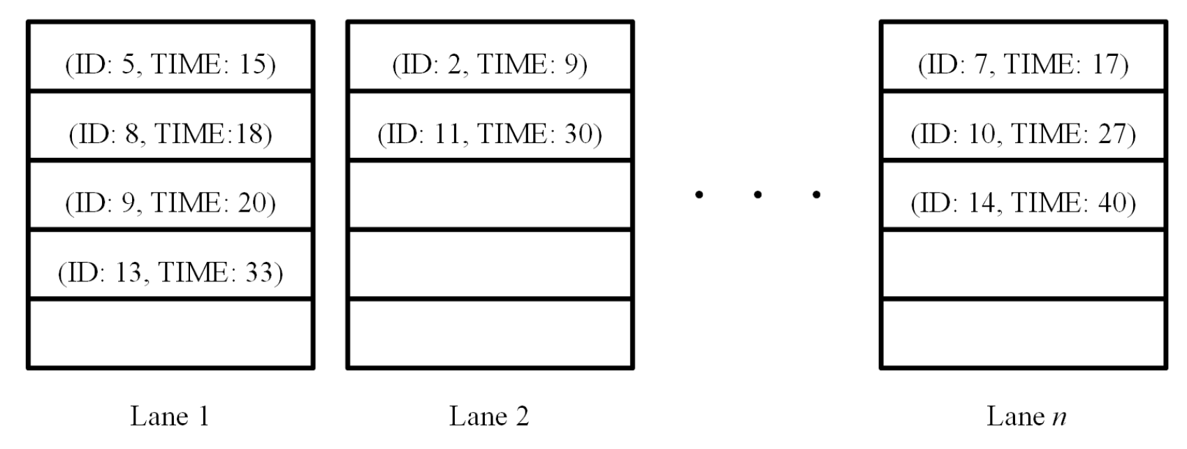
Table 3 specifies the parameters used in this experiment. In each training epoch, we simulate for 200 s by using a high inflow rate (100 vehicle arrivals per minute). The capacity of memory which stores the experience sequence set ( s t , a t , r t + 1 , s t + 1 ) is a set of 100,000 where s t is the state of traffic environment at time t, a t is the action selected by agent at time t, r t + 1 is the reward received at time t and s t + 1 is the state of traffic environment at time t + 1 . The batch size used in training DRLAIM is 64, and the value of the discount factor used in calculating the action value function is 0.99.
We calculate the value of ϵ , shown in Equation (9), which is used to determine the probability for an agent to choose an action:
ϵ = ϵ min + ( ϵ max ϵ min ) × e 0.02 × s t e p s
where
  • ϵ min is the minimum value of ϵ which is taken as 0.01 in this work.
  • ϵ min is the maximum value of ϵ which is taken as 1 in this work.
  • s t e p s is the the current training epoch.
As the value of s t e p s increases, the value of ϵ will decrease from 1 to 0.01. The reason we use Equation (9) to decrease the value of ϵ gradually is as follows. At the beginning of training, the agent will randomly choose an action to explore the environment because the DRLAIM has not yet learned anything; thus, we cannot use it to predict the best action. As the training proceeds, we can gradually increase the ratio to use the trained DRLAIM to predict actions. We now introduce two performance indicators to evaluate the performance of our model.
Average Queue Length (AQL): If the velocity of a vehicle in an incoming lane is smaller than 0.1 m/s, then the vehicle is considered to be in a queue. The total queue length is computed by adding the queue lengths of all incoming lanes. We will calculate the total queue length once every 0.1 s.
Average Waiting Time (AWT): The time that a vehicle is waiting in a queue is called waiting time. We will calculate the waiting time of all vehicles and record the number of vehicles waiting over the whole simulation. The summation of the waiting time of vehicles divided by the number of waiting vehicles is called the average waiting time (AWT).
Table 4 and Table 5 show the average performance between first 10 epochs and the last 10 epochs of the 8 reward functions. We can see that the average performance of the last 10 training epochs among the 8 reward functions outperforms that of first 10 training epochs which means our DRLAIM model did learn a good policy after training. Table 6 shows the average performance over another 10 simulations for the 8 reward functions. We can see that the average performance of reward function 7 outperforms other reward functions. According to this simulation result, we will use reward function 7 to do a further evaluation by using different training epochs and different action time steps.
The performance of the proposed DRLAIM while training is shown in Figure 8, Figure 9 and Figure 10. Figure 8, Figure 9 and 
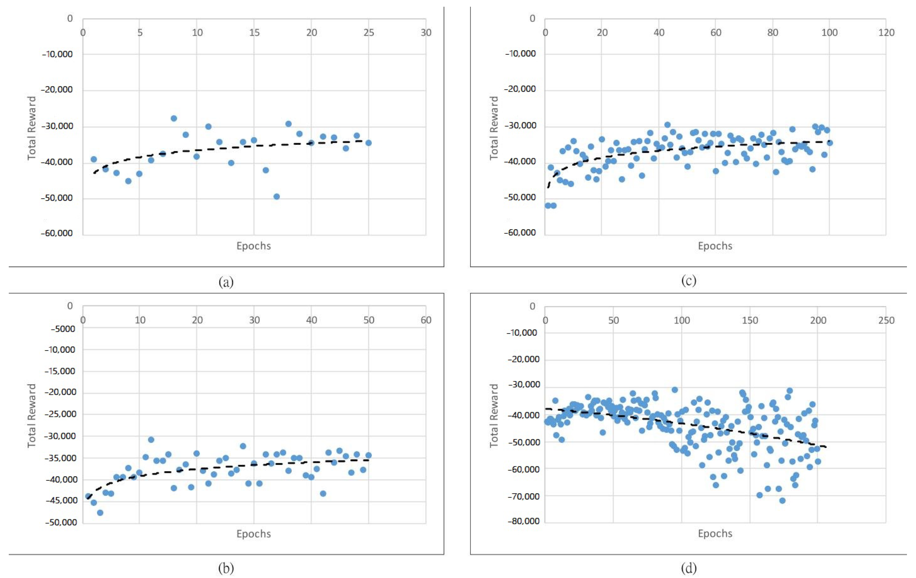
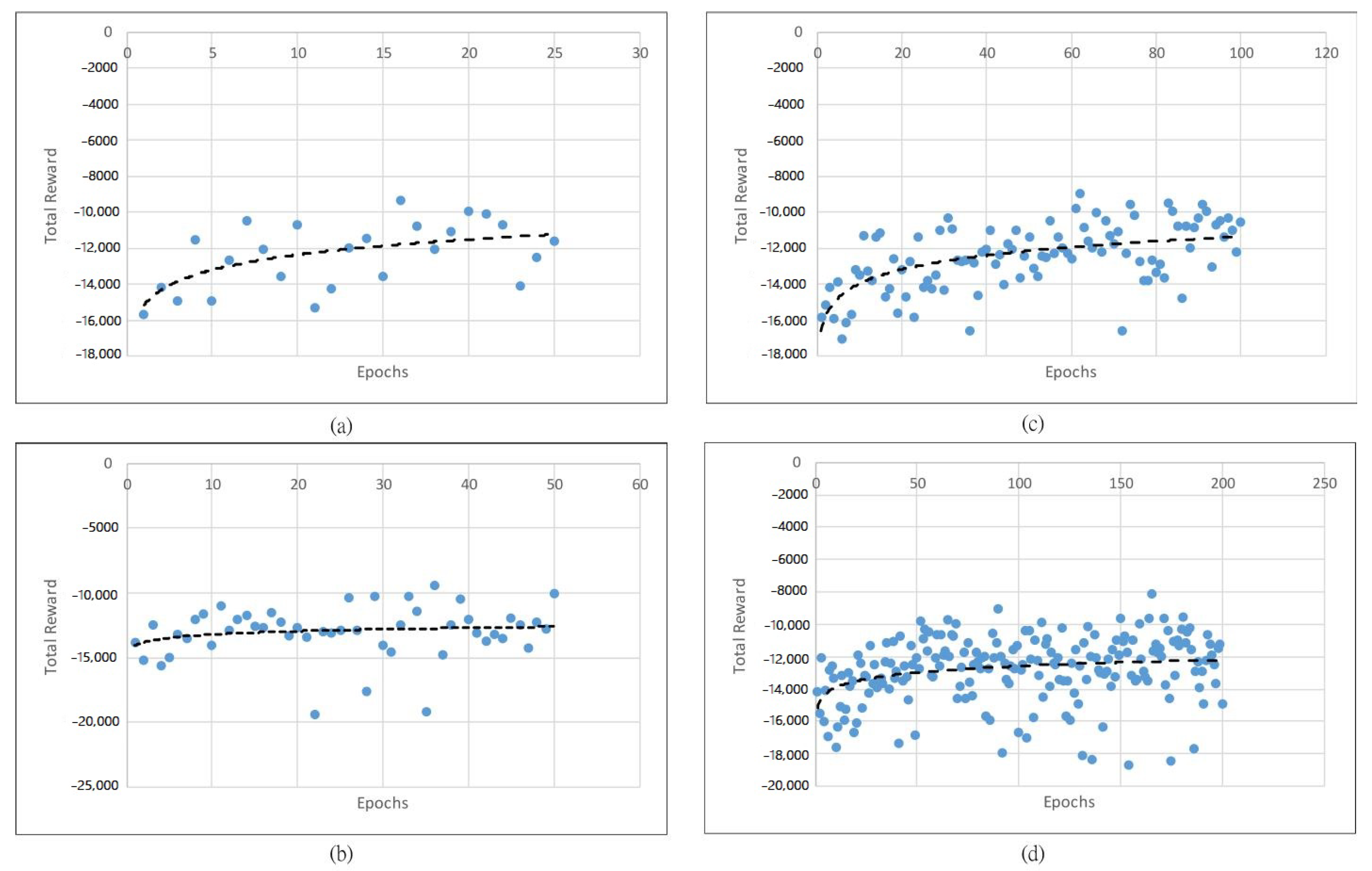
Figure 10 show the value of the total reward obtained after training the model by using 25, 50, and 100 and 200 training epochs and 0.2, 0.5, and 1 s action time steps, respectively. The X-axis represents the epochs, and the Y-axis represents the total reward in Figure 8.
The total reward generated by DRLAIM is trained with 25 epochs, as shown in Figure 8a, and it gives the total reward at 25 epochs of 34,357.28 . Then we have increased the epoch as 50, which is depicted in Figure 8b, which gives the total reward as 34,397.38 , which has higher negative values at 25 epochs; thus we have again increased the epochs to 100 and recorded the total reward, which is 34,303.90 . From Figure 8c, we can understand that during the training of the DRLAIM model at 100 epochs, we are getting lower negative reward values than at 25, 50, and 200 epochs. We can conclude that even if the number of epochs increases, the model will not give good performances. We need to decide the optimal epochs for the training model. We can see that except for the model trained with 100 epochs and time step 0.2 s, the total reward increases gradually as the number of epochs increases. 
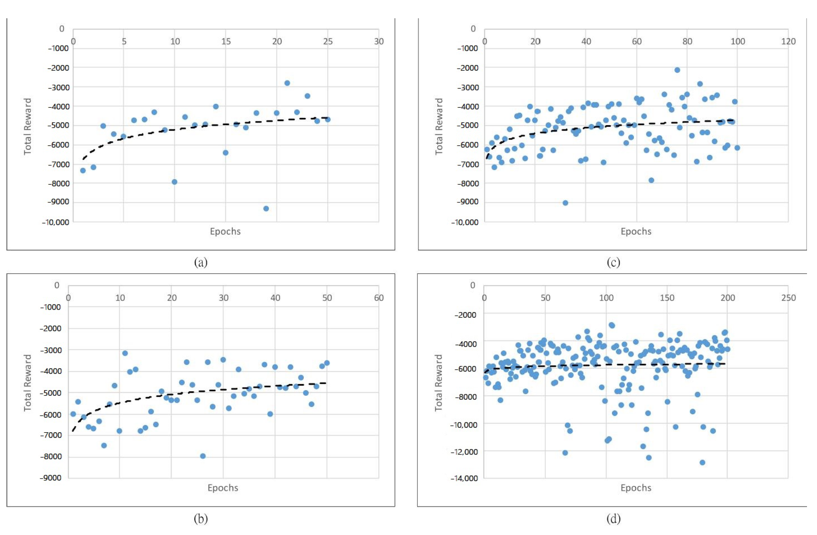
Figure 9 shows a total reward value of 25, 50, 100, and 200 epochs during time step value 0.5From Figure 9, we can understand that our model performs well in the 50-epoch range. When we want to deploy the model in the real-time environment, we need to consider the average queue length, average waiting time and throughput with different time step values, such as 0.1, 0.2 and 1 s. Table 7, Table 8 and Table 9 show the average performance over 10 simulations for the models trained with 4 different number of epochs by using 3 different action time steps. We can see that in-terms of reward performance, the trained model using 100 epochs and a time step of 0.2 s is best.
Figure 11, Figure 12, Figure 13 and 
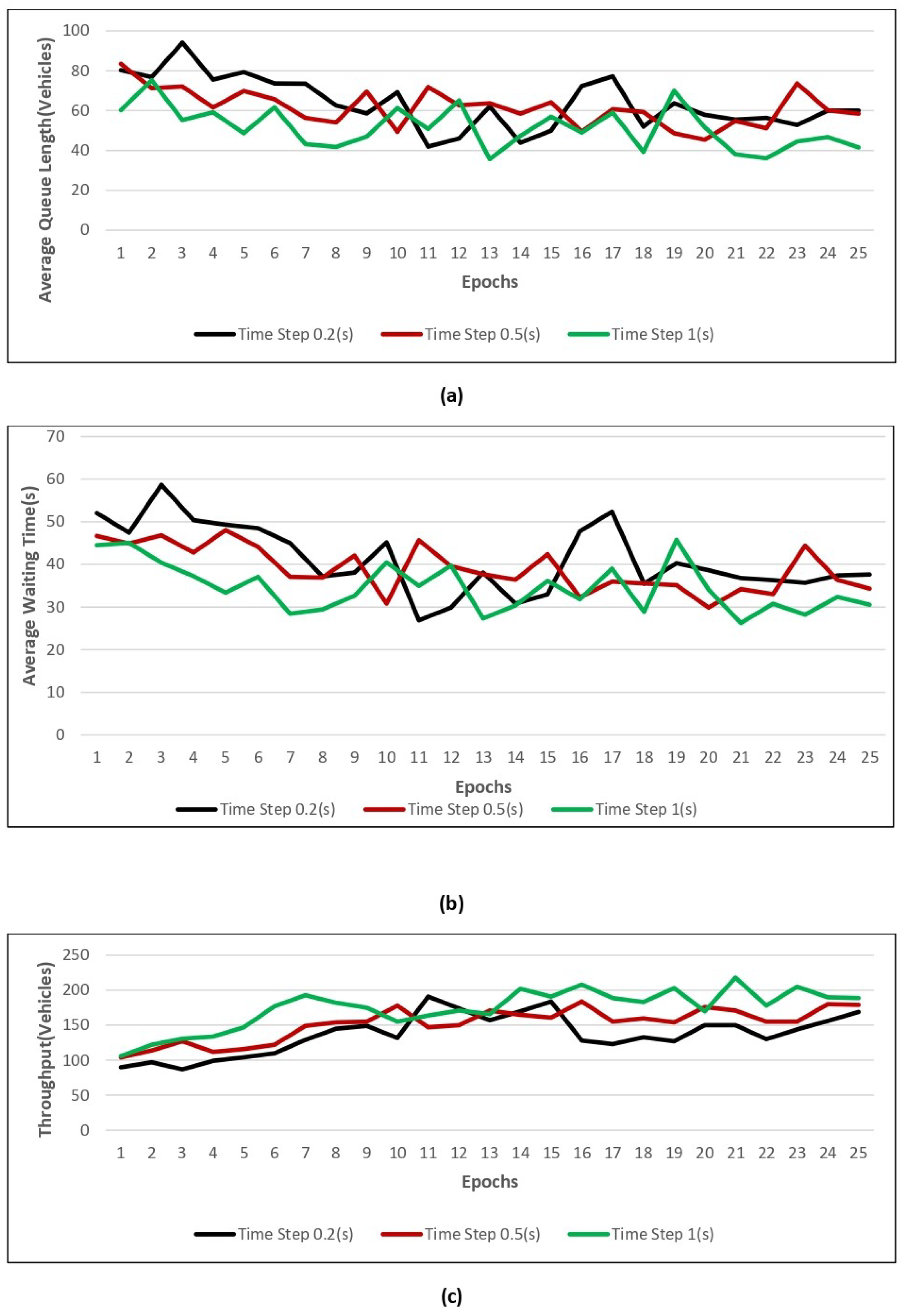
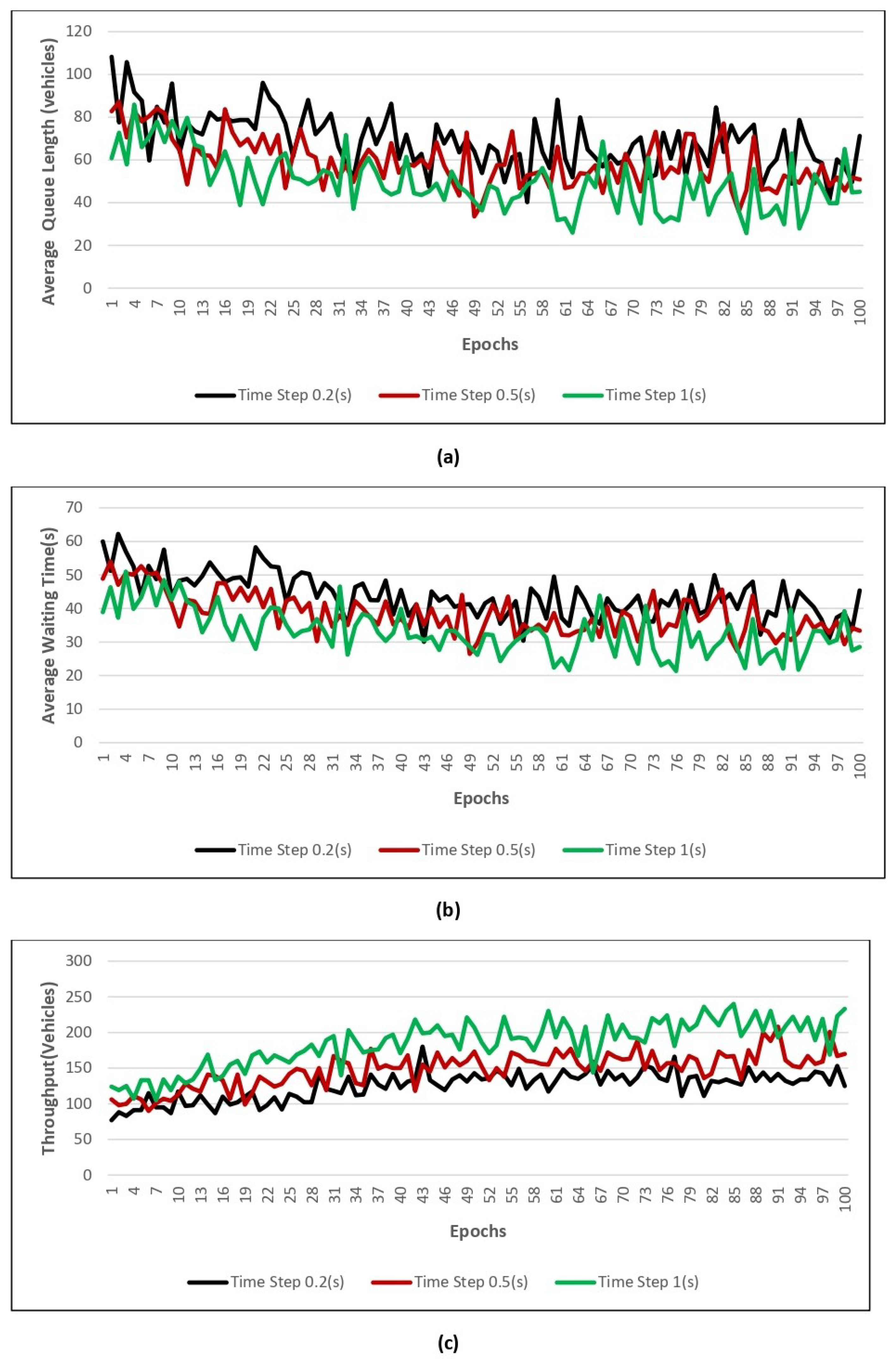
Figure 14 show the value of the three performance indicators introduced above, namely AQL, AWT, and throughput, for models trained with four different numbers of epochs using three different action time steps. Figure 11 shows the performance results when training with 0.2, 0.5, and 1 time steps by using 25 epochs. From Figure 11, we can see that it outperforms the model in terms of average waiting time, queue length, and throughput during the time step value 1. However, it is not giving good performances regarding average queue length, average waiting time, and throughput during the time step value of 1 s when the epoch is 50. 
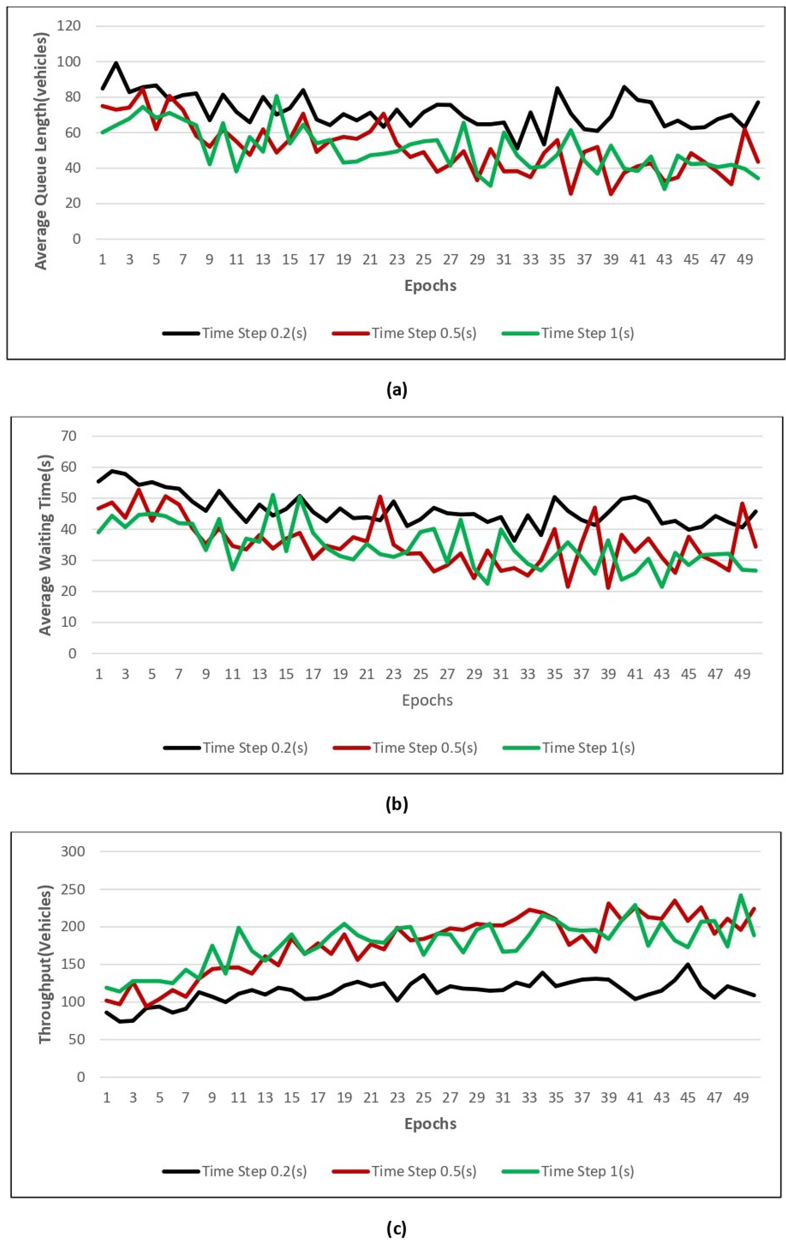
Figure 12 shows the performance results while training with 0.2, 0.5, and 1 time steps and using 50 epochs. From Figure 12, we can understand that 50 epochs give good performances in terms of average queue length, average waiting time, and throughput during the time step value of 0.2 s.
Figure 13 shows the performance results while training with 0.2, 0.5 and 1 time steps using 100 epochs. We can understand that AWT, AVL and throughput are during the time step value 1, which is depicted in the Figure 13. 
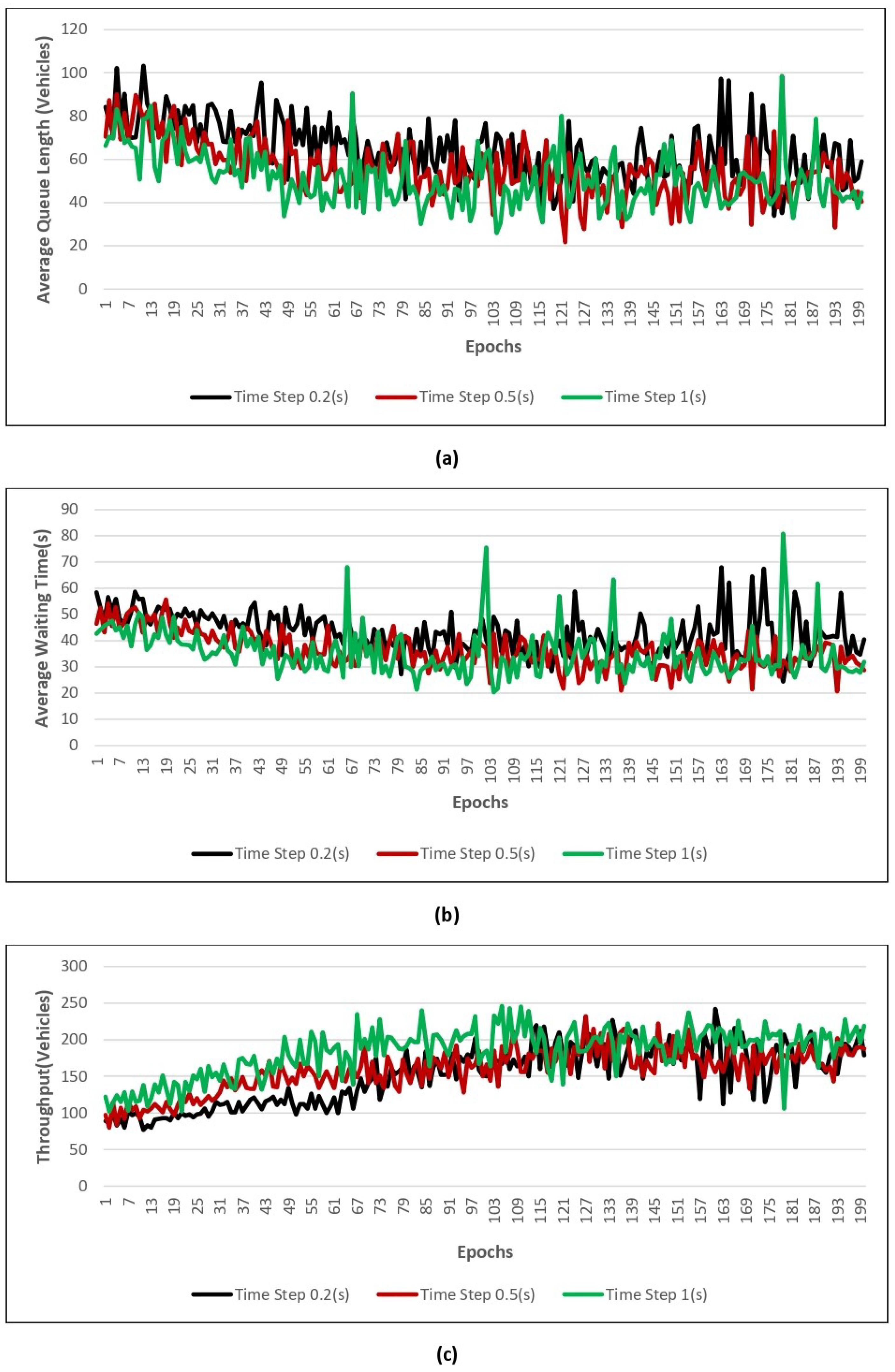
Figure 14 shows the performance results while training with 0.2, 0.5, and 1 time step and using 200 epochs. From Figure 14 we can conclude that 200 epochs give good performances in terms of average queue length, average waiting time, and throughput during the time step value of 1 s. Therefore, we need to decide on time steps and a number of epochs to deploy the model in the real-time environment. For example Figure 13, we can understand that the proposed model performs well in terms of all the parameters during the time step value 1.
To find a better model, we computed the sum of the value of all the parameters and compared them with each other. Table 7, Table 8 and Table 9 show the average performance over ten simulations for the models trained with 4 different numbers of epochs using 3 different action time steps. We can see that the overall performance of the trained model using 50 epochs and time step 0.5 s is best.

4.3.2. Comparison with FFS Method

The fast first service (FFS) method is compared with our model by using a model trained over 50 epochs with a 0.5-s [5]. We use the same parameters as shown in Table 1 and use the four different inflow rates, including 25, 50, 75, and 100 vehicles per minute, to simulate for 200 s. We have tested each model 10 times for each four inflow rate. Table 10 depicts results. When compared to the FFS method, our model outperforms in terms of average waiting time and average queue length, as well as throughput. We think that the waiting time consideration in the suggested reward function, which results in a much more fair action selection strategy, causes the reduction in AWT by DRLAIM.

5. Conclusions

In this study, we suggested an autonomous intersection management system (DRLAIM) inspired by deep reinforcement learning to develop an intersection-crossing strategy. DRLAIM establishes accelerated control of every vehicle, ensuring safety by preventing collisions. We examined eight different reward functions, and the experiment results indicate that the intersection control model with reward function 7 had an 83 percent improvement in throughput. In the future, we can consider simulating different types of intersections, such as roundabouts, to assess the suitability of DRLAIM for other types of intersections. Furthermore, we can consider using an environment with multiple intersections to simulate the interactions between different intersections, i.e., whether the decision made for one intersection would affect adjacent intersections or not. Finally, we can design a strategy that can be applied to autonomous vehicles and incorporate pedestrians and cyclists in an intersection.

Author Contributions

Conceptualization, P.-A.H.; methodology, W.-L.C.; formal analysis, P.K.; investigation, P.K.; data curation, W.-L.C.; writing—review and editing, P.K. and P.-A.H.; supervision, P.-A.H. All authors have read and agreed to the published version of the manuscript..

Funding

This research received no external funding.

Institutional Review Board Statement

Not applicable.

Informed Consent Statement

Not applicable.

Data Availability Statement

Not applicable.

Conflicts of Interest

The authors declare no conflict of interest.

References

  1. CARE–Community Database on Accidents on the Roads in Europe. Available online: https://road-safety.transport.ec.europa.eu/system/files/2021-07/asr2020.pdf (accessed on 21 July 2022).
  2. Antonio, G.P.; Maria-Dolores, C. AIM5LA: A Latency-Aware Deep Reinforcement Learning-Based Autonomous Intersection Management System for 5G Communication Networks. Sensors 2022, 22, 2217. [Google Scholar] [CrossRef] [PubMed]
  3. Chen, W.L.; Lee, K.H.; Hsiung, P.A. Intersection crossing for autonomous vehicles based on deep reinforcement learning. In Proceedings of the 2019 IEEE International Conference on Consumer Electronics-Taiwan (ICCE-TW), IEEE, Yilan, Taiwan, 20–22 May 2019; pp. 1–2. [Google Scholar]
  4. Ganesh, A.H.; Xu, B. A review of reinforcement learning based energy management systems for electrified powertrains: Progress, challenge, and potential solution. Renew. Sustain. Energy Rev. 2022, 154, 111833. [Google Scholar] [CrossRef]
  5. Qian, X.; Altché, F.; Grégoire, J.; de La Fortelle, A. Autonomous Intersection Management systems: Criteria, Implementation and Evaluation. IET Intell. Transp. Syst. 2017, 11, 182–189. [Google Scholar] [CrossRef]
  6. Saraoglu, M.; Pintscher, J.; Janschek, K. Designing a Safe Intersection Management Algorithm using Formal Methods. IFAC-PapersOnLine 2022, 55, 22–27. [Google Scholar] [CrossRef]
  7. Wu, J.; Qu, X. Intersection control with connected and automated vehicles: A review. J. Intell. Connect. Veh. 2022. ahead-of-print. [Google Scholar]
  8. Zamfirache, I.A.; Precup, R.E.; Roman, R.C.; Petriu, E.M. Reinforcement Learning-based control using Q-learning and gravitational search algorithm with experimental validation on a nonlinear servo system. Inf. Sci. 2022, 583, 99–120. [Google Scholar] [CrossRef]
  9. Sutton, R.S.; Barto, A.G. Reinforcement Learning: An Introduction; MIT Press: Cambridge, MA, USA, 2017; p. 2. [Google Scholar]
  10. Velasco-Hernandez, G.; Caicedo-Bravo, E.; Barry, J.; Walsh, J. Intersection management systems and internet of things: A review. In Proceedings of the 2020 IEEE 16th International Conference on Intelligent Computer Communication and Processing (ICCP), IEEE, Cluj-Napoca, Romania, 3–5 September 2020; pp. 439–445. [Google Scholar]
  11. Shaaban, M.E.; Shehata, O.M.; Morgan, E.I. Performance Analysis of Centralized Vs Decentralized Control of an Intelligent Autonomous Intersection. In Proceedings of the 2022 IEEE International Conference on Smart Mobility (SM), IEEE, Chengdu, China, 22–24 October 2022; pp. 8–13. [Google Scholar]
  12. González, C.L.; Delgado, S.L.; Alberola, J.M.; Niño, L.F.; Julián, V. Toward Autonomous and Distributed Intersection Management with Emergency Vehicles. Electronics 2022, 11, 1089. [Google Scholar] [CrossRef]
  13. Shu, H.; Liu, T.; Mu, X.; Cao, D. Driving tasks transfer using deep reinforcement learning for decision-making of autonomous vehicles in unsignalized intersection. IEEE Trans. Veh. Technol. 2021, 71, 41–52. [Google Scholar] [CrossRef]
  14. Liu, B.; Shi, Q.; Song, Z.; El Kamel, A. Trajectory planning for autonomous intersection management of connected vehicles. Simul. Model. Pract. Theory 2019, 90, 16–30. [Google Scholar] [CrossRef]
  15. Silva, V.; Siebra, C.; Subramanian, A. Intersections management for autonomous vehicles: A heuristic approach. J. Heuristics 2022, 28, 1–21. [Google Scholar] [CrossRef]
  16. Mondal, M.; Rehena, Z. Priority-Based Adaptive Traffic Signal Control System for Smart Cities. SN Comput. Sci. 2022, 3, 1–11. [Google Scholar] [CrossRef]
  17. Qiao, J.; Zhang, D.; Jonge, D.d. Priority-Based Traffic Management Protocols for Autonomous Vehicles on Road Networks. In Proceedings of the Australasian Joint Conference on Artificial Intelligence, Sydney, Australia, 2–4 February 2022; Springer: Cham, Switzerland, 2022; pp. 240–253. [Google Scholar]
  18. Grégoire, J.; Bonnabel, S.; Fortelle, A.D.L. Priority-Based Coordination of Robots. Available online: https://hal.archives-ouvertes.fr/hal-00828976/ (accessed on 21 July 2022).
  19. Davis, C.W.; Giabbanelli, P.J.; Jetter, A.J. The intersection of agent based models and fuzzy cognitive maps: A review of an emerging hybrid modeling practice. In Proceedings of the 2019 Winter Simulation Conference (WSC), Washington, MD, USA, 8–12 December 2019; pp. 1292–1303. [Google Scholar]
  20. Prabuchandran, K.J.; Hemanth Kumar, A.N.; Bhatnagar, S. Decentralized Learning for Traffic Signal Control. In Proceedings of the 7th International Conference on Communication Systems and Networks (COMSNETS), Bangalore, India, 6–10 January 2015; pp. 1–6. [Google Scholar]
  21. Jin, J.; Ma, X. Adaptive Group-Based Signal Control Using Reinforcement Learning with Eligibility Traces. In Proceedings of the IEEE 18th International Conference on Intelligent Transportation Systems, Gran Canaria, Spain, 15–18 September 2015; pp. 2412–2417. [Google Scholar]
  22. Kusari, A.; Li, P.; Yang, H.; Punshi, N.; Rasulis, M.; Bogard, S.; LeBlanc, D.J. Enhancing SUMO simulator for simulation based testing and validation of autonomous vehicles. In Proceedings of the 2022 IEEE Intelligent Vehicles Symposium (IV), Aachen, Germany, 4–9 June 2022; pp. 829–835. [Google Scholar]
Figure 1. Combination of traffic phases at intersection.
Algorithms 15 00326 g001
Figure 2. Proposed system architecture.
Algorithms 15 00326 g002
Figure 3. The architecture of queue.
Algorithms 15 00326 g003
Figure 4. An example of interaction between two vehicles, where vehicle i has priority over vehicle j. (a) Trajectories of vehicle i and vehicle j have a possible collision. (b) Trajectories of vehicle i and vehicle j have no collision.
Algorithms 15 00326 g004
Figure 5. An example of selecting different actions. (a) Agent selects an action to let vehicles in a specific lane to pass. (b) Agent selects the action to let all vehicles that have sent requests to pass.
Algorithms 15 00326 g005
Figure 6. Flow of intersection control policy.
Algorithms 15 00326 g006
Figure 7. Intersection model used in our experiments.
Algorithms 15 00326 g007
Figure 8. Total reward while training by using action time step 0.2 s with epochs (a) 25, (b) 50, (c) 100, and (d) 200.
Algorithms 15 00326 g008
Figure 9. Total reward while training using action time step 0.5 s with epochs (a) 25, (b) 50, (c) 100, and (d) 200.
Algorithms 15 00326 g009
Figure 10. Total reward while training using action time step 1 s with epochs (a) 25 (b) 50 (c) 100 (d) 200.
Algorithms 15 00326 g010
Figure 11. Performance results while training with three action time steps and using 25 epochs. (a) AQL. (b) AWT. (c) Throughput.
Algorithms 15 00326 g011
Figure 12. Performance results while training with three action time steps and using 50 epochs. (a) AQL. (b) AWT. (c) Throughput.
Algorithms 15 00326 g012
Figure 13. Performance results while training with three action time steps using 100 epochs. (a) AQL. (b) AWT. (c) Throughput.
Algorithms 15 00326 g013
Figure 14. Performance results while training with three action time steps using 200 epochs. (a) AQL. (b) AWT. (c) Throughput.
Algorithms 15 00326 g014
Table 1. System parameters.
ParameterValue
Car length5 m
Cooperative zone length50 m
Maximum velocity10 m/s
Maximum accelerate4 m/s 2
Minimum accelerate−5 m/s 2
Brake-safe control time step0.1 s
Table 2. Combination of reward functions used for training.
Numbering of Reward FunctionFormula of Reward Function
1 r = r q
2 r = max i w t + 1 i
3 r = r t h
4 r = r q max i w t + 1 i
5 r = r q + r t h
6 r = max i w t + 1 i + r t h
7 r = r q max i w t + 1 i + r t h
8if r min q t i > r q t + 1 i : r = 10 , else: r = 10
Table 3. Parameters used in training experiment.
ParameterValue
Simulation length200 s
Inflow rate100 vel/min
Memory capacity100,000 set
Batch size64
Discount factor0.99
Table 4. Comparison of training results among 8 reward functions for AQL and AWT.
Performance IndicatorAQL (Vehicles)AWT (s)
Compared with First 10 Epochs Last 10 Epochs First 10 Epochs Last 10 Epochs
Reward 168.7555.6343.6336.18
Reward 273.6548.6046.4834.29
Reward 373.9758.3246.0337.03
Reward 472.8254.4245.9636.71
Reward 572.8455.6245.5438.81
Reward 671.0747.1446.2033.86
Reward 769.4441.7544.9233.48
Reward 878.6658.0249.0738.73
Table 5. Comparison of training results among 8 reward functions for throughput.
Performance IndicatorThroughput (Vehicles)
Compared with First 10 Epochs Last 10 Epochs
Reward 1121.4161.3
Reward 2112.7177.1
Reward 3110.9161.9
Reward 4119.0183.7
Reward 5118.8167.1
Reward 6109.9185.4
Reward 7116.8214.1
Reward 8109.8142.5
Table 6. Average performance difference among 8 reward functions.
Reward FunctionAQL (Vehicles)AWT (s)Throughput (Vehicles)
151.4634.67152.5
256.2737.61176.7
360.3138.68141.5
444.0233.70202.4
558.5936.83159.7
653.2434.18187.8
742.8331.71211.3
858.3936.95148.9
Table 7. Average performance of model trained with different number of epochs using action time step 0.2 s.
EpochsPerformance IndicatorTotal RewardAQL (Vehicles)AWT (s)Throughput (Vehicles)
25−36,076.369.8944.12125.1
50−37,373.772.0445.69116.8
100−33,816.063.8840.44150.3
200−50,636.063.7944.57144.5
Table 8. Average performance of model trained with different number of epochs using action time step 0.5 s.
EpochsPerformance IndicatorTotal RewardAQL (Vehicles)AWT (s)Throughput (Vehicles)
25 −11,711.552.1234.45168.3
50−10,239.042.8331.71211.3
100−10,443.050.6933.13167.3
200−12,484.463.7944.57176.5
Table 9. Average performance of model trained with different number of epochs using action time step 1 s.
EpochsPerformance IndicatorTotal RewardAQL (Vehicles)AWT (s)Throughput (Vehicles)
25−4839.845.3729.76197.3
50−5115.445.5731.67191.6
100−5669.144.6931.48201.2
200−6524.550.1137.72189.5
Table 10. Comparison with FFS method.
Inflow Rate (Vehicles/min)100755025
Method DRLAIM FFS DRLAIM FFS DRLAIM FFS DRLAIM FFS
AQL (vehicles)46.0346.0725.8021.7313.127.755.790.63
AWT (s)38.7739.2730.8434.3724.9426.8823.567.74
Throughput (vehicles)211.70222.00180.10197.20126.30148.4073.5079.10
Publisher’s Note: MDPI stays neutral with regard to jurisdictional claims in published maps and institutional affiliations.

