Fed-DeepONet: Stochastic Gradient-Based Federated Training of Deep Operator Networks

Abstract

The Deep Operator Network (DeepONet) framework is a different class of neural network architecture that one trains to learn nonlinear operators, i.e., mappings between infinite-dimensional spaces. Traditionally, DeepONets are trained using a centralized strategy that requires transferring the training data to a centralized location. Such a strategy, however, limits our ability to secure data privacy or use high-performance distributed/parallel computing platforms. To alleviate such limitations, in this paper, we study the federated training of DeepONets for the first time. That is, we develop a framework, which we refer to as Fed-DeepONet, that allows multiple clients to train DeepONets collaboratively under the coordination of a centralized server. To achieve Fed-DeepONets, we propose an efficient stochastic gradient-based algorithm that enables the distributed optimization of the DeepONet parameters by averaging first-order estimates of the DeepONet loss gradient. Then, to accelerate the training convergence of Fed-DeepONets, we propose a moment-enhanced (i.e., adaptive) stochastic gradient-based strategy. Finally, we verify the performance of Fed-DeepONet by learning, for different configurations of the number of clients and fractions of available clients, (i) the solution operator of a gravity pendulum and (ii) the dynamic response of a parametric library of pendulums.

1. Introduction

High-fidelity numerical methods have revolutionized how we predict and simulate complex engineering dynamical systems, such as power grids, robotics, and communication networks. However, these methods become prohibitively expensive as the complexity of the system increases. Furthermore, the elevated computational cost of these methods has prevented their use for tasks that require multiple forward simulations, e.g., control, optimization, and uncertainty quantification. Thus, it is imperative to develop faster numerical solvers to tackle the most complex problems in science and engineering.

1.1. Previous Works

Deep learning [1] has radically advanced the state-of-the-art in areas such as computer vision and natural language processing and promises to deliver faster tools for predicting and simulating complex dynamical systems. As a result, a recent wave of novel works has developed neural-network-based surrogates to replace current numerical simulation methods. These neural-network-based surrogates (i) learn to predict the future states of the system based on the current state [2,3,4], (ii) encode the underlying physics equations during training [5], and (iii) identify sparse representations of the underlying dynamic equations from streams of data [6,7,8]. However, most of these neural surrogate models require retraining when the system experiences new (i) operating conditions, (ii) inputs, or (iii) parametric realizations. These drawbacks have limited the application of neural networks to game-changing technologies such as digital twins [9].

To tackle the above drawbacks, in the seminal paper [10], Lu et al. built on the universal approximation theorem for nonlinear operators [11] to design a Deep Operator Network (DeepONet) framework. DeepONet is trained using gradient-based optimization methods (e.g., Adam [12]) to approximate a mapping between two infinite-dimensional spaces, e.g., the solution operator of a complex dynamical system. Compared to more traditional neural networks [1], the proposed DeepONet effectively learns such a complex mapping using streams of scattered data and exhibits enhanced generalization capabilities. These capabilities have been demonstrated in applications, including multi-physics problems [13], power systems [14], and control systems [15]. However, the gradient-based training for DeepONet requires transferring all the training data to a centralized location for processing. Such a practice may prevent using DeepONet for applications where (i) the data are collected from multiple clients whose security must be protected or (ii) multiple distributed/parallel high-performances are available for training. Examples of such applications include the development of digital twins for predicting (i) household electrical consumption, (ii) vehicular traffic flow, or (iii) the transmission dynamics of contagious diseases (e.g., COVID-19).

To circumvent the data security properties and allow the distributed training of neural networks, McMahan et al. [16] introduced Federated Learning as a newly developed learning framework with appealing properties. Federated learning (i) allows multiple clients to train a collaborative learning model under the coordination of a centralized server and (ii) keeps the training data on local clients where data privacy, security, and access rights are a matter of vital interest. Keeping the data at local clients protects data privacy, and coordinating local updates with a centralized server saves significant data transfer volume, which yields beneficial communication cost reduction. The standard formulation of federated learning is a distributed optimization framework that tackles communication costs and client robustness [17]. Central to the formulation is communication efficiency, which directly motivates the most well-known efficient communication algorithm in federated learning: the federated averaging (FedAvg) algorithm [16]. FedAvg has been studied under realistic scenarios in [18,19,20]. Furthermore, many works have provided convergence proofs of the algorithm within the field of optimization [21,22,23,24].

1.2. Our Work

In this paper, we aim to develop, for the first time, a federated [16] training framework for Deep Operator Networks, which we refer to as Fed-DeepONet. To this end, we propose an efficient stochastic gradient-based algorithm that enables the distributed optimization of the DeepONet parameters by averaging first-order estimates of the DeepONet loss gradient. Then, we propose a moment-enhanced (i.e., adaptive) stochastic gradient-based strategy that increases the speed of training convergence of Fed-DeepONet, i.e., an Adaptive Fed-DeepONet framework. Finally, as a proof of concept, we verify the performance of Fed-DeepONet using two experiments with different configurations of the number of clients and different fractions of available clients. The experiments aim at training Fed-DeepONets for learning (i) the solution operator of a pendulum and (ii) the dynamic response of a parametric library of pendulums.

We remark that compared to the traditional federated training of neural networks (FedAvg), the proposed Fed-DeepONet algorithms target the more complex problem of approximating, in a distributed/federated manner, the infinite-dimensional response of nonlinear operators. As a result, we can use a trained Fed-DeepONet to tackle complex engineering and scientific computing tasks (e.g., learning digital twins or materials science discovery). These tasks are inherently infinite-dimensional, and we can model them as input-output nonlinear operators. For these infinite-dimensional tasks, however, the traditional FedAvg for training neural networks, which only approximates mappings between finite-dimensional spaces in a distributed manner, will fail unless the designer makes stringent/unrealistic assumptions (e.g., computes the output response for only a fixed parameter value or a single initial condition) and uses enormous datasets. In addition, we will demonstrate in our numerical experiments that Fed-DeepONet significantly reduces the generalization error, similar to the centralized DeepONet. This generalization capability makes the proposed Fed-DeepONet framework more robust to non-independent and identically distributed scenarios than the traditional FedAvg training strategy for deep neural networks. Finally, the proposed Fed-DeepONet has the following unique feature: It can effectively tackle data heterogeneity problems in the output functional space (i.e., when the parametric responses of the clients are different) by learning all possible parametric responses.

We organize the rest of the paper as follows. Section 2 provides a brief review of the centralized training of Deep Operator Networks (DeepONet). Section 3 proposes gradient-based and moment-enhanced (i.e., adaptive) algorithms for the federated training of DeepONets (Fed-DeepONet). In Section 4, we demonstrate the effectiveness of the proposed Fed-DeepONet by learning (i) the solution operator of a gravity pendulum and (ii) a library of pendulums. Finally, Section 5 discusses our results and limitations, and Section 6 concludes the paper.

2. Background Information

Let us consider the problem of approximating a nonlinear operator G from data. Operator G maps two infinite-dimensional spaces, i.e., it maps an input function u to an output function $G\left(u\right)$. The input u may (i) represent, for example, a forcing term, a control input, or a parametric realization and (ii) belong to the space of continuous or measurable functions. Let $y\in Y$ denote a query location within the output domain Y. Then, our goal in this paper is to employ a Deep Operator Network (DeepONet) $G_{\theta }$ with trainable parameters $\theta \in {\mathbb{R}}^s$ to learn from data nonlinear operators $G\left(u\right)\left(y\right)$ at query locations $y\in Y$.

As a proof of concept, in our numerical experiments (see Section 4), we will study the problem of learning the solution operator G arising when solving a complex dynamical system described via the initial value problem (IVP):

$$\begin{array}{c}\begin{array}{cc}\hfill \frac{d}{dt}x\left(t\right)& =f\left(x\right(t),u(t);\lambda ),t\in [0,T],\hfill \\ \hfill x\left(0\right)& =x_0,\hfill \end{array}\end{array}$$

(1)

where $x\left(t\right)\in {\mathbb{R}}^d$ is the vector-valued state function, $u\left(t\right)\in {\mathbb{R}}^m$ is an input function, $\lambda \in {\mathbb{R}}^p$ is a parameter realization, and $f:{\mathbb{R}}^d\times {\mathbb{R}}^m\to {\mathbb{R}}^d$ is the unknown vector field. The solution operator of (1), i.e., $G:u\mapsto G\left(u\right)\equiv x$, is given by

$$\begin{array}{c}\hfill G\left(u\right)\left(t\right)=x_0+{\int }_0^{t}f(G\left(u\right)\left(s\right),u\left(s\right);\lambda )ds,t\in [0,T].\end{array}$$

(2)

Let us now review the traditional centralized strategy for training DeepONets.

Centralized Training of DeepONets

To approximate G, DeepONet [10] employs a neural network architecture (see Figure 1) that uses two subnetworks: the Trunk network and the Branch network.

The Branch network processes the input function u information. Let $(x_1,\dots ,x_m)$ be the collection of m interpolation points $(x_1,\dots ,x_m)$ (known as sensors in the original paper [10]) that enable us to discretize/encode the input function, i.e., $u_m:=(u\left(x_1\right),\dots ,u\left(x_m\right))$. The Branch network maps this discretized input $u_m$ to a vector of trainable coefficients $b\in {\mathbb{R}}^q$. On the other hand, the Trunk network processes the query location $y\in Y$. To this end, the Trunk network maps the query location y to the following collection of trainable basis functions:

$$\phi :=({\phi }_1\left(y\right),\dots ,{\phi }_q\left(y\right))\in {\mathbb{R}}^q.$$

The output of DeepONet is then computed by fusing the trainable coefficients b with the trainable basis functions $\phi$ using the following dot product:

$$\begin{array}{c}\hfill G_{\theta }\left(u_m\right)\left(y\right):=\sum _{i=1}^q{b}_i·{\phi }_i\left(y\right).\end{array}$$

(3)

The traditional DeepONet $G_{\theta }$ centralized training strategy collects the following training dataset from possibly distributed locations:

$${\mathcal{D}}_{\mathrm{cent}}:={\left\{u_m^{(k)},y^{(k)},G(u_m^{(k)})(y^{(k)})\right\}}_{k=1}^N.$$

Then, at a centralized location, one trains the DeepONet parameter $\theta$ by minimizing (e.g., using the gradient-based Adam [12] algorithm) the following mean squared loss function:

$$\mathcal{L}(\theta )=\frac{1}{N}\sum _{k=1}^N{∥G_{\theta }(u_m^{(k)})(y^{(k)})-G(u_m^{(k)})(y^{(k)})∥}_2^2$$

over the centralized dataset ${\mathcal{D}}_{\mathrm{cent}}$. Such a centralized training strategy may (i) fail to protect the privacy of distributed clients, e.g., when learning digital twins for engineering applications, or (ii) prevent using high-performance parallel and distributed computing frameworks for scientific computing applications. To alleviate the aforementioned limitations of the centralized strategy, we propose, in the following section, a federated/distributed training strategy for DeepONets, which we refer to as Fed-DeepONet.

3. Federated Deep Operator Networks (Fed-DeepONet)

Let us start this section by describing some mathematical notations from federated learning [17]. We let $\lfloor ·\rfloor$ denote the floor function, and we use ${\parallel ·\parallel }_2$ to denote the standard Euclidean norm. For any given positive integer n, we let $\left[n\right]$ denote the set $\{1,2,\dots ,n\}$. We let C denote the number of clients participating in the federated training of DeepONet and use variable c to describe the clients within the set of clients $\left[C\right]$. For each client $c\in \left[C\right]$, we use ${\mathcal{L}}^c$ and $\nabla {\mathcal{L}}^c$ to denote the c-th client’s corresponding DeepONet loss and gradient of the loss ${\mathcal{L}}^c$. We let $\nabla {\tilde{\mathcal{L}}}^c$ denote the stochastic gradient of ${\mathcal{L}}^c$ computed using the c-th client’s dataset. This stochastic gradient $\nabla {\tilde{\mathcal{L}}}^c$ is an unbiased estimator of the exact gradient $\nabla {\mathcal{L}}^c$ [25]. We also denote $p_c$ as the weight of the c-th client such that $p_c=\frac{n_c}{{\sum }_{i\in \left[C\right]}{n}_i}\in (0,1)$, where $n_c>0$ is the number of data triplets in the c-th client. Let K denote the number of local stochastic gradient updates taken by each client $c\in \left[C\right]$ and let R denote the number of global synchronization events (also known as the number of communication rounds).

To train the proposed Fed-DeepONet, we follow a distributed optimization strategy. For traditional neural networks, this distributed strategy was introduced in [16,18], and it is known as federated averaging (FedAvg). Formally, we aim to solve the following optimization problem:

$$\begin{array}{c}\hfill \underset{\theta \in {\mathbb{R}}^s}{min}\frac{{\sum }_{c=1}^C{\mathcal{L}}^c(\theta )}{{\sum }_{c=1}^C{n}_c}.\end{array}$$

(4)

In the above, ${\mathcal{L}}^c(\theta ):={\sum }_{j=1}^{n_c}\ell \left(\theta ;d_c^{\left(j\right)}\right)$, where $\theta \in {\mathbb{R}}^s$ and $\ell \left(\theta ;d_c^{\left(j\right)}\right)$ is the c-th client’s DeepONet loss function based on $\theta$ and the data triplet $d_c^{\left(j\right)}:=\{u_{m,c}^{\left(j\right)},y_c^{\left(j\right)},G\left(u_{m,c}^{\left(j\right)}\right)\left(y_c^{\left(j\right)}\right)\}$ collected by the c-th client, i.e.,

$$\ell \left(\theta ;d_c^{\left(j\right)}\right)={∥G_{\theta }\left(u_{m,c}^{\left(j\right)}\right)\left(y_c^{\left(j\right)}\right)-G\left(u_{m,c}^{\left(j\right)}\right)\left(y_c^{\left(j\right)}\right)∥}_2^2.$$

Here, we have used the notations $u_{m,c},y_c$ and $G\left(u_{m,c}\right)\left(y_c\right)$ to emphasize that $u_{m,c},y_c$ and $G\left(u_{m,c}\right)\left(y_c\right)$ are, respectively, a discretized input, query location, and solution operator value collected by the c-th client.

The proposed Fed-DeepONet framework can work with independent and identically distributed and non-independent and identically distributed (heterogeneous) data. However, most of the applications we seek for Fed-DeepONet (e.g., learning digital twins, scientific computing, or material discovery) will present some level of data heterogeneity. For example, when the clients’ data presents slightly different properties while sharing some others. To provide a more detailed explanation for the causes of heterogeneous data, let us use the joint probability density function $p_i(\{u_m,y\},G\left(u_m\right)\left(y\right))$ of the i-th client input–output data samples. Observe that we can factorize this joint as $p_i(\{u_m,y\},G\left(u_m\right)\left(y\right))=p_i\left(\{u_m,y\}\right)p_i\left(G\left(u_m\right)\left(y\right)\right|\{u_m,y\})$. Using this factorization, we can establish three causes of heterogeneous data for Fed-DeepONet.

1.

Different input distributions. In this situation, we have $p_i\left(\{u_m,y\}\right)\ne p_j\left(\{u_m,y\}\right)$ and $p_i\left(G\left(u_m\right)\left(y\right)\right|\{u_m,y\})=p_j\left(G\left(u_m\right)\left(y\right)\right|\{u_m,y\})$ for some $i,j\in \left[C\right]$. This situation may occur when learning digital twins for synchronous generators. Suppose all the participating clients have generators with the same parameters and assume the datasets collected by each client are different. For instance, assume most clients have stable trajectories in their datasets, while the rest may have many unstable and disturbance trajectories. Such a situation makes the functional input space of the different clients skewed. However, notice that the output functional space remains the same for all clients. In Section 4.3, we will design a simple experiment that evaluates the performance of Algorithms 1 and 2 to different levels of input distribution heterogeneity.

2.

Different conditional distributions. In this situation, we have the conditional probabilities satisfy $p_i\left(G\left(u_m\right)\left(y\right)\right|\{u_m,y\})\ne p_j\left(G\left(u_m\right)\left(y\right)\right|\{u_m,y\})$ and $p_i\left(\{u_m,y\}\right)=p_j\left(\{u_m,y\}\right)$. For an example within the proposed framework, consider the generator digital twin learning task again. Then an example of this situation is when the clients use the same excitation signals for system identification but have generators with different parameters and responses. This paper will not approach such a situation from a federated learning perspective. Instead, we show, in our experiments (see Section 4.4), that Fed-DeepONet can tackle this heterogeneous data situation by learning all parameter realizations (i.e., a library of digital twins) provided each client has access to the generators’ parameters. If the client does not know the parameters, then one could, for example, keep some of the Branch network parameters private. Such a strategy will control the bias introduced during each synchronization round. We left the details of this strategy for our future work.

3.

Different joint probabilities. In this situation, each client’s input and output functional spaces may have slightly different characteristics. In Section 4.3, we present a simple experiment that aims at testing such a situation.

To train the proposed Fed-DeepONet, we first propose a federated averaging implementation of the stochastic gradient descent algorithm. Such an implementation requires us to loop over the following three steps:

1.

Broadcast to clients: The centralized server broadcasts to all the clients $c\in \left[C\right]$ the most up-to-date DeepONet parameters, which we denote as ${\theta }_k$. Here k is an integer variable used to denote the local update number for the c-th client.

2.

Client local updates: For any $c\in \left[C\right]$, the c-th client receives the most up-to-date DeepONet parameters ${\theta }_k$, sets ${\theta }_k^c={\theta }_k$, and then executes $K\ge 1$ local stochastic gradient DeepONet updates over the client’s dataset ${\{d_c^{\left(j\right)}\}}_{j=1}^{n_c}$, i.e.,

$${\gamma }_{k+1}^c={\theta }_k^c-\theta \nabla {\tilde{\mathcal{L}}}^c\left({\theta }_k^c\right),$$

where $\theta$ is the learning rate, and ${\gamma }_{k+1}^c$ is the immediate result of the one-step stochastic gradient update from ${\theta }_k^c$, which implies that ${\theta }_{k+1}^c={\gamma }_{k+1}^c$ if $k+1$ mod K is not equal to zero.

3.

Global synchronization: The centralized server aggregates the local DeepONet parameters into a unique global Fed-DeepONet parameter as follows, ${\theta }_{k+K}:={\sum }_{c\in \left[C\right]}{p}_c{\gamma }_{k+K}^c$.

We provide a summary of the aforementioned training strategy for Fed-DeepONet in Algorithm 1.

Algorithm 1 Federated Deep Operator Network (Fed-DeepONet) learning. Denote by (i) ${\theta }_k^c$ the DeepONet parameters of the c-th client, (ii) ${\gamma }_k^c$ the immediate result from ${\theta }_k^c$ via a local stochastic gradient update, and (iii) $\eta$ the learning rate. A global synchronization round of the DeepONet parameters is executed by the centralized server every K steps. Run the algorithm for R DeepONet synchronization rounds. Formally, for each client $c\in \left[C\right]$, the client locally runs:

$${\gamma }_{k+1}^c={\theta }_k^c-\eta \nabla {\tilde{\mathcal{L}}}^c\left({\theta }_k^c\right),$$ (5) $${\theta }_{k+1}^c=\left\{\begin{array}{c}{\gamma }_{k+1}^c\mathrm{if}k+1\mathrm{mod}K\ne 0\hfill \\ \sum _{c=1}^C{p}_c{\gamma }_{k+1}^c\mathrm{if}k+1\mathrm{mod}K=0.\hfill \end{array}\right.$$ (6)

Theoretically, under some assumptions, one can show (see [21] for details) the convergence of Algorithm 1. In practice, however, not all the clients may be available for federated DeepONet training. To handle this intermittent training scenario, we introduce the set ${\mathcal{A}}_k\subseteq \left[C\right]$, denoting the clients available at global synchronization round k (note that ${\mathcal{A}}_k$ is assumed to be fixed for the next K local updates). Furthermore, we observed that Algorithm 1 might present slow convergence when training Fed-DeepONets (see Section 4.1). One can improve the Fed-DeepONet training convergence by using adaptive (also known as momentum-enhanced) stochastic gradient-based strategies, e.g., Adam [12]. We summarize in Algorithm 2 a federated strategy for handling a variable number of available clients, which collectively trains Fed-DeepONet using a local adaptive stochastic optimization scheme. We call this strategy the Adaptive Fed-DeepONet.

Algorithm 2 Adaptive Federated Deep Operator Network (Adaptive Fed-DeepONet) learning. Denote by (i) ${\theta }_k^c$ the DeepONet parameters of the c-th client, (ii) ${\gamma }_k^c$ the immediate result from ${\theta }_k^c$ via an adaptive local stochastic gradient with momentum update, (iii) $\eta$ the step-size, (iv) ${\beta }_1,{\beta }_2\in [0,1)$ the exponential decay rates for the moment estimates, (v) $m_k^c$ the first-moment vector, (vi) $v_k^c$ the second-moment vector, and (vii) $ϵ\ll 1$ a small positive number introduced to avoid division by zero during Adaptive Fed-DeepONet. A global synchronization round of the DeepONet parameters is executed by the centralized server every K steps. Run the algorithm for R DeepONet synchronization rounds. Formally, for each client $c\in {\mathcal{A}}_k$, the client locally runs:

$$t=k+K\lfloor k/K\rfloor +1,$$ $$m_{k+1}^c=\left\{\begin{array}{c}(1-{\beta }_1)\nabla {\tilde{\mathcal{L}}}^c\left({\theta }_k^c\right)\mathrm{if}k\mathrm{mod}K\ne 0\hfill \\ {\beta }_1{m}_k^c+(1-{\beta }_1)\nabla {\tilde{\mathcal{L}}}^c\left({\theta }_k^c\right)\mathrm{if}k\mathrm{mod}K=0.\hfill \end{array}\right.$$ $$v_{k+1}^c=\left\{\begin{array}{c}(1-{\beta }_2){\left(\nabla {\tilde{\mathcal{L}}}^c\left({\theta }_k^c\right)\right)}^2\mathrm{if}k\mathrm{mod}K\ne 0\hfill \\ {\beta }_2{v}_k^c+(1-{\beta }_2){\left(\nabla {\tilde{\mathcal{L}}}^c\left({\theta }_k^c\right)\right)}^2\mathrm{if}k\mathrm{mod}K=0.\hfill \end{array}\right.$$ $${\widehat{m}}_{k+1}^c=m_{k+1}^c/(1-{\left({\beta }_1\right)}^t)\mathrm{and}{\widehat{v}}_{k+1}^c=v_{k+1}^c/(1-{\left({\beta }_2\right)}^t),$$ $${\gamma }_{k+1}^c={\theta }_k^c-\eta ·\frac{{\widehat{m}}_{k+1}^c}{\left(\sqrt{{\widehat{v}}_{k+1}^c}+ϵ\right)},$$ (7) $${\theta }_{k+1}^c=\left\{\begin{array}{c}{\gamma }_{k+1}^c\mathrm{if}k+1\mathrm{mod}K\ne 0\hfill \\ \sum _{c=1}^C{p}_c{\gamma }_{k+1}^c\mathrm{if}k+1\mathrm{mod}K=0.\hfill \end{array}\right.$$ (8)

4. Numerical Experiments

This section tests the efficacy of the proposed Fed-DeepONet framework. To this end, we use four experiments. In the first experiment (see Section 4.1), we compare the federated training performance of the two proposed algorithms: Algorithm 1 (Fed-DeepONet) and Algorithm 2 (Adaptive Fed-DeepONet). In the second experiment (see Section 4.2), we employ the Adaptive Fed-DeepONet to learn the solution operator of a pendulum. In the third experiment, we verify how the performance of Fed-DeepONet changes when we vary the data heterogeneity. In the final experiment (see Section 4.4), we approximate the dynamic response of a library of pendulums using an Adaptive Fed-DeepONet. Let us start this section by describing the neural networks used for DeepONet, the distributed training dataset, and the metrics used to evaluate Fed-DeepONet.

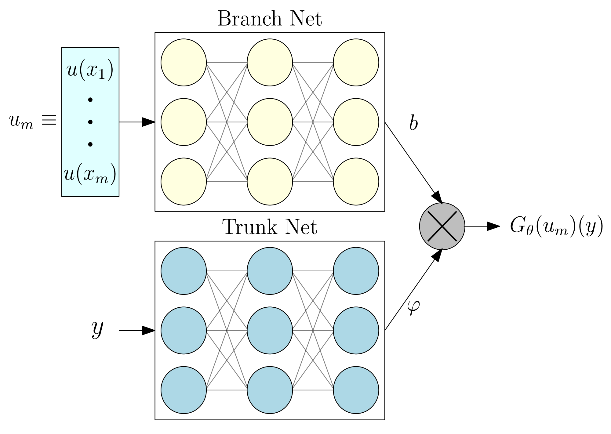
Neural networks. To build the Branch and Trunk networks, we used feed-forward neural networks. For the Branch, we used 1 hidden layer with a width of 50 neurons. Further, the Branch’s input and output layers have, respectively, m (defined later) and 50 neurons. For the Trunk, we also used 1 hidden layer with 50 neurons. The Trunk’s input and output layers have, respectively, 1 and 50 neurons. We obtained these values for the design of the Branch and Trunk networks after employing a simple routine of hyper-parameter optimization. For the activation function, we employed the classical ReLU function. We coded these neural networks in PyTorch and published the code on GitHub.

Training dataset. For each experiment, we collected, using the true operator G, $N=$ 10,000 training data triplets, i.e., ${\{u_m^{\left(k\right)},y^{\left(k\right)},G\left(u_m^{\left(k\right)}\right)\left(y^{\left(k\right)}\right)\}}_{k=1}^N$. Then, we distributed these training data triplets among the C clients without repetition. Note that in these experiments, we used the number of clients C as a parameter to test the performance of Fed-DeepONet.

Metrics. To test the performance of Fed-DeepONet, we computed the $L_2$-relative error between solution trajectories. That is, for a given discretized input $u_m$, we use the trained Fed-DeepONet (denoted as $G_{{\theta }^{*}}$, where ${\theta }^{*}$ is the vector of trained/optimized parameters) to predict the solution trajectory ${\widehat{V}}_{u_m}:=\{G_{{\theta }^{*}}\left(u_m\right)\left(t\right):t\in T_m\}$ at a collection of selected points $T_m\subset [0,T]$. Let $V_{u_m}:=\{G\left(u_m\right)\left(t\right):t\in T_m\}$ denote the solution generated by the true solution operator G, then we compute the $L_2$-relative error as follows:

$$\begin{array}{c}\hfill e_{L_2}:=\frac{\parallel V_{u_m}-{\widehat{V}}_{u_m}{\parallel }_2}{\parallel V_{u_m}{\parallel }_2}·100\%.\end{array}$$

Pendulum system. In this section, we study the performance of Fed-DeepONet (Algorithm 1) and Adaptive Fed-DeepONet (Algorithm 2) using the following pendulum system with dynamics:

$$\begin{array}{c}\begin{array}{cc}\hfill \frac{d}{dt}{x}_1\left(t\right)& =x_2\left(t\right),t\in [0,T],\hfill \\ \hfill \frac{d}{dt}{x}_2\left(t\right)& =-ksin{x}_1\left(t\right)+u\left(t\right).\hfill \end{array}\end{array}$$

(9)

The parameters used to describe the above pendulum dynamics are the simulation time-horizon T, the pendulum’s constant k, and the initial condition $x_0$. In our first and second experiments (Section 4.1 and Section 4.2), we selected $T=1.0$ s, $k=1.0$, and $x_0=(0,0)$. These are the same parameter values used in the original centralized DeepONet paper [10] and our proposed centralized Bayesian DeepONet paper [26]. For our fourth experiment, we allowed k to take values within the interval $[0.5,1.5]$. We selected this arbitrary interval to showcase the ability of the Adaptive Fed-DeepONet to approximate libraries of parametrically complex dynamical systems (e.g., pendulums). Finally, we want to remark that, in practice, the values for these parameters depend on the dynamical system under study.

To generate the training and testing datasets, we follow [10,26] and sample the control input u that drives the pendulum (9) from the mean-zero Gaussian Random Field (GRF):

$$u\sim \mathcal{G}(0,k_{\ell }(x_1,x_2)),$$

where the covariance kernel is $k_{\ell }(x_1,x_2)=\exp \left(-\parallel x_1-x_2{\parallel }_2^2/2{\ell }^2\right)$, i.e., the radial basis function (RBF) kernel with length-scale parameter $\ell =0.2$. We will also test the efficacy of the proposed Fed-DeepONet using the following collection of out-of-distribution input functions [10]: $\{t,sin(\pi t),tsin(2\pi t\left)\right\}$.

4.1. Experiment 1: Comparing Fed-DeepONet (Algorithm 1) and Adaptive Fed-DeepONet (Algorithm 2)

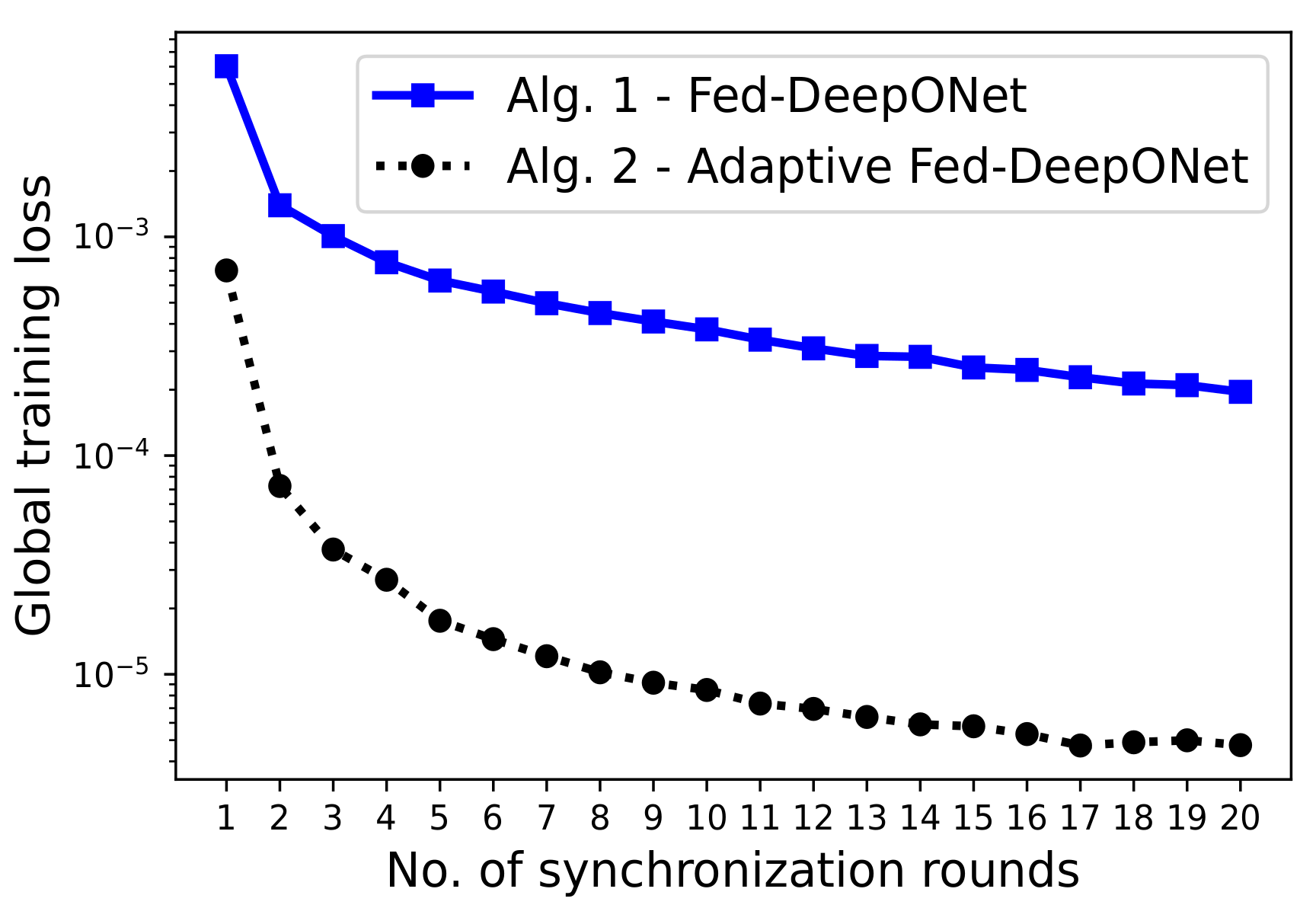
In our first experiment, we quickly verify our previous statement that Algorithm 1 presents slow convergence when training Fed-DeepONets. To this end, we construct an idealized federated training scenario and compare the global training convergences of Fed-DeepONet (Algorithm 1) and Adaptive Fed-DeepONet (Algorithm 2). The proposed idealized scenario assumes we have $C=20$ clients and a fraction $\alpha =0.75$ of the C clients, selected uniformly at random at each global synchronization round, perform federated training. The federated dynamics are controlled by the number of synchronization rounds and the number of local updates, which we set, respectively, to the values $R=20$ and $K=200$.

Figure 2 depicts the results of applying federated training using Algorithm 1 and Algorithm 2. Notice that, as expected, the training convergence of Fed-DeepONet is poor compared to the training convergence of the Adaptive Fed-DeepONet. We remark that this result is not new. In centralized deep learning [27], even though most of the theoretical results are developed for stochastic gradient descent (SGD), one often uses adaptive versions of SGD in practice. These adaptive methods generally deal better with the non-convex nature of the loss function and training dynamics. These results motivate us to only employ the Adaptive Fed-DeepONet to demonstrate the proposed framework’s performance.

4.2. Experiment 2: Learning the Pendulum’s Solution Operator G

In this experiment, we used the adaptive Fed-DeepONet to approximate the solution operator G of the gravity pendulum with control input u described above.

Verifying the performance of Fed-DeepONet. In this experiment, we tested the proposed Fed-DeepONet using $C=20$ as the available clients. Notice that the number of clients C is a problem-dependent parameter. However, since we are interested in learning solution operators of complex dynamical systems, the potential applications for Fed-DeepONet may have a small number of clients. This motivates us to consider cases where the number of clients satisfies $C\le 50$. Further, we set the number of global synchronization DeepONet rounds to $R=20$ and the number of local updates to $K=200$ using a simple routine of hyper-parameter optimization [27]. We remark, however, that, in practice, one may need to select the parameter values for K and R considering problem-dependent constraints, such as computational resources, communication resources, near real-time performance, or cyber-security.

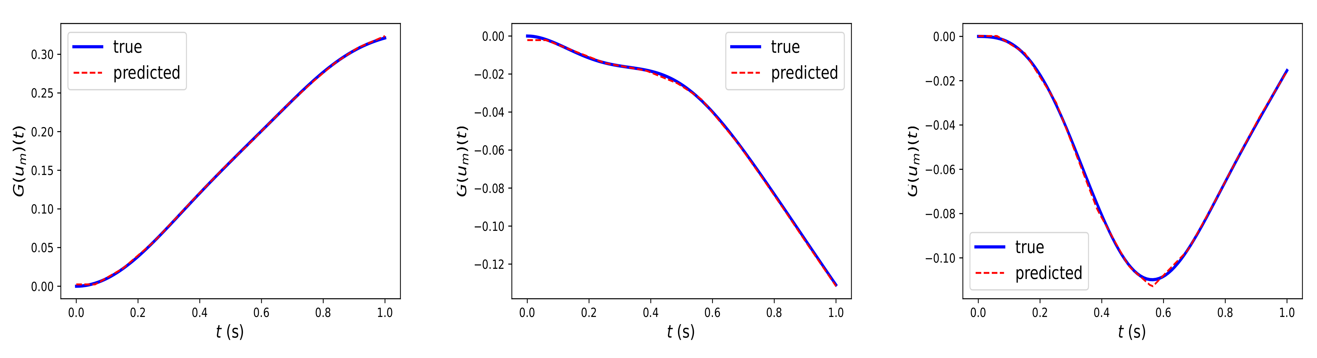
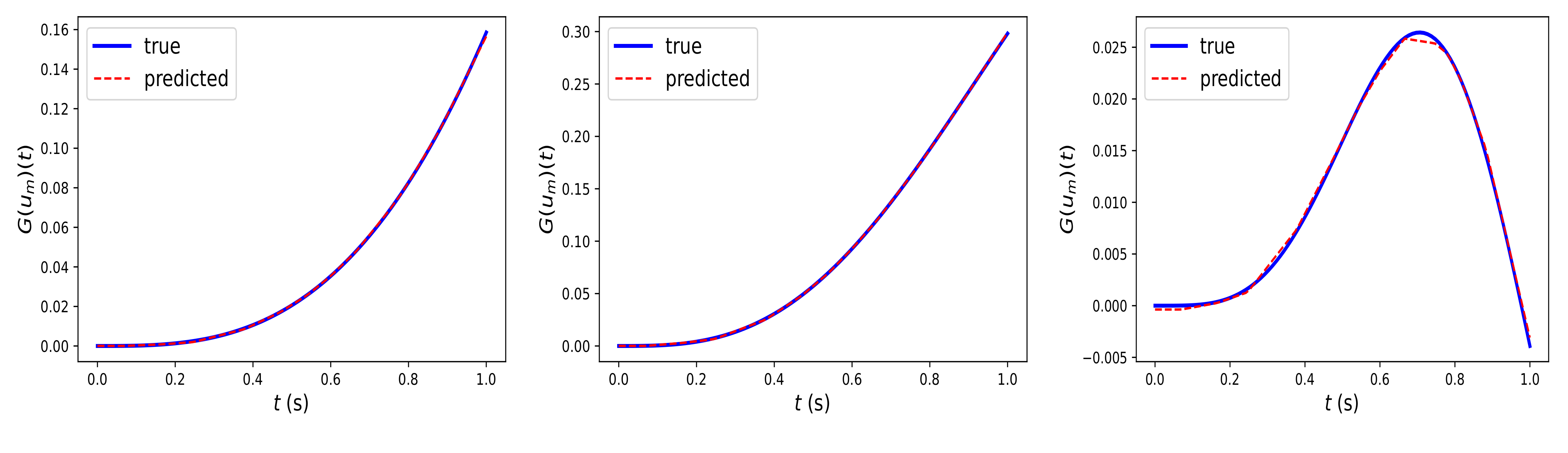
Figure 3 illustrates the prediction of the trained Fed-DeepONet $G_{{\theta }^{*}}$ via Algorithm 2 for three solution trajectories driven by test input trajectories generated using the GRF and not included in the training dataset. Furthermore, we computed the mean $L_2$-relative error using the 100 test trajectories. We obtained a mean $L_2$-relative error of $e_{L2}=1.362$%. Such a result illustrates the potential of DeepONet for protecting clients’ data privacy or employing high-performance distributed computing frameworks while preserving the extraordinary prediction capability of the centralized DeepONet.

Similarly, Figure 4 depicts the prediction of Fed-DeepONet $G_{{\theta }^{*}}$, trained using Algorithm 2, for the solution trajectories driven by the out-of-distribution inputs $u\left(t\right)\in \{t,sin(\pi t),tsin(2\pi t\left)\right\}$. The results illustrate that Fed-DeepONet preserves the generalization capability of the centralized DeepONet.

Testing the sensitivity of Fed-DeepONet with respect to design parameters. This experiment tests the sensitivity of FeedDeepONet against the number of clients C and the fraction of available clients, which we denote as $\alpha \in (0,1]$. First, we fixed the fraction of available clients to $\alpha =0.75$ and varied the number of clients within set $C\in \{10,20,40,50\}$. Then, we fixed the number of clients to $C=20$ and varied the fraction of available clients within the set $\alpha \in \{0.25,0.5,0.75,1.0\}$.

Table 1. The mean and standard deviation of the $L_2$-relative errors computed when predicting with Fed-DeepONet $G_{{\theta }^{*}}$ 100 test solution trajectories driven by control inputs generated from a Gaussian Random Field and a variable number of clients within the set $C\in \{10,20,40,50\}$.

# of Clients C	10	20	40	50
mean $e_{L_2}$	0.989%	1.154%	1.815%	2.613%
st.dev. $e_{L_2}$	1.069%	1.543%	2.057%	4.043%

and

Table 2. The mean and standard deviation of the $L_2$-relative errors computed when predicting with Fed-DeepONet $G_{{\theta }^{*}}$ 100 test solution trajectories driven by control inputs generated from a Gaussian Random Field and variable fraction of available clients within the set $\alpha \in \{0.25,0.5,0.75,1.0\}$.

Frac. Available Clients $\mathit{\alpha }$	0.25	0.5	0.75	1.0
mean $e_{L_2}$	1.495%	1.324%	1.154%	1.362%
st.dev. $e_{L_2}$	1.362%	2.091%	1.543%	1.316%

depict the mean and standard deviation of the $L_2$-relative errors $e_{L_2}$ for the solution trajectories obtained using the 100 test input trajectories for different numbers of clients C or fractions of available clients $\alpha$. The results illustrate that Fed-DeepONet is robust to the different possible configurations of federated training.

Enabling different fractions of available clients during federated training. In this experiment, we tested the performance of the Adaptive Fed-DeepONet using a more realistic scenario, where fraction $\alpha$ of available clients is time-dependent, i.e., it can vary during federated training. To this end, we fix the number of clients to $C=20$ and allow the fraction of available clients to vary at each global synchronization round. In particular, we let $\alpha$ take any value within the interval $[0.1,1.0]$. In other words, we always have at least 10% of clients available for federated training. After employing Fed-DeepONet, the mean and standard deviation of the $L_2$-relative errors $e_{L_2}$ for the solution trajectories obtained using the 100 test input trajectories are, respectively, $1.016$% and $0.845$%. Clearly, these results illustrate that even in this more realistic scenario, the adaptive Fed-DeepONet framework can effectively learn such a complex infinite dimensional operator.

4.3. Experiment 3: Fed-DeepONet and Data Heterogeneity

To test the effect of data heterogeneity on the performance of Fed-DeepONet Algorithms 1 and 2, we designed the following two experiments.

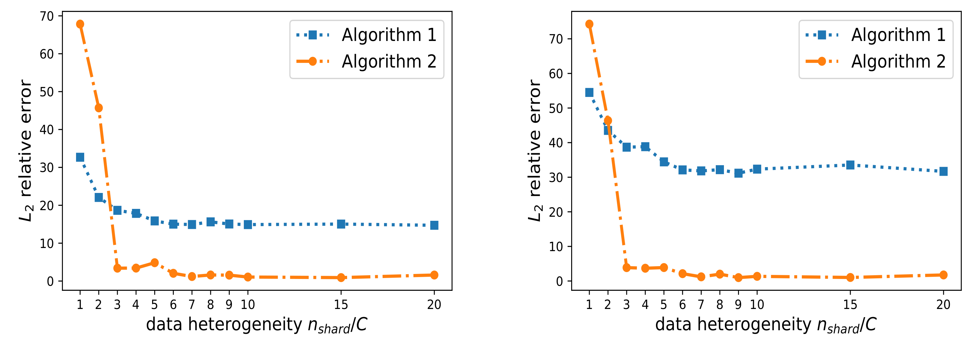
In the first experiment, we modify the amount of data heterogeneity as follows. Consider the centralized dataset ${\mathcal{D}}_{\mathrm{cent}}$ with N data triplets $\{u_m^{\left(k\right)},y^{\left(k\right)},G\left(u_m^{\left(k\right)}\right)\left(y^{\left(k\right)}\right)\}$. We sort this dataset according to the target operator values $G\left(u_m^{\left(k\right)}\right)\left(y^{\left(k\right)}\right)$ (i.e., from smallest to largest). Then, we divide the sorted dataset into $n_{\mathrm{shards}}$ blocks/shards (for simplicity, we let $n_{\mathrm{shard}}\ge C$). We then assign to each of the clients $n_{\mathrm{shards}}/C$ blocks for sampling data. Notice that as the value of $n_{\mathrm{shards}}/C$ increases, the federated dataset becomes more independent and identically distributed. This is because the clients can get data from multiple blocks, making the data samples more diversified. As a result, the densities $p_i(\{u_m,y\},G\left(u_m\right)\left(y\right))$ and $p_j(\{u_m,y\},G\left(u_m\right)\left(y\right))$ become more statistically alike. On the other hand, as the value of $n_{\mathrm{shards}}/C$ decreases, the data heterogeneity increases. In particular, for this simple experiment, the data heterogeneity reaches its maximum when $n_{\mathrm{shards}}=C$.

To verify the effect of data heterogeneity, we consider a federated training scenario with $C=20$ clients and allow the fraction of available clients to vary at each global round. Moreover, we use $R=20$ global synchronization rounds and $K=200$ local updates. Figure 5 (left) (resp. Figure 5 (right)) depicts the mean $L_2$ relative error for 100 in-distribution (resp. out-of-distribution) trajectories when we vary the data heterogeneity (i.e., $n_{\mathrm{shards}}/C\in \{1,2,\dots ,10,15,20\}$). The results show that for the most extreme data heterogeneous setting, i.e., when $n_{\mathrm{shards}}=C$, Algorithm 1 outperforms Algorithm 2. However, in the less extreme data heterogeneity scenarios, Algorithm 2 has an excellent performance, similar to the case when the data collected by each client is independent and identically distributed.

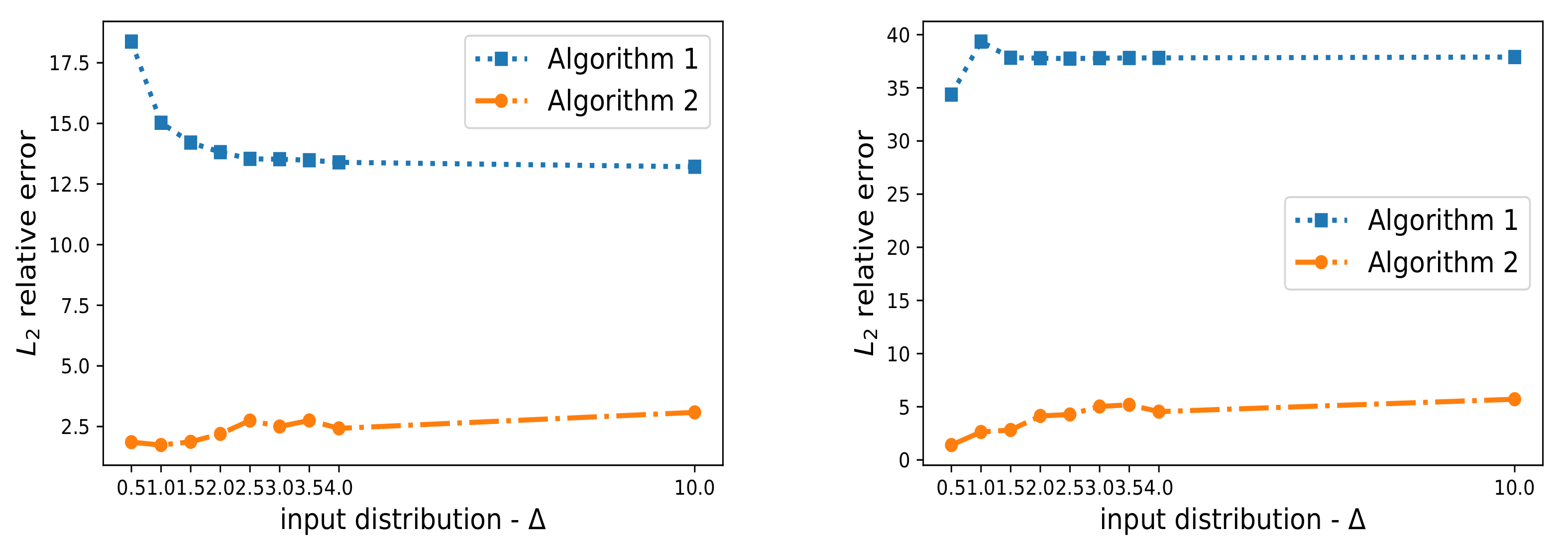
In our second experiment, we modify the input functional distribution (that is, the input data heterogeneity) for some of the C clients. In particular, we use two distinct Gaussian Random Fields (GRF). The first GRF uses the length-scale ${\ell }_1=0.2$ and the second GRF uses ${\ell }_2={\ell }_1+\Delta$. We use the control parameter $\Delta$ to increase the heterogeneity between the two input distributions. We follow a federated training scenario similar to the one described in the previous example and randomly assign one of the input distributions to each of the C clients.

Figure 6 (left) (resp. Figure 6 (right)) depicts the mean $L_2$ relative error for 100 in-distribution (resp. the out-of-distribution) trajectories when we vary the functional input data heterogeneity (i.e., we increase $\Delta$). The results illustrate that as we increase the input data heterogeneity (i.e., as we increase $\Delta \in \{0.5,1.0,1.5,2.0,2.5,3.0,3.5,4.0\}$), the performance of the proposed adaptive Fed-DeepONet (Algorithm 2) does not deteriorate. Such a result shows that Algorithm 2 is robust against changes in the input distribution. Note also that Algorithm 1 is also not affected by the increase in data heterogeneity. The performance of Algorithm 1, however, is not acceptable.

4.4. Experiment 4: Learning a Library of Pendulums

In this experiment, we verified the capability of Fed-DeepONet $G_{{\theta }^{*}}$ trained using Algorithm 2 for approximating the dynamic response of a library of pendulums. That is, we trained the Fed-DeepONet to approximate the dynamic response of all the pendulums whose parameter k satisfies $k\in [0.5,1.5]$. Note that the true solution operator for the library of pendulums is $G(u_m,k)\left(t\right)$ for $t\in [0,T]$. Thus, the desired DeepONet will have two inputs to the Branch network; that is, $u_m$ and k. For testing purposes, we sampled k uniformly within the interval $[0.5,1.5]$.

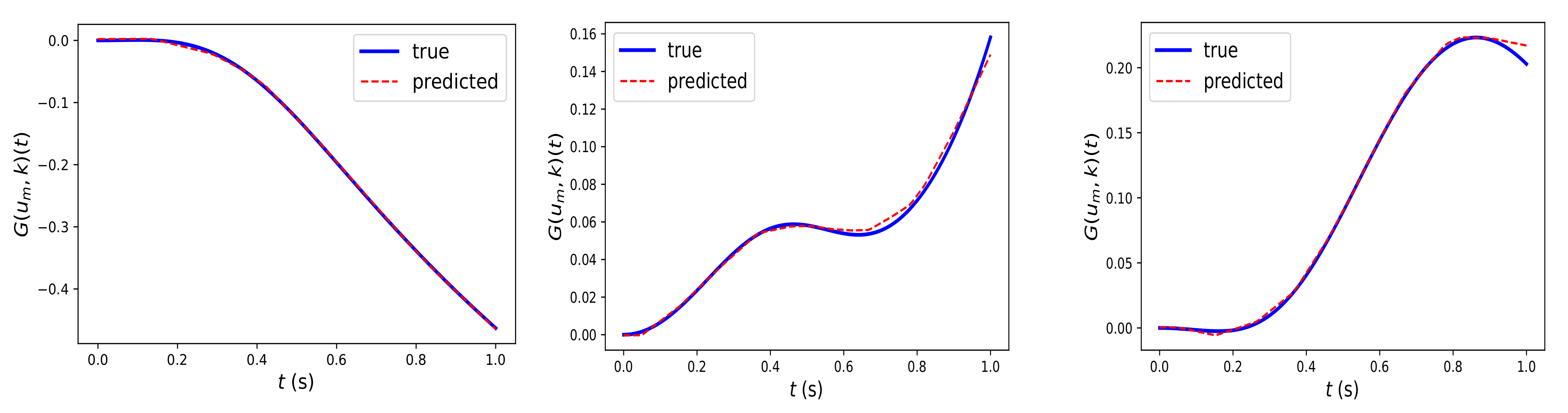
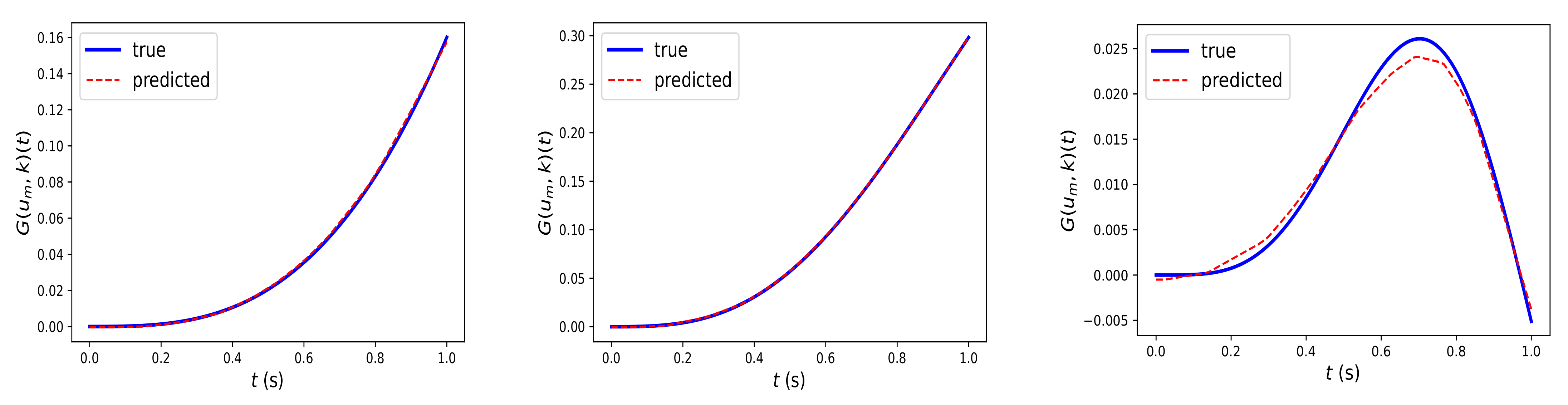
For the experiment, we set $R=20$, $K=200$, $C=50$, and $\alpha =0.5$. Figure 7 (resp. Figure 8) depicts the Fed-DeepONet’s prediction of three solution trajectories driven by three test in-distribution (resp. out-of-distribution) inputs and the parameter k sampled uniformly from the interval $[0.5,1.5]$. Furthermore, the corresponding mean $L_2$-relative error for the 100 (resp. three) solution trajectories driven by the test inputs (resp. the out-of-distribution inputs) is $e_{L_2}=2.582$% (resp. $e_{L_2}=3.347$%). The results clearly show that Fed-DeepONet effectively predicts and generalizes the dynamic response of a parametric library of pendulums.

5. Discussion

Our results: In this paper, we have presented a series of illustrative numerical experiments that aim to provide a glimpse of the potential of Fed-DeepONets for learning the solution operator of complex dynamical systems in a distributed manner. We have shown that the Adaptive Fed-DeepONet is robust to several scenarios, including time-dependent available clients or a different number of clients. We remark, however, that depending on the application, one must carefully select the hyper-parameters used for describing federated learning (e.g., K or R) or the dynamical system under study. For instance, one may obtain the parameter values for Fed-DeepONets using a hyper-parameter optimization routine that respects the underlying constraints of the problem.

The limitations of Fed-DeepONet: The proposed Fed-DeepONet framework has the following limitations. (i) Fed-DeepONet cannot assimilate data in real time. In other words, the federated training of DeepONets must be performed offline. This limitation is a direct consequence of using batch stochastic gradient descent and its variants for neural network training. One may use a distributed version of Kalman Filters to alleviate this limitation. However, training neural network parameters with Kalman Filters is a challenging task. (ii) While Fed-DeepONet protects data privacy, it may not protect the client’s information. A skillful adversary may infer information about the client’s process from observing the parameters transmitted to the central server. A simple solution to alleviate this limitation may be to keep some of the parameters private. (iii) Fed-DeepONet may fail to optimize multi-objective loss functions or constrained problems. This is another limitation inherited from using stochastic gradient descent for unconstrained optimization. Two possible solutions are as follows. One may use a penalty method to transform the problem into an unconstrained one. On the other hand, one may design a federated evolutionary strategy that can handle the underlying multi-objective problem.

Our future work: First, we aim to employ Fed-DeepONet to build digital twins for (i) distributed renewable energy resources and (ii) city-wide predictive models for the transmission of contagious diseases (e.g., COVID-19). Then, we will apply Fed-DeepONet to accelerate material science by enabling training with high-performance distributed and parallel computing platforms. Finally, we aim to extend our federated optimization strategy to a federated sampling strategy that enables quantifying uncertainty for DeepONets.

6. Conclusions

This paper proposed a federated learning strategy for Deep Operator Networks (Fed-DeepONet). In particular, we introduced two algorithms that enabled extending the classical stochastic gradient descent and its momentum-enhanced (i.e., adaptive) version to the federated setting for training DeepONets. As a proof of concept, we illustrated the performance and efficacy of Fed-DeepONet using two experiments. In particular, we trained Fed-DeepONets to allow a collection of clients (not all the clients available all the time) to learn, in a distributed manner, (i) the solution operator of a gravity pendulum and (ii) the dynamic response of a library of pendulums.