Abstract
This paper discusses a method for taking into account rounding errors when constructing a stopping criterion for the iterative process in gradient minimization methods. The main aim of this work was to develop methods for improving the quality of the solutions for real applied minimization problems, which require significant amounts of calculations and, as a result, can be sensitive to the accumulation of rounding errors. However, this paper demonstrates that the developed approach can also be useful in solving computationally small problems. The main ideas of this work are demonstrated using one of the possible implementations of the conjugate gradient method for solving an overdetermined system of linear algebraic equations with a dense matrix.
Keywords:
gradient method; conjugate gradient method; round-off error; rounding error; stopping criteria MSC:
65F10; 65F20; 65F30
1. Introduction
When solving applied inverse problems or optimization problems, it often becomes necessary to minimize some target functionals. Iterative methods are usually used for minimization. If the problem is linear, then one of the most common minimization methods employed is the conjugate gradient method [1]. If the number of components in the required element realizing the minimum of the functional is N, then the conjugate gradient method converges to the exact solution of the problem in exactly N iterations. However, this statement is only true on the condition that all calculations are performed accurately and that there are no rounding errors. Nevertheless, when solving real applied problems, rounding errors can greatly affect the resulting approximate solution. Two cases are possible: In the first case, the value of the minimized functional becomes comparable to the background of rounding errors at some iteration, the number of which is less than N. Starting from this iteration, the value of the functional stops decreasing. This means that starting from this iteration, all subsequent calculations will not improve the solution and are meaningless. Therefore, a reasonable question arises—is it possible to track this moment in order to save computing resources? A positive answer to this question is useful, but not critical in solving real applied problems. On the other hand, the second case is essential for practice. In the second case, due to rounding errors in determining the minimization directions and the steps along them, it turns out that after performing N iterations, the value of the minimized functional is still quite large. This means that the found approximate solution can still be refined if the iterative process is continued. It turns out that the continuation of the iterative process will allow us to find a better approximation for the true solution. We emphasize that here, in contrast to the first case, the classical criterion for stopping the iterative process (by a fixed number of iterations equal to N) gives a bad result. When solving many real applied inverse problems (both 2D and 3D), the authors of this paper regularly encountered a similar problem. To solve this problem, it was necessary to use purely empirical approaches and determine the optimal number of iterations experimentally. However, when solving “large” real problems, this approach required large computational resources. As a result, there was a need to develop a method for automatically determining the number of iterations, in which the value of the minimized functional becomes comparable to the background of rounding errors. Therefore, taking into account rounding errors when choosing a criterion to stop the iterative process is a relevant issue and in demand in practice.
A thorough study of this issue showed that there are practically no research works on this topic. Most of the works that contain recommendations concerning the choice of the stopping criterion of the iterative process in gradient methods do not take into account rounding errors (for example, see [2,3,4,5,6,7,8,9,10,11,12,13,14,15,16,17,18,19,20,21]). The authors are only aware of one study dedicated to this subject: the work by Kalitkin et al. in [22]. However, the derivation of the corresponding formulas in this work contains many unfounded assumptions. This was the authors’ motivation for constructing their own version of these formulas. In this work, we would like to demonstrate the methodology for deriving the corresponding formulas; we intend to show this through the application of the conjugate gradient method to solve an overdetermined system of linear algebraic equations with a dense matrix. If desired, similar formulas for solving nonlinear systems can be constructed. In this case, one cannot be limited to the conjugate gradient method but must be able to use any gradient method, for which its own criterion to stop the iterative process upon entering the background of rounding errors will be obtained. The choice of the conjugate gradient method as an example is justified by the fact that for this method, there is a classical criterion for stopping the iterative process with which we can compare our approach.
Separately, we would like to draw attention to how accounting for rounding errors is, in our opinion, especially relevant now, when supercomputer systems are available to many researchers for the calculation of real “large” problems. This is due to the fact that the use of high-performance computing systems makes it possible to carry out huge amounts of calculations. However, the more calculations we perform, the more rounding errors can accumulate over the course of a computation. The more errors are accumulated, the more unreliable the results can be if we apply the criteria to stop the iterative process, which do not take this error into account. However, despite this, we will demonstrate in this paper that these formulas can give good results even in the case of solving “small” problems.
The structure of this work is as follows. Section 2 contains the statement of the problem and the formula of one of the possible implementations of the conjugate gradient method to obtain its solution. Section 3 demonstrates the derivation of formulas for the stopping criterion of the iterative process, which takes into account the rounding errors. Section 4 discusses the computational complexity of the proposed algorithm. Section 5 formulates a version of the conjugate gradient method that we are considering, with an improved stopping criterion of the iterative process. Section 6 contains examples of calculations demonstrating the effectiveness of the proposed approach.
2. Problem Statement
Consider one of the possible implementations of the conjugate gradient method for solving an overdetermined system of linear algebraic equations with a dense matrix:
Here, A is a rectangular matrix of dimension (), and b is a column vector with M components. It is necessary to find x, which is a column vector with N components.
When solving real applied problems, the components of the vector b are usually measured experimentally. Therefore, due to the presence of experimental errors, this system may not have a classical solution. However, with a sufficient number of input data ( and the data do not duplicate each other), it is possible to find a pseudo-solution to this problem using the least squares method:
Here, and below , is the Euclidean norm.
Remark 1.
It is well-known that many real applied problems are ill-posed [23]. When solving them, it is necessary to construct regularizing algorithms. Most often, these algorithms are based on the minimization of some modified functionals. An example of such a functional is the functional of A. N. Tikhonov [23]: (here, α is the regularization parameter, and the matrix R defines a priori constraints). In this paper, to simplify the presentation, we will assume that the problem under consideration is well-posed. However, the formulas obtained below can be easily generalized to the mentioned case.
There are many ways to find the vector x. We have chosen the one that is the most indicative within the framework of this work.
Hence, the vector x with N components, which is a solution (pseudo-solution) of system (1), can be found using the following iterative algorithm, which constructs the sequence . This sequence converges in N steps to the desired solution (pseudo-solution) of system (1), based on the assumption that all calculations are performed exactly.
We set , , and an arbitrary initial approximation . Then, we repeatedly perform the following sequence of actions:
We emphasize that in this case, the classical criterion for stopping the iterative process is formulated as follows: calculations are carried out while .
As a result, after N steps, the vector will be regarded as a solution (pseudo-solution) of system (1).
Remark 2.
If we do not use the recurrent notation and calculate the residual in each iteration in the same way as in the first iteration, then the number of arithmetic operations required to complete the iterative process will double. This is the motivation for using the recurrent form of the conjugate gradient method when solving “large” problems.
Formally, this algorithm with the classical stopping criterion of the iterative process is formulated as follows:
- Set , , and an arbitrary initial approximation .
- Compute and go to step 4.
- Compute .
- Compute .
- Compute .
- Compute .
- If , then stop the iterative process and set as a solution of system (1).
- Redefine and go to step 3.
3. Improved Criterion for Stopping the Iterative Process
We will stop the iterative process at the iteration when the norm of the residual ceases to exceed the rounding errors that occur during its calculation. In other words, it makes sense to continue the iterative process as long as the following inequality remains true:
Here, is the variance of the error of the residual norm at the s-th iteration in units of , with being the relative rounding error. In calculations with double precision, (float64) ; in calculations with quad precision, (float128) . Next, we describe a method for estimating the value of .
Let us start by estimating the error of each of the elements of the vector in the first iteration :
We will estimate errors from addition according to the rules of statistics, i.e., . Errors from multiplication are quite small compared to errors from addition, so we will not take them into account.
Then,
With the subsequent multiplication, the resulting error variances also increase by the corresponding factor squared:
Finally, summing over k, we get the formula below:
Next, we will consider the calculation of the error for the components of the vector in iterations . In these iterations, we rewrite the recurrent formula for calculating the residual in the following form:
The error variance can be calculated using partial derivatives with respect to the independent components. However, taking into account all possible values in previous iterations will lead to an overestimation of the error. To avoid this, we take into account the peculiarity of gradient methods, which consists of the fact that gradient methods are resistant to some parts of rounding errors because in each iteration, some of the errors are compensated. This is due to the fact that each iteration of the gradient method can be interpreted as a way to find the next better approximation of the desired solution based on a previous iteration.
The first way to calculate . We will assume that when calculating the vector , it does not make sense to take into account all previous errors (because is the direction of minimization). Thus, only rounding errors which arise when using the value of in further calculations remain. Taking this into account, we get the following equations:
Here, the expressions for the error variances of the calculation of the vector components are calculated using already known formulas, such as:
The second way to calculate . To significantly simplify (in terms of the number of operations) the calculation of error variances in each iteration of the gradient method, we can assume that it is not necessary to take into account all previous errors, not only when calculating the vector , but also when calculating the vector . Taking this into account, we get the following equation:
After calculating with any of the methods, the error variance of the residual norm is calculated as the sum of the variances of the components since they are independent of each other, which is expressed as follows:
When the condition
is met, the iterative process is interrupted, and the vector is chosen as a solution of the system (1).
This is the improved criterion for stopping the iterative process.
4. On Increasing Computational Complexity
Note that in the gradient method under consideration, starting from , the most computationally intensive operation in each iteration is the operation that calculates . It requires arithmetic operations to compute the vector and arithmetic operations to compute the final value . That is, the total number of arithmetic operations for computing is . The remaining operations in each iteration of the gradient method make a much smaller contribution to the total number of arithmetic operations, so we estimate the computational complexity of each iteration of the gradient method as .
Once again, we also emphasize the advantage of the recurrent calculation of the residual in all iterations, starting from . If we do not use the recurrent notation and then calculate the residual in each iteration in the same way as in the first iteration, then the number of arithmetic operations required to complete the iterative process will increase by about two times.
An important question arises: does the computational complexity of the algorithm increase when using the new stopping criterion?
The first way to calculate requires about additional arithmetic operations in each iteration of the considered gradient method. One can accurately calculate all arithmetic operations; in order to achieve this, one needs to consider the most computationally intense part—the calculation components of . This operation requires arithmetic operations to compute the elements of the inner sum, and then more arithmetic operations to compute the outer sum. In total, operations are obtained, which increases the computational complexity of the considered gradient method by about 2.5 times.
The second way to calculate requires only about additional arithmetic operations. This means that the computational complexity of the considered gradient method will not change in order.
The use of both approaches in solving a large number of applied problems has shown that both methods give approximately the same results. In this regard, in the test calculations in Section 6, we will use only the second method as it is the most economical in the computational sense. However, we will first formulate this version of the conjugate gradient method with an improved stopping criterion of the iterative process.
5. Improved Iterative Algorithm
Thus, the iterative algorithm for solving system (1) with an improved stopping criterion of the iterative process will take the following form:
- Set , and an arbitrary initial approximation .
- Compute .
- Compute for each and go to step 6.
- Compute .
- Compute for each .
- Compute .
- If , then stop the iterative process and set as a solution of system (1).
- Compute .
- Compute .
- Compute .
- Redefine and go to step 4.
6. Examples of Numerical Experiments
To demonstrate the capabilities of the proposed algorithm, we denote the following: (1) a matrix A of dimension , with elements generated as random variables with a uniform distribution in the range ; (2) a model solution —a column vector of dimension N whose elements correspond to the values of the sine on the interval .
For the matrix A and the model solution , the right side b was calculated as follows: . To solve system (1) with this matrix and the right side, the considered variation of the conjugate gradient method with an improved criterion for stopping the iterative process was used. All calculations were performed in double precision (float64), i.e., .
Remark 3.
Note that all subsequent results may slightly differ in details when reproduced since the matrix A is given randomly.
Example 1.
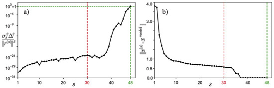
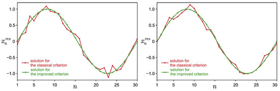
Calculations were made for and . These parameters were especially selected to better demonstrate the capabilities of the algorithm under consideration. Figure 1a shows a graph of depending on the iteration number s. The classical stopping criterion for the iterative process would have stopped at the iteration with the number (marked in the figure with the red dotted vertical line), but the improved criterion stopped the iterative process only at the iteration with the number , i.e., much later. Figure 1b shows the dependence of on the iteration number s. It is clearly seen from the graph that the classical criterion for stopping the iterative process gives a solution that is quite different from that of the model. Now, let us see what the approximate solutions look like in the case of using different criteria to stop the iterative process. Figure 2 shows an approximate solution—vector . It is perfectly clear that the approximate solution found by the classical method (marked in red on the graph) is quite different from the exact one (sine), even visually. In this case, the solution found using the improved criterion for stopping the iterative process no longer visually differs from the exact solution. That is, we managed to demonstrate the efficiency of the proposed algorithm with the use of such a simple example, although it was initially assumed that the method would work only when solving “large” problems.
Figure 1.
Example 1: (a) Graph of depending on the iteration number s. (b) Graph of depending on the iteration number s.
Figure 2.
Example 1: Graph of depending on the component index n. Figures correspond to two different arbitrary matrices A.
Example 2.
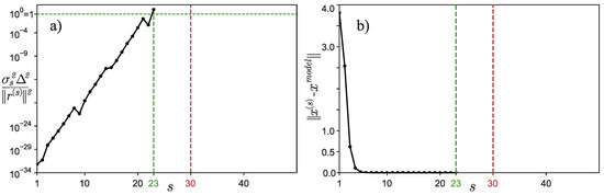
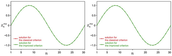
Let us now carry out a numerical experiment for and . It can be seen from Figure 3a that the classical stopping criterion for the iterative process would have worked at iteration number , but the improved criterion stopped the iterative process much earlier, namely at iteration . Figure 3b confirms that the classical criterion for stopping the iterative process was triggered too late, and many iterations were wasted. Moreover, the approximate solution found by the classical method is indistinguishable from the solution found using the improved criterion for stopping the iterative process—the graphs overlap and are visually indistinguishable from each other (see Figure 4), which is the rationale for the early termination of the iterative process.
Figure 3.
Example 2: (a) Graph of depending on the iteration number s. (b) Graph of depending on the iteration number s.
Figure 4.
Example 2: Graph of depending on the component index n. Figures correspond to two different arbitrary matrices A. Solutions for different criteria for stopping iterative processes are visually indistinguishable from each other (graphs overlap).
7. Discussion
- Algorithms equivalent to those proposed in this paper can be derived in a sufficiently large number of ways. It is quite possible that some versions of the proposed algorithm will work better for some specific applied problems, but worse for others. However, at the same time, it is important that the proposed variants of the formulas do not greatly increase the computational complexity of the algorithm.
- Many systems of algebraic equations (both linear and non-linear) arise when solving ill-posed problems [23]. In this case, regularizing algorithms are constructed; in the application of these algorithms, one of the key points is the question of a reasonable choice for the regularization parameter. In this regard, the question remains as to how the rounding error could be correctly taken into account when automatically choosing the regularization parameter in accordance with the input data specification errors (for example, see the generalized residual principle in [23]).
- The method considered in this paper assumes that the measure of inconsistency of the solved system of equations is sufficiently small. When solving problems with a sufficiently large measure of inconsistency, one should additionally monitor the iteration of the algorithm when the value of the discrepancy ceases to decrease. In this case, the iterative process must be interrupted without waiting for the value of the functional to enter the background of the rounding errors.
- The formulas presented in this paper were derived from statistical considerations. Therefore, the reliability of the proposed algorithm is quite high when solving “large” problems with high-precision computation. However, there are practical problems in which calculations with low-precision computation are actively used. For example, in current machine learning implementations, low-precision computation, e.g., half-precision (float16, ), is used to alleviate the burden on the limited CUDA memory. The results of applying the algorithm proposed by the authors for calculations with such low precision may have the following features: On the one hand, situations are still possible in which the algorithm proposed by the authors will give a good result. For example, in Figure 5, the results of such calculations for and () are presented. On the other hand, the low-precision computation leads to the rounding error becoming comparable to the residual quite early. As a result, this may lead to the iterative process stopping earlier than necessary. For example, in Figure 6, the results of such calculations for and () are presented. The non-fulfillment of statistical considerations is perfectly confirmed by the non-monotonicity of the curve of depending on the iteration number s (see Figure 6b). However, taking into account the fact that calculations with low precision are used in applications where higher precision is not essential, the result shown in Figure 6a can be quite adequate and meet practical needs. At the same time, we note that no solution was found by the classical algorithm (there is no corresponding curve in Figure 6b), which is due to the fact that the effect of numerical overflow had emerged. The use of the improved criterion made it possible to avoid this effect due to the early termination of the iterative process.
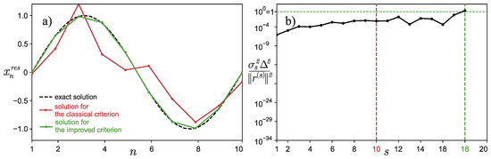 Figure 5. (a) Graph of depending on the component index n. (b) Graph of depending on the iteration number s.
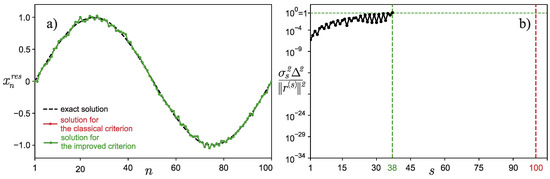 Figure 6. (a) Graph of depending on the component index n. (b) Graph of depending on the iteration number s.
8. Conclusions
This paper considered a method for taking into account rounding errors when constructing the criteria to stop the iterative process in gradient minimization methods. This method was originally developed by the authors to solve computationally intensive applied problems. However, numerous numerical experiments have shown (much to the surprise of the authors) that the considered method also works when solving computationally small problems, during which the occurrence of the corresponding problems is not at all obvious.
Author Contributions
Conceptualization, D.L.; methodology, D.L., V.S. and A.Y.; software, D.L. and V.S.; validation, D.L. and V.S.; formal analysis, D.L. and V.S.; investigation, D.L. and V.S.; resources, D.L. and V.S.; data curation, D.L. and V.S.; writing—original draft preparation, D.L.; writing—review and editing, D.L.; visualization, D.L. and V.S.; supervision, D.L.; project administration, A.Y.; funding acquisition, D.L. and A.Y. All authors have read and agreed to the published version of the manuscript.
Funding
This paper was published with financial support from the Ministry of Education and Science of the Russian Federation as part of the program of the Moscow Center for Fundamental and Applied Mathematics under the agreement N 075-15-2019-1621.
Data Availability Statement
Not applicable.
Conflicts of Interest
The authors declare no conflict of interest.
References
- Hestenes, M.; Stiefel, E. Methods of conjugate gradients for solving linear systems. J. Res. Natl. Bur. Stand. 1952, 49, 409. [Google Scholar] [CrossRef]
- Bottou, L.; Curtis, F.E.; Nocedal, J. Optimization methods for large-scale machine learning. SIAM Rev. 2018, 60, 223–311. [Google Scholar] [CrossRef]
- Patel, V. Stopping criteria for, and strong convergence of, stochastic gradient descent on Bottou-Curtis-Nocedal functions. Math. Program. 2021, 1–42. [Google Scholar] [CrossRef]
- Callaghan, M.; Müller-Hansen, F. Statistical stopping criteria for automated screening in systematic reviews. Syst. Rev. 2020, 9, 273. [Google Scholar] [CrossRef] [PubMed]
- Nikolajsen, J. New stopping criteria for iterative root finding. R. Soc. Open Sci. 2014, 1, 140206. [Google Scholar] [CrossRef] [PubMed]
- Polyak, B.; Kuruzov, I.; Stonyakin, F. Stopping rules for gradient methods for non-convex problems with additive noise in gradient. arXiv 2022, arXiv:2205.07544. [Google Scholar]
- Kabanikhin, S. Inverse and Ill-Posed Problems: Theory and Applications; Walter de Gruyter: Berlin, Germany, 2011. [Google Scholar]
- Vasin, A.; Gasnikov, A.; Dvurechensky, P.; Spokoiny, V. Accelerated gradient methods with absolute and relative noise in the gradient. arXiv 2022, arXiv:2102.02921. [Google Scholar]
- Cohen, M.; Diakonikolas, J.; Orecchia, L. On acceleration with noise-corrupted gradients. In Proceedings of the 35th International Conference on Machine Learning, 2018, Stockholmsmässan, Sweden, 9 February 2018. [Google Scholar]
- Dvurechensky, P.; Gasnikov, A. Stochastic intermediate gradient method for convex problems with stochastic inexact oracle. J. Optim. Theory Appl. 2016, 171, 121–145. [Google Scholar] [CrossRef]
- Gasnikov, A.; Kabanikhin, S.; Mohammed, A.; Shishlenin, M. Convex optimization in Hilbert space with applications to inverse problems. arXiv 2017, arXiv:1703.00267. [Google Scholar]
- Rao, K.; Malan, P.; Perot, J.B. A stopping criterion for the iterative solution of partial differential equations. J. Comput. Phys. 2018, 352, 265–284. [Google Scholar] [CrossRef]
- Arioli, M.; Duff, I.; Ruiz, D. Stopping Criteria for Iterative Solvers. SIAM J. Matrix Anal. Appl. 1992, 13, 138–144. [Google Scholar] [CrossRef]
- Arioli, M.; Noulard, E.; Russo, A. Stopping criteria for iterative methods: Applications to PDE’s. Calcolo 2001, 38, 97–112. [Google Scholar] [CrossRef]
- Arioli, M. A stopping criterion for the conjugate gradient algorithm in a finite element method framework. Numer. Math. 2004, 97, 1–24. [Google Scholar] [CrossRef] [Green Version]
- Arioli, M.; Loghin, D.; Wathen, A. Stopping criteria for iterations in finite element methods. Numer. Math. 2005, 99, 381–410. [Google Scholar] [CrossRef]
- Chang, X.W.; Paige, C.C.; Titley-Peloquin, D. Stopping Criteria for the Iterative Solution of Linear Least Squares Problems. SIAM J. Matrix Anal. Appl. 2009, 31, 831–852. [Google Scholar] [CrossRef]
- Axelsson, O.; Kaporin, I. Error norm estimation and stopping criteria in preconditioned conjugate gradient iterations. Numer. Linear Algebra Appl. 2001, 8, 265–286. [Google Scholar] [CrossRef]
- Kaasschieter, E.F. A practical termination criterion for the conjugate gradient method. BIT Numer. Math. 1988, 28, 308–322. [Google Scholar] [CrossRef]
- Jiránek, P.; Strakoš, Z.; Vohralík, M. A posteriori error estimates including algebraic error and stopping criteria for iterative solvers. SIAM J. Sci. Comput. 2010, 32, 1567–1590. [Google Scholar] [CrossRef]
- Landi, G.; Loli Piccolomini, E.; Tomba, I. A stopping criterion for iterative regularization methods. Appl. Numer. Math. 2016, 106, 53–68. [Google Scholar] [CrossRef]
- Kalitkin, N.; Kuz’mina, L. Improved forms of iterative methods for systems of linear algebraic equations. Dokl. Math. 2013, 88, 489–494. [Google Scholar] [CrossRef]
- Tikhonov, A.; Goncharsky, A.; Stepanov, V.; Yagola, A. Numerical Methods for the Solution of Ill-Posed Problems; Kluwer Academic Publishers: Dordrecht, The Netherlands, 1995. [Google Scholar]
Publisher’s Note: MDPI stays neutral with regard to jurisdictional claims in published maps and institutional affiliations. |
© 2022 by the authors. Licensee MDPI, Basel, Switzerland. This article is an open access article distributed under the terms and conditions of the Creative Commons Attribution (CC BY) license (https://creativecommons.org/licenses/by/4.0/).